


Bringing to Light the Potential of Angular Nighttime Composites for Monitoring Human Activities in the Brazilian Legal Amazon

Earth Observation and Geoinformatics Division (DIOTG), National Institute for Space Research (INPE), São José dos Campos 12227-010, Brazil
*
Author to whom correspondence should be addressed.
Remote Sens. 2023, 15(14), 3515; https://doi.org/10.3390/rs15143515
Submission received: 2 February 2023
/
Revised: 25 May 2023
/
Accepted: 5 June 2023
/
Published: 12 July 2023
(This article belongs to the Special Issue Remote Sensing in the Amazon Biome)
Abstract
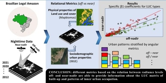
:The Brazilian Legal Amazon (BLA) is the largest administrative unit in Brazil. The region has undergone a series of territorial policies that have led to specific conditions of occupation of the land and particular urban environments. This plurality expresses specific physical relations with the environment and infrastructure, which require innovative methods for detecting and profiling human settlements in this region. The aim of this work is to demonstrate how angular composites of nighttime lights can be associated with specific profiles of urban infrastructure, sociodemographic parameters, and mining sites present in the BLA. We make use of sets of yearly VNP46A4 angular composites specifically associated with the narrowest ranges of observations across the year, i.e., observations right below the sensor’s pathway (near-nadir range) and observations in between the oblique range (off-nadir), to identify urban typologies that expose the presence of structures such as vertical buildings, industrial sites, and areas with different income levels. Through a non-parametric evaluation of the simple difference in radiance values ranging from 2012 to 2021, followed by an ordinary least squares regression (OLS), we find that off-nadir values are persistently higher than near-nadir values except in areas where obstructing structures and particular anisotropic characteristics are present, generally changing trends of the so-called angular effect. We advocate that relational metrics can be extracted from the angular annual composites to provide additional information on the current urban structural state. By calculating the simple difference (DIF), the relative difference (REL), and the residual values of the linear regression formula estimated for the off-nadir and near-nadir composites (RES), it is possible to differentiate urban environments by their physical aspects, such as high-mid income areas, low-income settlements with different levels of density, industrial sites, and verticalized areas. Moreover, pixels that were exclusively found in one of the angular composites could be spatially associated with phenomena such as the overglow effect for the exclusive off-nadir samples and with the wetlands of the northwest portion of the Amazon Forest for the near-nadir samples. This work deepens our current understanding of how to optimize the use of the VNP46A4 angular series for monitoring human activities in the Amazon biome and provides further directions on research possibilities concerning nighttime light angular composites.
1. Introduction
Over the last decades, the Brazilian Legal Amazon (BLA) has been the stage for the main economic policies for the occupation of the national territory in Brazil. Added to the agrarian conflicts, the result is a singular and out-of-step process of development if compared to other regions of the country [1,2].
Currently, this singularity is expressed by a diversity of human settlement types. Among these settlements, there are a few distinctive examples that compose the Amazonian environment, such as secular indigenous villages, small rural communities, settlements that emerged from the local demand for labor focused on extractive activities, small urban centers on the riverbanks that developed from intermediate trading posts for the flow of forest products, cities developed from settlement projects driven by the public sector, cities based on the agricultural economy, and large metropolises that received funding for the development of specific economic sectors, among others [3,4,5,6,7,8]. Each of these settlement categories has its own proper spatial arrangement and inter- and intra-specific infrastructural characteristics that are a reflection of their local economy and the development policy to which they were subjected [5,6,9].
From a broader perspective, monitoring the Amazon is a foundation for understanding regional economic dynamics, evaluating the results of social, environmental, and economic policies, and providing accurate information about different aspects of its territory. This understanding and availability of information are central when highlighting local needs, which are usually neglected by traditional development policies [10,11,12,13].
Given the importance of monitoring the Amazon territory and the challenging task of accessing updated and parameterized data about the infrastructure related to human occupation, remote sensing products are currently one of the main tools for acquiring synoptical, precise, and up-to-date information [14]. Therefore, in the geospatial context, developing methodologies and exploring different sensors and data to further understand the components of this region are crucial steps for its management. The remote sensing of nighttime lights has unexplored potential for this task.
One of the main expressions of human settlements and other anthropogenic processes that stands out in the landscape is the night lighting infrastructure, necessary for the maintenance of various activities at night. During the day, the presence of lighting objects is not evident at certain scales, but at night, light emitted by street lights and other outdoor lighting apparatus can be easily identified [15]. For this reason, satellite images obtained during the night have been tested for their potential to locate and characterize anthropogenic structures and activities that may be somehow associated with the distribution, intensity, and other parameters of nighttime stable lights, including in the Amazon biome, e.g., Refs. [16,17,18,19,20,21].
Although the use of nighttime images is not as consolidated as approaches based on daytime images, in the last decade, an increasing number of studies have explored its usefulness in different fields. Identification of maritime vessels, mapping illegal mining activities, mapping human settlements, population volume estimation at different scales, and estimation of road traffic flow [18,19,20,22,23] are just a few of the fields of study that have successfully identified the potential of nighttime images.
Multiple sources have been used to study issues related to this work’s objectives [19,24,25]. Nonetheless, images of the Day Night Band (DNB) sensor on board the Visible Infrared Imaging Radiometer Suite instrument (VIIRS) are one of the main sources of orbital nighttime images that are uploaded regularly and are freely accessible at the moment. The DNB sensor captures images of the Earth’s surface daily, at approximately 1:30 a.m. local time, depending on the mapped region [26]. After the process of transforming digital numbers into physical quantities, namely, nocturnal radiance, the images from the DNB sensor represent the “brightness” level of the most diverse sources of nighttime lights, such as street lighting structures of cities and other anthropogenic features, auroras, biomass burning, gas flares, and marine vessels, among others [16]. Depending on the objective of the study, the images must be submitted to atmospheric correction processes and also to the compensation of the contribution from other components unrelated to the light emitted by the terrestrial surface, such as the lunar irradiance component [27].
NASA’s Black Marble project is currently one of the main scientific endeavors responsible for making these images available at different processing levels, attending to various demands related to the use of nighttime images [28]. Among the available products, the VNP46A4 series is a set of nighttime composites that refer to annual compositions of images submitted to a rigid process of atmospheric correction and produced from samples only considered of good quality, i.e., without the presence of clouds and other less frequent issues that could compromise the quality of the final product [29]. The final result represents a dataset of the average annual radiance level detected by the DNB sensor, discarding areas that may be affected by ephemeral lights and do not express radiance levels above the detection limit estimated for the sensor.
Recently, angular issues related to the acquisition of nighttime data by the DNB sensor have started to draw researchers’ attention. Some studies have identified that, depending on the angle at which the images are acquired, there is a strong tendency for the instrument to record different levels of radiance associated with the same location [30,31,32]. This phenomenon can be associated with the fact that, although the atmospheric and lunar components of irradiance are treated during the process of retrieving the radiance levels of the DNB data, the methodology still does not use techniques for including the interaction of the electromagnetic radiation (EMR) emitted by outdoor lighting sources with the surrounding environment [29].
The process through which changes in radiance levels for a given location can be detected as a function of the observation angle is called the angular effect. This effect might be caused by the anisotropic emission of radiance from different sources, such as traditional lighting poles that emit radiation preferentially downwards or the interaction of the EMR with surfaces that, in turn, have anisotropic characteristics that affect the EMR’s preferential direction of propagation differently, depending on the set-up of irradiation and imaging [29,30,31,32]. In general, recent studies have treated the angular effect as an aspect to be corrected in the images, since it results in variations in radiative levels that do not express actual changes in the emitted radiative levels [31,32].
This work seeks to address the angular effect as a potential source of environmental information related to local infrastructure, since this effect is closely correlated with aspects such as vegetation cover, height and size of buildings, type of lighting, and radiative intensity [31]. All these aspects are important elements that compose the urban and rural landscape and also support the description of anthropogenic processes in the BLA.
The analyses presented in this paper are based on the use of annual compositions to demonstrate the potential and limitations of the angular sets for monitoring the BLA, specifically the VNP46A4 series. First, the simple differences between the compositions referring to observations carried out only at sets of specific angles were addressed.
When close to the nadir, angular compositions are called near-nadir composites (viewing angles just below the satellite’s pathway). When at oblique angles, they are called off-nadir composites [29]. Second, we investigated the relationship between the spatial distribution of pixels in which only one of the angular compositions was able to detect considerable stable radiance levels and different land use and cover (LUC) classes that compose the context of the VIIRS/DNB pixel’s footprint. Finally, the relationship between the radiance levels of the angular compositions was investigated using a linear regression between a set of samples, which resulted in a proposal for the interpretation of their angular coefficients as indicators of the intensity of the angular effect relative to lit areas under different LUC contexts.
This work contributes to the discussion about the main drivers of the angular effect in the use of angular composites of night lights in the Brazilian Legal Amazon territory, indicating the knowledge gaps, potential methods, and limitations regarding the use of annual compositions for BLA monitoring.
2. Materials and Methods
2.1. Database and Basic Processing Procedures
Nighttime annual angular composites (VNP46A4) are made available by NASA’s Black Marble science team at the Level-1 and Atmosphere Archive & Distribution System Distributed Active Archive Center’s website (LAADS—DAAC, ladsweb.modaps.eosdis.nasa.gov, (accessed on 18 June 2022)). The VNP46A4 product represents the average radiance level from daily nighttime retrievals from its DNB sensor. The product is composed of high-quality, cloud-free observations, after atmospheric, terrain, vegetation, snow, lunar, and stray light correction procedures to estimate daily nighttime light levels before averaging. Average radiance values less than 0.5 nW·cm−2·sr−1 are automatically set to zero by the algorithm, which is equivalent to the last reported detection limit of the DNB sensor [29].
All the nighttime composites overlapping the BLA’s territory were selected and mosaicked, ranging from 2012 to 2021. This analysis is based on two out of three available datasets: off-nadir composites (view zenith angle 40–60 degrees) and near-nadir composites (0–20 degrees), using the regular annual composites as the reference for the average radiance level of a certain place.
If compared to regular annual composites, i.e., composites that average all available observations regardless of the interval in which their zenith angle falls, angular composites might present fewer entries to compute the average radiance associated with a specific location and a higher probability of the occurrence of pixels that do not match the minimum requirements to be classified as good-quality data. On the other hand, angular composites are restricted to a narrower range of angles of view, which should minimize the radiance’s variance associated with the angular effect and facilitate the identification of its possible drivers.
LUC data is derived from version 6 of the Mapbiomas catalog [21]. The acquired LUC maps have the same timespan as the VNP46A4 series. Both series were integrated into the Google Earth Engine platform, and all necessary geospatial operations were performed in this environment (earthengine.google.com).
Pixels of both composites whose off- or near-nadir radiance levels lie above the 99th percentile were filtered off to avoid sampling outliers. Before the following procedures, all pixels from the VNP46A4 series that were not identified as good quality by the VNP46A4′s Quality Assessment Band (QA) were discarded from the analysis of both composites. Bad-quality pixels are the ones whose averaging process has less than three good-quality observations in a year [29]. As a result, all the following operations between two compositions are only possible when both spatially corresponding pixels are identified as having good quality.
Once the VNP46A4 is processed, three metrics representing the relation between the angular composites are calculated: the simple difference and relative difference between the off-nadir and near-nadir radiance values (Equations (1) and (2)); and the residual values are calculated after estimating the linear relation between the angular composites of each class (Equation (3)):
- (a)
- Simple difference (DIF): simple subtraction between the off-nadir (OFF) and near-nadir (NEAR) radiance values. Units are expressed in nW·cm−2·sr−1.
- (b)
- Relative difference (REL): the ratio between the DIF and OFF. The value is unitless and can be interpreted as the percentage or size of DIF as a fraction of OFF.
- (c)
- Residual (RES): the difference between actual NEAR and near-nadir predicted radiance values (NEARp). NEARp is estimated by using the Ordinary Least Squares method (OLS) [33], which is, in turn, based on the linear relation between OFF and NEAR, arbitrarily defined as independent and dependent variables, respectively. The details of the experiment are explained in Section 2.2.
DIF is initially used to statistically attest to the significance of differences between the off-nadir and near-nadir radiance levels across the years (Section 2.2). Alongside the other relational metrics (RES and REL), DIF is also used to compare their distributions, grouped into several subclasses of urban areas (Section 2.4). Figure 1 illustrates the general approach for setting up the main database of nighttime light composites and other variables.
2.2. Statistical Differences between the VNP46A4 Angular Composites
To evaluate the magnitude and significance of the differences between the off-nadir and the near-nadir composites, we first calculated the DIF for every pair of annual angular composites, resulting in 10 different images of simple difference values (2012 to 2021). Then, each DIF image was independently sampled, without replacement. Because the number of valid pixels in each year differs, the number of samples was defined considering a proportion of the total population of each year (5%). This way, the analysis of the significance of the simple differences is performed under the same confidence interval for all DIF images’ statistics.
The significance of DIF was assessed via a one-sided Wilcoxon’s signed rank test for paired samples with continuity correction [34]. The simple difference samples were compared with a random normal distribution with the same size and variance as the sampled dataset, but the reference mean and median were set to zero. All statistical analyses were performed in the R environment (www.r-project.org, (accessed on 30 August 2022)). With this procedure, it was expected that DIF should not be statistically different from zero when there are no statistical differences between the angular composites’ radiance values.
2.3. Identification and Characterization of Exclusives Pixels
Most of the time, pixels that are considered lit, i.e., that recorded average radiance values above 0.5 nW·cm−2·sr−1, are identified in both off-nadir and near-nadir angular composites in areas corresponding to urban centers and other manmade structures. Nonetheless, there are cases in which pixels present an average radiance value above the aforementioned threshold in only one of the angular composites. Those pixels are hereafter denominated “exclusive pixels”. An initial visual inspection showed that this phenomenon is likely to occur in overglow areas, where observations in the near-range of view are not affected by the overglow as much as those in the off-nadir range. In other cases, pixels associated with less prominent settlements are only identified by the off-nadir composite, likely due to the presence of obstructing objects or even the intrinsic anisotropy of common lighting structures and reflecting surfaces. It is also important to consider that, in some cases, lit pixels associated with a specific area occur exclusively in one of the composites because of the evaluation of the number of good-quality observations. Therefore, the procedure to detect exclusive pixels must also be carried out considering the quality-assessment band.
In order to identify exclusive pixels, the angular composites were first masked in the following way: all pixels with radiance values greater than 0 units in the VNP46A4 angular composites were assigned to one, resulting in two angular binary composites. Then, the composites were subtracted from each other, similarly to the previous step, using the off-nadir composite as the minuend. The resulting image has only three entries: 0 (zero) for pixels present in both composites, −1 (minus one) for pixels present only in the near-nadir composite, and 1 (one) for pixels present only in the off-nadir composite.
Pixels assigned to −1 and 1 were individually vectorized. The result is a vector file with geometries corresponding to the footprint of those pixels. Finally, each geometry was overlayed over the LUC map, and the number of pixels from each class was counted. The class with the relative majority number of pixels was assigned as a further attribute of the geometry, designated as the “predominant LUC class”, which contained the count of pixels from that class and a flag indicating to what class it corresponds.
Exclusive pixels from the off-nadir and near-nadir composites were classified according to their position relative to other lit areas. If a pixel was found to be an immediate neighbor of any lit area, either in the off-nadir composite or the near-composite, the pixel was classified as a “neighboring pixel.” Pixels that were found far away from lit areas, both in the off-nadir and the near-nadir composites, were classified as “isolated pixels.” This method aims to facilitate the interpretation of the predominant LUC class present in each group of pixels since we considered neighboring pixels to be more likely to represent overglow areas, i.e., areas that are only permanently lit because of the scattering of light coming from neighboring areas [26]. Figure 2 illustrates the basic procedure adopted for the identification of exclusive pixels, designation of neighboring pixels, LUC percentages, and predominant LUC.
Since the predominant LUC class under a VNP464 pixel’s footprint determines the class of the reduced resolution LUC image, sampled pixels are not specfied by the presence of built-up areas, which usually serve as a proxy for light sources. This means that a pixel classified as “Pasture” after the resolution reduction could indicate either land that is exclusively pasture but contaminated by the nearby glow of light sources (overglow) or a farmhouse surrounded by a pasture landscape, for example.
2.4. Correlation between Off-Nadir and Near Nadir-Composites
This step consists of the analysis of the correlation between the radiance values of the VNP46A4 angular composites from 2019, the most recent year that is not affected by changes in the average nocturnal radiance levels triggered by socioeconomic processes during the COVID-19 pandemic [32,33]. The angular composites were submitted to a stratified sampling process based on the predominant LUC class of each DNB pixel in an attempt to characterize the LUC context of a lit area. In total, 100 samples from each LUC context were withdrawn. For each group of samples, corresponding to each predominant LUC present in the lit areas of the BLA, a different linear equation was estimated and analyzed. Groups of samples that did not have at least 1000 entries to be sampled were automatically discarded from the analyses.
Two rules of thumb were established for the interpretation of the β coefficients (slope and intercept). For the equations’ slope, the coefficient should represent the expected unit of change of the dependent variable (near-nadir) in comparison to changes in the independent variable (off-nadir). Because the variables present a positive linear correlation, their range is limited to the interval between zero and + infinite. In practice, given the setting of the experiment, if the slope is closer to one, it means that the variation of radiance associated with a pixel does not depend on the viewing angle so much. As the slope diverges from one, the angular effect takes place and favors one of the viewing angles. More specifically, if the slope is higher than one, the near-nadir radiance increases at a higher rate than the off-nadir radiance. If the slope is smaller than one, the off-nadir radiance increases at a higher rate than the near-nadir. Therefore, the slope of the fitted linear equation can be interpreted not only as a measure of the general degree of the angular effect from a set of samples but also as showing if the entirety of the anisotropy drivers in each area favors the off-nadir radiance rather than the near-nadir.
On the other hand, the intercept of the estimated equation (β0) can help to understand from what value onwards the radiance detected in a certain imaging range will also be detected by other angles. Thus, the intercept is related to the occurrence of exclusive pixels in certain composites and allows the differentiation of what landscapes, namely, the predominant LUC, have a greater potential to block or reflect in a higher proportion the radiation coming from a certain angle.
2.5. Analysis of the Relational Metrics in Different Urban Typologies
The residual values (RES, DIF, and REL) were extracted from samples of areas that are typically associated with lighting structures: mining sites and urban areas. With that in mind, a few representative locations were selected to discuss the angular effect in the annual angular composites. Industrial sites and areas of vertical urbanization were visually identified with the help of BING and Google Earth databases. Different urban subclasses were defined based on the classification of precarious settlements in smaller cities in the BLA and subclasses of urban clusters [34].
Urban areas were classified according to five classes: residential areas with low-income and high demographic density (dense low-income); residential areas of low income and lesser density (hereafter, low-income); residential areas of mid- to high-income; industrial sites; and verticalized areas. Distinguishing urban classes by their density and average income is a strategy to differentiate classes by sociodemographic characteristics that potentially impact the physical arrangement of dwellings (demographic density) and, therefore, might be expressed by relational metrics.
Mining sites were visually identified and differentiated by open surfaces, where the mining operation happens, and supporting areas, where there are buildings, parking lots, and facilities for processing and transporting materials. In this case, mining sites are subject to thorough statistical tests in the same way as urban areas. In all cases, 30 samples were selected for each class of interest. Table 1 provides a formal description of the criteria used for selecting each stratum of samples.
The investigation of the potential of the relational metrics focused on two specific questions: (a) what relational metric is capable of distinguishing the higher number of urban classes; and (b) what class is more distinguishable by the relational metrics among the urban classes. Each metric represents the relationship between two specific combinations of data acquisitions. On the other hand, some of the urban classes can have their physical arrangements similarly expressed, only to be specified by sociodemographic parameters. Therefore, jointly understanding what metrics are more relevant to the differentiation of one single class among others might be useful to explain why some metrics cannot differentiate certain pairs of urban classes.
Regarding the distribution of the samples, preliminary tests showed that most metrics are normally distributed (Shapiro–Wilk test [35]), even after applying a logarithmic transformation. Similarly, most pairs of variables to be tested resulted in heteroscedastic distributed errors (Kruskal–Wallis, [36]). These characteristics narrow down some of the possibilities for statistically attesting to the differences between the relational metrics of different urban classes. In this sense, the Mann–Whitney U test (hereafter, the U test) was chosen, since it is a non-parametric test that does not make any assumptions regarding the distribution of the variables’ estimators [37]. The test is based on the ranking of the samples in comparison to the median of both analyzed samples. This logic makes the test a good fit when dealing with outliers, not only because the rankings are not affected by them, but also because it avoids the discard of samples, an important feature when dealing with small sample sizes.
3. Results
3.1. Descriptive Analysis of the Differences between NTL Angular Composites
Figure 3 shows the frequency histograms of differences in radiance values from pixels sampled from each angular composite (off-nadir and near-nadir). A normal probability curve derived from the variance of the sampled dataset, but with an average difference equal to zero, is also plotted over the frequency histogram.
In Figure 3a–j, all years present a fairly identical pattern of the frequency distribution of their simple differences: a higher frequency of values ranging from 0 to 0.4 nW·cm−2·sr−1 (between 9% and 12% throughout the years), resulting in a median simple difference that persists between 0.3 and 0.4 nW·cm−2·sr−1. Since the averaging operation is more sensitive to outliers than the median, the vertical red lines present in all panels from Figure 3 are shifted to the right side of the blue lines, indicating a greater frequency of radiances sensed off-nadir with a higher average radiance level than the near-nadir ones. The predominance of higher off-nadir values can be statistically attested through the results of Wilcoxon’s test (Table 2), which was chosen due to the non-normal nature of the frequency distribution of probabilities from the simple difference values. In all cases, the average difference between the composites was statistically higher than zero.
The V-statistic represents the sum of the positive and negative ranks (w+ and w−) obtained after the ranking of the paired samples, in this case, pairs of pixels from different composites. Since the near-nadir composite was operationalized as the minuend, positive w+ values indicate a higher average radiance off-nadir. Alongside the p-value, the V-statistic restates that those differences are predominantly positive. These results do not necessarily indicate that sources of light are brighter at higher view zenith angles (VZA), but there is also the possibility of a higher number of landscapes and geometric settings present in the BLA that favor this phenomenon.
At this point, it is necessary to restate that the analysis of the basic differences between the composites was carried out differently when investigating pixels that are defined as lit (illuminated) only in a single composite from those pixels defined as lit in both near- and off-nadir composites. That is because the methodological approach used during the generation of the composites defines every pixel with an average radiance less than a threshold of 0.5 nW·cm−2·sr−1 as background noise [29], a by-product of the current NTL detection limit estimated for the VNP46 series. Thus, when comparing the average radiance of pixels belonging to spatially equivalent but different angular composites, one can only assess the simple or relative difference within a standard precision if both pixels have an average radiance above this threshold.
3.2. Land Use and Cover Classes versus Simple Radiance Difference between Angular Composites
Figure 4 presents scatter plots of the average annual radiance measurements off-nadir against near-nadir, specified by their respective predominant LUC classes. In all cases presented, there is a high degree of linear correlation between the variables (R2 ≥ 0.84, α = 0.01).
The persistency of β1 coefficient (slope) values smaller than one reflects the expected higher off-nadir radiance. However, although the majority of pixels follow this rule, there are pertinent observations regarding the ordering of the β1 coefficient that are discussed in Section 3.3.
3.2.1. The Potential Use of the Annual Angular Composites for Urban Environments in the Brazilian Legal Amazon Territory
Since the same approach used to characterize the nighttime radiance angular effect using daily images cannot be reproduced with the annual composites (usually through the analysis of the relation between VZA and radiance), the relational metrics are an alternative to be similarly exploited (DIF, REL, and RES).
In Figure 5, a series of boxplots illustrate the distribution of the relational metric associated with each of the sampled urban classes.
It is clear that there is the possibility of differentiation between industrial sites and verticalized areas using relational metrics, the only two classes that were not defined strictly on socioeconomic parameters. The remaining classes are mostly not clearly different from each other solely by a single metric. Considering all metrics, a first look at the boxplots indicates that RAD is a good indicator of different urban classes. On the other hand, RAD is also the more scattered one. It is likely that the more diverse the expression of the geophysical properties of an urbanized area, the higher the variance of the radiance levels. Industrial sites have RAD values that are persistently smaller than all classes except low-income areas (Figure 5d). By contrast, REL is able to deal slightly better with the over-scattering of samples from the same group, also stabilizing the variance across different groups (Figure 5b), but it is not possible to assume that this will result in a better performance in distinguishing the classes.
The hypothesis that each relational metric has the potential to facilitate the interpretation of the physical aspect of the urban environment is based on the principle that they should be analyzed together to reduce their ambiguities when analyzed separately. For example, industrial sites present values of simple differences (DIF) that are very distinct from the other classes. However, the boxplots of the variables REL and RAD allow us to conclude that this difference is a result of its relatively low average radiance level (Figure 5b,d). Figure 6 illustrates the relative position of the p-value in relation to a significance level of 0.05, an illustration of how the urban classes were generalized from the reference data [34], and a dendrogram showing a scheme to differentiate the urban classes based on the behavior of their metrics. A full report of the statistical parameters is presented in Appendix A.
The dendrogram allows us to systematically interpret which classes are distinguishable from the others, metric-wise (Figure 6c). The stages are defined by the total score of each class, so each metric can complement the strengths and weaknesses of the others. In the context of using relational metrics for classification purposes, a flaw is the inability of a metric to differentiate a pair of classes, an assumption based on the p-value.
Not every metric can differentiate all classes at once. Partial scores (Figure 6a) represent the number of pairs of classes whose p-values are smaller than 0.05, thus rejecting the null hypothesis. As a result, RAD has the potential to differentiate the greatest number of classes at once but is not very different from the relational metrics, except RES. In agreement with the interpretation of the boxplots, verticalized areas, industrial sites, and low-income areas are the ones with the higher total scores, that is, with the higher number of pairs of metrics that do not belong to the same probability distribution.
The different levels of the dendrogram sum up the variables that are significantly different from other classes and would allow their subsequent classification. Verticalized areas have higher RAD values when compared to other classes. Their DIF levels tend to be negative, resulting in REL values smaller than zero as well. In this case, verticalized areas can be understood as generally well-lit areas with a proportionally angular difference in radiation levels when compared to industrial sites and mid- to high-income areas (in the module), but favoring the near-nadir observations. Although this class has a well-established structure and a clear expected behavior of the REM, it is not possible to conclude whether the near-nadir predominance occurs solely due to the obstruction of the light in oblique observations, or also because of the multiple pathways through which the REM “bounces” on the opposite side of buildings towards the sensor’s detectors, favoring the predominance of near-nadir levels by a different process. It is most likely that both take place in the final result. In the second case, one should consider that the natural anisotropic characteristics of different building materials could have a significant impact on how strong this “bouncing effect” is.
Relatively high RAD levels are also associated with high-income areas and dense low-income areas. In fact, all paired metrics of these classes are statistically identical. It is generally expected that areas with better living conditions might present higher radiance levels, since it is known that higher radiance levels are often found in countries with higher GDP, a factor that could also be present at the intra-urban level [18,39,40,41].
As aforementioned, dense low-income areas express the same pattern of relational metrics found in mid- to high-income areas. In this regard, although no statistically significant difference was observed, the medians illustrated in Figure 5 suggest that a better definition of the groups could lead to a more constrictive distribution of the variables. After the generalization and sampling process of the urban classes, it was observed that the mid- to high-income group has a disproportional number of samples from each urban class defined by the reference data (A = 0%, B = 10%, C = 0%, D = 20%, E = 3.3%, F = 66.6%) (see [34]). Thus, due to the predominance of samples of regular living conditions, class sits mostly just on the threshold between the bottom of the regular-living conditions group and the top of the low-living conditions group.
Putting aside the potential of relational metrics for investigating urban environments, there is another feature associated with angular composites that is worthy of attention: mining sites. Contrary to urban areas, the estimated regression line for mining sites resulted in a lower slope coefficient, which should heavily impact the relationship between RES, REL, and DIF. Figure 7 illustrates the distribution of these metrics according to the different infrastructures associated with mining sites.
As expected, there is a clear difference in the relational metrics associated with the structures that compose a mining complex. Considering their variances, the DIF and RES metrics indicate that areas used for mining grounds have a lesser variation in radiance values than supporting facilities, although proportionally to their radiance levels, as shown by the REL metric (Figure 7c). Generally, supporting facilities can be easily recognized as brighter areas in mining complexes (Figure 7d). It is also interesting to compare the behavior of the central tendencies of the RES and DIF. In both cases, they have a lower value than the supporting facilities, which indicates they have relatively higher radiance values towards nadir and a higher magnitude of angular effect if compared to the supporting facilities.
3.3. Characterization of Exclusive Pixels
Exclusive pixels are all those whose average radiance values are higher than 0.5 nW·cm−2·sr−1 in only one of the angular composites. In Figure 8a, it is possible to discern how predominant exclusive off-nadir pixels are in comparison to exclusive near-nadir pixels and their respective singular characteristics.
Virtually every grouping of lit pixels spatially associated with human settlements is encircled by exclusive off-nadir pixels (Figure 8c,d). In this case, these patterns of neighboring pixels span not only pixels strictly associated with portions of land that lack the presence of elements that could be associated with the emission of night lights but also small disjoint settlements and non-residential buildings found in rural-urban fringe areas. When these groups of pixels are disjointed from the main urban and peri-urban spaces (isolated pixels), they are primarily related to deforested areas, peripheral forested areas, rural buildings, and other manmade structures, such as minor human settlements, farmhouses, agricultural buildings, and other structures of this sort.
Exclusive near-nadir pixels are relatively rare. Neighboring near-nadir pixels, the ones that lie near other common lit areas, are scattered throughout other exclusive off-nadir pixels (red polygons in Figure 8d,e). By contrast, isolated pixels are surprisingly concentrated over the northwest portion of the study area, often alongside riverbanks (Figure 8a–c). In this case, it is plausible that ephemeral anthropogenic light sources are being detected amid the dense forest formation and waterways.
In Figure 9, a series of boxplots illustrate the distribution of percentages of specific LUC classes with an average percentage of covering area higher than zero in any of the datasets (in this case, urban area; river, lake, and ocean; pasture; and forest formation). Figure 9a is a reference sample based on random pixels sampled from the original angular composites. Figure 9b,c refers to exclusive pixels found in off-nadir composites and near-nadir composites only, respectively.
The distribution of the frequency of LUC classes’ percentages from the reference samples is not explicitly different throughout all classes (Figure 9a). Both off-nadir and near-nadir composites have pixels that are primarily associated with pasture areas, followed by forest formations, and only then with urban areas. Water surfaces are the last, but not neglectable. The higher percentage of non-urban LUC classes in the reference samples reflects the classes that are most commonly neighboring human settlements considered urban areas by the Mapbiomas project. Perceptive changes in the relative rank between the LUC classes after the subsetting process offer insights into what features can be responsible for the omission of certain areas in specific angular composites.
Pixels detected by the off-nadir composite are the vast majority of exclusive pixels, summing up to 95.8%, against 4.2% of exclusive near-nadir pixels. Two main differences can be highlighted when analyzing the boxplots associated with pixels defined as exclusives. The first one regards the changes in the ranks of LUC percentages. The subsets in Figure 9b,c show that exclusive pixels are more likely to be associated with larger areas classified as forest formation than the ones from the reference sample. Although the off-nadir and near-nadir subsets present a slightly higher percentage of pasture areas, these areas only total the second most prevalent class in this dataset. Additionally, water surfaces rise to the third position in terms of prevalence, but with no clear differences between the reference samples. Urban areas are the least common ones to be associated with pixels of this sort.
Objectively, both subsets of exclusive pixels have a similar prevalence of forest formation. The most evident differences rely on the prevalence of pasture areas, which are less representative in near-nadir exclusive pixels. When samples are specified even further by their relation to common lit areas (Figure 9b.1,b.2), there is no difference between the ranks of the average percentages of LUC if compared to Figure 9b. Only minor changes in their general distribution are observable.
Exclusive near-nadir pixels’ divergences are more evident. If isolated (Figure 9c.2), they are more likely to consist of areas predominantly covered by forest and also present the most prevalent proportion of water surfaces among all subsets. Boxplots in Figure 9c.1,c.2 show that pixels that only ended up in the near-nadir composite are more frequently associated with large proportions of pasture if found near other lit areas. Therefore, in addition to being related to atmospheric conditions and the magnitude of the emitted radiance [26], the overglow seems to be affected by landscape components.
Isolated pixels, which were judged as less likely to be triggered by the overglow effect, are more frequently associated with areas almost completely covered by forest formations and/or greater portions of water. In this case, several possibilities could be traced as prompts for the persistent scattering of pixels over water surfaces and dense forest formations across the BLA. The vast majority of pixels are located near creeks or streams (igarapés). Igarapés are shallow watercourses and are generally embedded in the middle of the dense forest [42]. In most cases, pixels are located near the mouth of these igarapés, in areas close to deeper water channels, which are subject to flooding in periods of higher precipitation and meandering regimes [42,43]. These characteristics limit the types of vessels that can navigate these watercourses.
Since the points are not located above any specific location, it is fair to hypothesize that they are related to vessels that navigate between small settlements within the forest, or small riverine settlements, disconnected from localities [44]. In the case of vessels emitting light in an ephemeral regime, it would be necessary for a light source to emit light at night with sufficient intensity for the average between the daily images to result in a radiance value above 0.5 nW·cm−2·sr−1. Although unlikely, it would be possible if the number of good-quality observations was low enough to not reduce the radiance emitted by one ephemeral light source to a level under the 0.5 nW·cm−2·sr−1 threshold after the averaging process.
4. Discussion
4.1. Linear Regression Coefficients as Indicators of Radiance Angular Persistency and Angular Minimum Detection Threshold
Figure 10 displays the slope coefficients derived from the linear regression models of near-nadir and off-nadir observations for each LUC class. When the slope coefficient equals one, both angular observations tend to have the same average radiance values. The closer to zero, the higher the off-nadir average radiances in comparison to near-nadir average radiances. The greater the number, the higher the near-nadir average radiances in comparison to off-nadir. Slope coefficients are ranked from lowest to highest, indicating the LUC’s degree of influence over the angular effect in areas where stable lights are found.
Regarding areas usually expressed by open spaces and lacking the frequent presence of vertical features (Soybean, Savanna formation, Grassland, and Pasture), their β1 coefficients agree with their general anisotropic characteristics. Considering the different anisotropic characteristics of each LUC class, it is possible to interpret the slope coefficient behavior by analyzing the reflectance from their respective LUC classes at specific angles. One should also take into account that the DNB sensor has a wide range of detection (0.4–0.9 µm), which requires a holistic analysis of the different bands within this interval. The most straightforward method to interpret the slope coefficients’ behavior among different LUC classes would be to consider the relation between the view zenith angle (VZA) and reflectance factor (RF). However, as the RF is an empirically derived variable that is not constrained to a single positional parameter (i.e., VZA), a few considerations should precede the analysis of the β1 coefficients.
Daily DNB observations inputted into the composition of the VNP46A4 series are already subjected to a procedure to compensate the lunar irradiance and the resulting airglow [29]. Therefore, the following considerations take into account only the possibility of interaction between light sources on the ground, mainly lighting poles, and the surface itself. In the LUC context, VIIRS/DNB pixels were classified according to their predominantly LUC class, which means that only pixels consisting of urban areas and mining sites are likeable to display light sources that are arranged at lower zenith angles of irradiance. That means that, aside from urban areas and mining sites, all stably lit pixels are likely to be a result of oblique interactions between ground light sources and the surface itself, either because they are just partially present under a pixel’s footprint or due to the predominance of overglow in these areas.
Regarding the azimuth angles, although VIIRS observations do vary from approximately −90° to 120°, VNP46A4 series’ view azimuth angles (VAAs) are not sampled and reported based on specific angular ranges as with VZAs, probably due to a considerable difference between the available range of viewing azimuthal angles at different latitudes. Therefore, although these parameters are crucial to the interpretation of angular effects, the following discussion is based on the premise that both azimuthal angles of irradiance and VAAs are considered random due to the setting of this experiment in different stages of the analysis (composition of the VNP46A4 and sampling process prior to regressions); VZAs are determined by the type of composite (off-nadir or near-nadir); and irradiance zenith angles are generally oblique (>30°). The roles of back- and forward scattering are also unpredictable in this context, but, given the same established premises, a rough averaging should provide insights on how the β1 coefficient relates to the anisotropic characteristics of the different LUC classes. Under a sun zenith angle of 30°, soybean fields reach their peak of reflectance at a VZA of 30° on the principal plane, but decay rapidly when this angle is increased, shifting from approximately 80% to less than 10% higher at 45° if compared to their reflectance at 20°. Although this observation was limited to the red band (661 nm) and to an interval associated with backscattering (0–45°), the result is coherent with β1 = 0.95, a very small difference between off- and near-nadir radiance levels, considering that its peak reflectance is not contemplated by the interval of the angular composites [45]. The remaining classes of this sort tend to have a smaller β1.
Grasslands have been documented to have a reflectance at 60° approx. 1.5 times higher than the reflectance at the 10–20° interval (i.e., 35% higher), therefore favoring the off-nadir radiance levels and a smaller β1 than soybean fields [46]. Leaf area index (LAI) and the chlorophyll content also play a role in the bidirectional reflectance, but variations in reflectance values seem to affect both off- and near-nadir observations proportionally [45,46,47,48], which should have a much lesser impact on the β1 coefficients independently of changes in these variables.
Wetlands are subjected to a similar logic, although water seems to be the main driver of the angular specificities. The reflectance associated with this class in the panchromatic interval (0.51–0.73 nm) has a reflectance factor that does not differ much when considering different moist content, but if considered from different points of view, wetlands’ reflectance can vary from less than 0.05 (0–10°) to almost 0.5 (45° forwards), i.e., 10 times higher [49]. In the BLA, wetlands are usually covered by non-forest formations, depending on which biome they occur in. The phytophysiognomy can vary from lowland species in the Amazon Forest to herbaceous and savanna arboreal species in Cerrado and shrubs and herbaceous species in Pantanal. All of them are partially or fully flooded over the year, share a significant presence of grassland, and are also found in the Brazilian Legal Amazon’s territory [21]. In this case, the relative prominent off-nadir radiance levels seem to be not a result of the heavy presence of obstructing features, but due to the anisotropy effect of this class.
Lit areas in the context of forest formations encompass both primary and secondary forests. Either way, as they are found in stably lit areas, some level of deforestation is expected. Higher deforestation levels lead to stronger angular effects, which result in differences in reflectance levels of deforested areas, varying from 35% to 75% higher at off-nadir angles, depending on the spectral interval (75% for visible, 35% for NIR, 45% for SWIR) [47]. Since the proportion of differences between view angles is smaller than the ones found in wetlands, it is safe to assume that, although forest formations have a virtually equal β1, they are not subjected to the same drivers affecting wetlands. In this case, it is likely that near-nadir angles are the most affected by the forest canopy.
The ordering suggests that, although the β1 is higher in areas with lesser obstructing features (Soybean, Savanna formation, Grassland, and Pasture), the obstruction is not necessarily the only factor that interferes with the β1 levels. Classes that lie at both extremes of the ranking (Mining, Urban Area, and Mosaic Agriculture and Pasture) present more diverse settings of structures that can interact with the emitted radiance, which makes it difficult to trace all drivers of the angular effect without a further inspection of their characteristics.
In this particular experiment, urban classes are based on MapBiomas Version 6 data [21]. These areas are mapped on a 30 m scale, meaning samples must represent the most frequent class under the VIIRS/DNB pixel’s footprint, either of urban areas or any other class. Samples with a lesser proportion of urban structures over their landscape are necessarily classified in another LUC context. Peripheral urban environments and small isolated settlements are subjected to a higher proportion of radiance emerging from overglowing areas, and a higher discrepancy between off- and near-nadir radiance levels is also expected. In the case of samples that are classified as urban areas, the proportion of urban environments with a variety of physical expressions results in well-balanced sampled average radiance values between both angular compositions, only because the region lacks highly verticalized areas.
Relational metrics can also provide further insights on this matter. Positive values of DIF relational metrics indicate that the radiance levels from mining sites also present an off-nadir predominance over near-nadir (Figure 7 and Figure 10). Specifically on extraction sites, the observation is just the opposite: near-nadir values tend to be higher (Figure 7). In this sense, the β1 coefficient could be explained by a disproportionate sampling of supporting facilities to the detriment of extraction sites. However, extraction areas are proportionally more extensive. Consequentially, it is likely that supporting facilities have lighting structures that overlap the radiance levels found at extraction sites. These specific areas are not persistently illuminated, i.e., they usually lack the fixed lighting structures that are found on supporting facilities. As mining activity advances, extraction sites are subject to constant infrastructural changes to meet the current needs of the extraction activity, which include vehicle lights and other mobile light sources [50]. Although this interpretation is able to provide an empiric insight on how mining areas have such particular low β1 levels when compared with urban areas, the reason why oblique observations tend to register such relatively higher radiance levels is still unclear.
The interpretation of β0 (intercept value) can be considered not only if it is an absolute value, but also if it is negative or positive. In most cases, intercept values are negative, indicating that if a certain spot emits or reflects light, it will only be detected by a near-nadir observation if the off-nadir radiance exceeds the absolute value of β0. Mining areas and wetlands are exceptions, for they present positive intercept values (see Figure 4b,c). In this case, it is hard to set a scenario where night lights above a certain threshold are detected firstly near-nadir and only after it exceeds this limit, it will present an anisotropic behavior that favors the off-nadir viewing angle.
Mining areas comprise both artisanal mining spots (garimpos) and industrial mining sites, which are very different in terms of infrastructure [21]. The potential variety of lighting levels and settings present at those sites might be the only plausible explanation aside from atmospheric-related processes and very specific anisotropic characteristics that could lead the class to present intercept values above zero and slope coefficients less than one. Wetlands, in turn, are more dynamic environments that are not defined by their inland cover, but instead, by the frequency that they stay dry versus covered by water during a year [21]. Therefore, even though this class can be associated with areas of Forest Formation, Savanna Formation, Grassland Formation, and Pasture, it is expected to have relatively limited settings of occupation in these areas, if not represented by overglow areas in its totality.
The problem with the interpretation of the equation’s intercept coefficient is that, in most cases, its value is lower than the minimum estimated detection limit of the DNB sensor, putting in check the association of the predominant LUC classes as main drivers for the presence of exclusive pixels (see Figure 4c–i). Only classes that are more likely to present lighting infrastructure under the footprint of all their pixels have intercepts greater than 0.5 (mining and urban areas—Figure 4a,b). As a result, while isolated exclusive near-nadir pixels still hold LUC and spatial distribution patterns that are worthy of investigation, most exclusive off-nadir pixels are probably a result of the higher sensibility of oblique viewing angles to the overglow effect. The occurrence of higher proportions of certain LUC classes on these exclusive off-nadir pixels, such as Forest Formation and Pasture, might be simply by chance since they are predominant in the study area and the estimated intercept coefficient is lower than 0.5 units.
4.2. Association between Man-Made Typologies and Relational Metrics
It is not reasonable to assume that every type of settlement or facility can be represented by the metrics derived from the relation between off-nadir and near-nadir radiance, but a couple of different types of structures should be more easily distinguishable because of their unique spatial features, types of lighting infrastructure, and landscape patterns in general. Considering the angular effect behavior reported in [30,31], areas with a rather high density of tall buildings should present a higher radiance towards the nadir, since off-nadir angle views might be blocked by buildings’ facades. Residential areas, on the other hand, will not be able to block the off-nadir radiance as much, allowing a clear differentiation between highly verticalized areas and any other urban typology.
If the slope were interpreted by itself, one could conclude that there is no preferential direction of propagation of anthropogenic lights in urban environments, which has been proven wrong multiple times [30,31,32,51]. Quite the opposite, it is likely that urban environments are complex enough across the BLA that the off-nadir and near-nadir preferential directions of propagation of the light can cancel each other out. This is an important feature of the relational metrics, for it shows that they can be used to set a baseline for analyzing a city’s structure by comparing the slope coefficients estimated on scales different from the BLA, such as city-wise. This possibility would only be valid if there was a clear relationship between different urban typologies and their relational metrics.
In the BLA, it is not as common to find cities with the same degree of verticalization as in other cities from different regions of the country and the world [52,53]. Even in some state capitals, the presence of tall buildings is rather scarce. This limits experimentation in certain ways, but it is still possible to define a range of urban typologies based on the presence of tall buildings. The structures of cities are also very different among capitals and smaller cities, for a large parcel of the BLA territory still has a very precarious urban system, lacking appropriate lighting systems and overall basic maintenance [7,8,9].
In many cases, the inter-city transportation system is often dependent on inland waterways, which, without a proper navigation system, also results in a lack of means to provide the infrastructure that befits the local needs [7,8,54]. Although there are many further causes of the current mismatch in resource provision in the BLA, often political, the following discussion is limited to the physical aspects that might be accountable for the angular effect.
In urbanized areas, there are a higher number of factors affecting the radiance values and the way radiation interacts with these surfaces. Even so, it is possible to reduce these factors to building height, vegetation, and building area (footprint) [31]. These components might not be exactly as important in some human settlements of the BLA, for they manifest themselves in patterns that have not yet been studied from the perspective of nighttime lights, especially in small settlements far away from urban centers. Even though there is a significant overlap in the distribution of the relation metrics, their central tendency can most definitely be used as a parameter for classifying urban typologies in the BLA. However, these results are limited to a few representative samples. Therefore, relational metrics can be included as an extra dimension of any classification method, which would also benefit from other data derived from remote sensing images, such as the average size of building footprints, street and lot size, and variables that would help to differentiate wealthy areas and industrial sites as well [9,55].
A time series of these metrics would also help to understand how the urban class of a certain settlement is evolving. For instance, consider the variance of RES and REL in areas with an increasingly higher variety of RES and REL over the years. This could indicate that the area is developing into a more complex environment. At the same time, the analysis of the central tendency of the relational metrics in the same site over time would provide further information to decide whether it is a type of development that favors off-nadir radiance levels or near-nadir levels.
Concerning the relational metrics from mining spot samples illustrated in Section 3.2, the behavior of these same metrics might be triggered by different processes. Given that variation in radiance values and the magnitude of the angular effect are both positively correlated with the radiance level [31,56], the narrower distributions of RES and DIF are likely due to low levels of radiance detected in extraction sites in comparison to supporting facilities. The higher scattering of the REL from these surfaces supports this observation, for it means that the radiance values found in areas for extracting minerals can present a less stable radiance value in between the sampled areas.
In this sense, the combination of relational metrics could benefit different purposes of classification. Considering a single mining complex, the DIF metric has the potential to further classify mining sites based on areas used for administration and support, and areas used for the extraction of minerals. Since the relative difference has a higher variance among the relational metrics, other experiments should consider its use to differentiate at least the method used for extracting minerals. If considering that the BRDF of different types of bare soils is also specific [45], one should expect a different behavior of the relational metrics from different types of mining activities, specifically from the REL metric.
4.3. Suitability of the Annual Composites in Comparison to Daily DNB Images
Although a recent letter published by Kyba et al. (2022) has discussed some applications that might benefit from the use of angular observations of nighttime lights [51], the angular effect is, so far, generally treated as a noisy aspect of nighttime observations [31,32]. In studies aiming to detect significant changes in the time series of radiance levels at night, relying on daily images is usually the best option since they are sampled on a frequency that matches the studied issue. In these cases, the angular effect should be considered a component of variation in radiance levels, such as in power blackout detection, monitoring the recovery of compromised structures affected by natural disasters, vehicle traffic at night, light pollution, etc. [57,58,59,60].
Daily images are, however, susceptible to a range of issues that do not play a major role in annual composites. In the urban context, for example, human activities that take place at night are usually paced by local nighttime habits, which may vary both in space and time [56,61]. In an experiment performed in two neighboring cities of considerable different sizes in northern Spain, Bará et al. observed that lights coming from residential areas and vehicles can account for up to approximately 10% of light emissions at 1:00 am local time, but they decrease steadily until they reach a minimum close to 0% at 4:00 a.m. in both cases [61]. Similar results were found by Li et al. [62]. Since this roughly corresponds to the timespan of the SNPP/VIIRS overpass, variations are expected daily, simply due to the satellite’s overpass time.
When considering pinned locations, fluctuations in nighttime radiance levels have been shown to be high enough to make analyses based on single pixels problematic. Moreover, variations of nearby pixels are often correlated, which indicates that conclusions drawn from methods that do not analyze pixels based on their statistical terms might be more susceptible to outliers and transient sources of light that are hardly accountable. In this context, it is fair to assume that studies focused on images with coarser spatial resolution will manifest a more stable radiance over time since differences are eventually canceled by each other once they are grouped by some spatial criteria [56].
At the city scale, intra-annual patterns of light emissions can be correlated to a diverse range of sociodemographic profiles and cultural patterns that, ultimately, make use of lighting differently throughout the year [63]. Therefore, spatially aggregating pixels in hopes of minimizing the fluctuation of radiance levels will only be a good decision if one is not interested in investigating intracity radiance fluctuations, or any other spatial reference that does not match the spatial distribution of the object of study. Even so, nighttime daily images will also be affected by trends resulting from different human routines across the week and their cultural patterns across the year. Basically, if one is interested in studying lighting systems at a daily scale, such as power outage detection, energy consumption, or natural disaster monitoring, the ideal scenario would consist of modeling the human activities for one specific study area with common settings and also considering their behavior on a weekly and annual basis.
By reducing daily images to annual composites of nighttime lights, unpredictable sources of variation in radiance levels can be coerced to a minimum, so the differences in angular composites can better represent the “true” radiance detected at different angles. Of course, this represents a limitation for studies in which a higher frequency of data is desirable, but it may also provide a better baseline for detecting spatial patterns of human settlements based on the expected behavior of the angular effect.
Recent studies have shown that at least three main types of angular effects are present in urban environments: positive, negative, and U-shaped. These denominations illustrate the graphical scattering of radiance values of nighttime lights when a fixed location is sensed at progressively higher VZAs. A positive or negative effect reflects the monotonic behavior of the radiance as VZA varies and is closely influenced by the different types of buildings on the sensor’s line of sight. If positive, it means that the radiance level increases as the VZA also increases. This behavior is usually found in residential areas with few obstructing features. By contrast, a negative angular effect is often found in areas with a higher level of verticalization, such as commercial areas with taller buildings. The U-shaped angular effect is interpreted as areas where there is a mixture between the positive and negative angular effects, usually associated with buildings with larger footprints, such as in industrial areas [31,32].
In the annual composites, the angular effect cannot be exactly reproduced, for the process of composition relies on the averaging of the radiance values in only two different VZA ranges: near-nadir (0–20 degrees) and off-nadir (40–60 degrees) [29]. Hence, assessing parameters of urban infrastructure and morphology from annual angular composites requires a different approach, such as using relation metrics (Section 3.2.1). On top of that, cities that were considered “representatives” in other studies might not represent the typology of human settlements in the BLA. This reinforces the idea that methods relying on nighttime images, angular or not, should consider a more regional approach and also focus on how scale affects the behavior of relational metrics and similar parameters.
5. Conclusions
Techniques for remote sensing of nighttime lights are evolving. As novel methods for analyzing this sort of data are explored, new dimensions of the relationship between anthropogenic lights and the environment become evident. This work explores specifically the potential of using angular annual composites of nighttime lights for studies around human settlements and manmade features in the Brazilian Legal Amazon (BLA) territory. In addition to explaining the different detection patterns of the nighttime annual angular composites (VNP46A4), our results presented the potential to detect and characterize human activities in the BLA.
The first part of our results indicates that, although off-nadir observations are persistently higher than near-nadir observations in general, this is caused by the overwhelming presence of features that contribute preferentially to the obstruction, reflection, and emission of lights in the off-nadir range. The overglow effect is the main source of pixels with higher off-nadir values or even exclusive off-nadir pixels. For this reason, it is recommended that studies that aim to make use of annual composites keep in mind that near-nadir observations will tend to better allocate the distribution of prominent lighting infrastructure, while off-nadir composites might be a good source of data to explore the extent of light pollution, for example.
In the context of urban studies, from the analysis of the angular annual composites, it is possible to identify that they have a similar potential to the daily images for the identification of urban typologies but also present the inherent advantages of annual composites, such as a small number of low-quality pixels, which makes them more suitable for studying phenomena that occur on temporal scales greater than yearly and on areas as vast as the BLA.
On the other hand, the meteorological conditions of most of the Amazon biome in the BLA result in a low availability of cloud-free observations, one of the main aspects that defines a good-quality observation in the QA band. Because of that, even when dealing with the annual composite that weights all angles for its composition (the all-angles composite), the angular effect could be observable. That is due to the possibility of a disproportional input of a specific range of VZAs into the all-angles composite when only a few good observations are available, a feasible scenario in the Amazon region. Therefore, comparative studies utilizing annual composites should consider that locations with a higher incidence of bad-quality observations might still have their pixels influenced by the angular effect, introducing an angular bias to the analysis.
Through angular nighttime lights, it is possible to detect, identify, and monitor the human presence and some of its occupation patterns. However, as new perspectives for using nighttime lights are being studied, new issues are still being revealed. This work provides a baseline for future studies that aim to use the VNP46A4 to assess the parameters of human endeavors in the BLA or in any other region in which patterns of use and occupation differ from most of the types of human settlements contemplated in previous studies.
Author Contributions
Conceptualization, G.d.R.B., A.P.D. and S.A.; Methodology, G.d.R.B.; Software, G.d.R.B.; Validation, S.A.; Formal analysis, G.d.R.B.; Investigation, G.d.R.B., A.P.D. and S.A.; Data curation, G.d.R.B.; Writing—original draft, G.d.R.B.; Writing—review & editing, S.A.; Visualization, G.d.R.B.; Supervision, A.P.D. and S.A.; Project administration, G.d.R.B. and S.A. All authors have read and agreed to the published version of the manuscript.
Funding
This study was financed by the Coordenação de Aperfeiçoamento de Pessoal de Nível Superior–Brasil (CAPES)–Finance Code 001.
Data Availability Statement
VNP46A4 composites are found at: ladsweb.modaps.eosdis.nasa.gov/missions-and-measurements/products/VNP46A4, (accessed on 7 December 2021); Land use and cover data are available at: mapbiomas.org.
Acknowledgments
The authors thank the Brazilian Space Agency (AEB) for paying the publication charge.
Conflicts of Interest
The authors declare no conflict of interest. The funders had no role in the design of the study; in the collection, analyses, or interpretation of data; in the writing of the manuscript; or in the decision to publish the results.
Appendix A

Table A1.
p-values (lower left) and U-statistic (upper right) from the Mann–Whitney test between relational metrics—residual values (RES).
Table A1.
p-values (lower left) and U-statistic (upper right) from the Mann–Whitney test between relational metrics—residual values (RES).
| Industrial Sites | Mid- to High-Income | Low-Income and Dense | Low-Income | Verticalized Areas | |
|---|---|---|---|---|---|
| Industrial sites | - | 193 | 279 | 347 | 452 |
| Mid- to high-income | 0.001 | - | 501 | 567 | 624 |
| Low-income and dense | 0.038 | 0.293 | - | 522 | 590 |
| Low-income | 0.168 | 0.366 | 0.786 | - | 529 |
| Verticalized areas | 0.665 | 0.088 | 0.279 | 0.307 | - |
Table A2.
p-values (lower left) and U-statistic (upper right) from the Mann–Whitney test between relational metrics—relative values (REL).
Table A2.
p-values (lower left) and U-statistic (upper right) from the Mann–Whitney test between relational metrics—relative values (REL).
| Industrial Sites | Mid- to High-Income | Low-Income and Dense | Low-Income | Verticalized Areas | |
|---|---|---|---|---|---|
| Industrial sites | - | 456 | 514 | 404 | 723 |
| Mid- to high-income | 0.513 | - | 531 | 406 | 750 |
| Low-income and dense | 0.055 | 0.109 | - | 288 | 684 |
| Low-income | 0.023 | 1.87·10−4 | 4.787·10−5 | - | 788 |
| Verticalized areas | 2.8·10−5 | 1.29·10−5 | 5.5·10−3 | 1.37·10−8 | - |
Table A3.
p-values (lower left) and U-statistic (upper right) from the Mann–Whitney test between relational metrics—simple difference (DIF).
Table A3.
p-values (lower left) and U-statistic (upper right) from the Mann–Whitney test between relational metrics—simple difference (DIF).
| Industrial Sites | Mid- to High-Income | Low-Income and Dense | Low-Income | Verticalized Areas | |
|---|---|---|---|---|---|
| Industrial sites | - | 328.5 | 431.5 | 310 | 635 |
| Mid- to high-income | 0.099 | - | 513 | 456 | 704 |
| Low-income and dense | 0.186 | 0.131 | - | 368 | 666 |
| Low-income | 0.009 | 0.442 | 0.002 | - | 704.5 |
| Verticalized areas | 0.006 | 9.02·10−4 | 0.018 | 8.89·10−5 | - |
Table A4.
p-values (lower left) and U-statistic (upper right) from the Mann–Whitney test between the average radiance (RAD).
Table A4.
p-values (lower left) and U-statistic (upper right) from the Mann–Whitney test between the average radiance (RAD).
| Industrial Sites | Mid- to High-Income | Low-Income and Dense | Low-Income | Verticalized Areas | |
|---|---|---|---|---|---|
| Industrial sites | - | 210 | 214 | 387.5 | 63 |
| Mid- to high-income | 8.14·10−5 | - | 443 | 656.3 | 181 |
| Low-income and dense | 3.05·10−5 | 0.676 | - | 636.5 | 189 |
| Low-income | 0.615 | 2.93·10−4 | 8.89·10−5 | - | 74 |
| Verticalized areas | 1.10·10−8 | 2.75·10−4 | 5.43·10−4 | 1.25·10−8 | - |
References
- Loureiro, V.R.; Pinto, J.N.A. A questão fundiária na Amazônia. Estud. Avançados 2005, 19, 77–98. [Google Scholar] [CrossRef] [Green Version]
- Becker, B.K. Articulando o complexo urbano e o complexo verde na Amazônia. In Um Projeto para a Amazônia no Século 21: Desafios e Contribuições; Centro de Gestão e Estudos Estratégicos: Brasília, DF, Spain, 2009; p. 426. [Google Scholar]
- Crist, R.E.; Alarich, R.; Schultz, J.J.P. Amazon River. Encyclopedia Britannica. Available online: https://www.britannica.com/place/Amazon-River (accessed on 15 August 2022).
- Santana, J.V.; Holanda, A.C.G.; de Moura, A.D.S.F. A Questão da Habitação em Municípios Periurbanos na Amazônia, 1st ed.; UFPA: Belém, Brazil, 2012. [Google Scholar]
- Sakatauskas, G.D.L.B.; Santana, J.V. Particularidades das habitações nos pequenos municípios paraenses. In XVI ENANPUR-Sessões Tmáticas, Estado, Planejamento e Política; ANPUR: Belo Horizonte, Brazil, 2015; p. 14. [Google Scholar]
- Sakatauskas, G.D.L.B. Especificidades da Precariedade Habitacional na Amazônia Ribeirinha: Um Olhar Sobre a Região do Baixo Tocantins. Ph.D. Thesis, Universidade Federal do ABC, Santo André, Brazil, 2020. [Google Scholar]
- Duarte Cardoso, A.C.; de Melo, A.C.; Do Vale Gomes, T. O urbano contemporâneo na fronteira de expansão do capital. Rev. Morfol. Urbana 2017, 4, 5–28. [Google Scholar] [CrossRef]
- Cardoso, A.C.D.; Lima, J.J.F. Tipologias e padrões de ocupação urbana na Amazônia Oriental: Para que e para quem? In O Rural e o Urbano na Amazônia. Diferentes Olhares e Perspectivas; EDUFPA: Belém, Spain, 2006; pp. 55–88. [Google Scholar]
- Santos, B.D.d.; de Pinho, C.M.D.; Oliveira, G.E.T.; Korting, T.S.; Escada, M.I.S.; Amaral, S. Identifying Precarious Settlements and Urban Fabric Typologies Based on GEOBIA and Data Mining in Brazilian Amazon Cities. Remote Sens. 2022, 14, 704. [Google Scholar] [CrossRef]
- Becker, B.K. Geopolítica da Amazônia. In Estudos Avançados; SciELO Brasil: São Paulo, Spain, 2005; Volume 19, pp. 71–86. [Google Scholar] [CrossRef]
- Bezerra, F.G.S.; de Toledo, P.M.; von Randow, C.; de Aguiar, A.P.D.; Lima, P.V.P.S.; dos Anjos, L.J.S.; Bezerra, K.R.A. Spatio-temporal analysis of dynamics and future scenarios of anthropic pressure on biomes in Brazil. Ecol. Indic. 2022, 137, 108749. [Google Scholar] [CrossRef]
- Ferraz, G.; Marinelli, C.E.; Lovejoy, T.E. Biological monitoring in the Amazon: Recent progress and future needs. Biotropica 2008, 40, 7–10. [Google Scholar] [CrossRef]
- Araújo, R.; Vieira, I.C.G. Deforestation and the ideologies of the frontier expansion: The case of criticism of the Brazilian Amazon monitoring program. Sustentabilidade Debate 2019, 10, 354–365. [Google Scholar] [CrossRef] [Green Version]
- Adarme, M.O.; Feitosa, R.Q.; Happ, P.N.; Almeida, C.A.D.; Gomes, A.R. Evaluation of deep learning techniques for deforestation detection in the brazilian amazon and cerrado biomes from remote sensing imagery. Remote Sens. 2020, 12, 910. [Google Scholar] [CrossRef] [Green Version]
- Croft, T.A. Nighttime Images of the Earth from Space. Sci. Am. 1978, 239, 86–98. [Google Scholar] [CrossRef]
- Amaral, S.; Monteiro, A.M.V.; Camara, G.; Quintanilha, J.A. DMSP/OLS night-time light imagery for urban population estimates in the Brazilian Amazon. Int. J. Remote Sens. 2006, 27, 855–870. [Google Scholar] [CrossRef]
- Amaral, S.; Camara, G.; Vieira Monteiro, A.M.; Elvidge, C.D.; Quintanilha, J.A. Nighttime lights–DMSP Satellite Data as an Indicator of Human Activity in the Brazilian Amazonia: Relations with Population and Electrical Power Consumption. Comput. Environ. Urban Syst. 2005, 29, 179–195. [Google Scholar] [CrossRef]
- Levin, N.; Zhang, Q. A global analysis of factors controlling VIIRS nighttime light levels from densely populated areas. Remote Sens. Environ. 2017, 190, 366–382. [Google Scholar] [CrossRef] [Green Version]
- Levin, N.; Kyba, C.C.M.; Zhang, Q.; Sánchez de Miguel, A.; Román, M.O.; Li, X.; Portnov, B.A.; Molthan, A.L.; Jechow, A.; Miller, S.D.; et al. Remote sensing of night lights: A review and an outlook for the future. Remote Sens. Environ. 2020, 237, 111443. [Google Scholar] [CrossRef]
- Duan, H.; Cao, Z.; Shen, M.; Liu, D.; Xiao, Q. Detection of illicit sand mining and the associated environmental effects in China’s fourth largest freshwater lake using daytime and nighttime satellite images. Sci. Total Environ. 2019, 647, 606–618. [Google Scholar] [CrossRef]
- MAPBIOMAS. MapBiomas General “Handbook”: Algorithm Theoretical Basis Document (ATBD). Collection 6, Version 1.0. 2022, p. 48. Available online: http://mapbiomas.org (accessed on 7 December 2021).
- Nisar, H.; Sarwar, F.; Shirazi, S.A.; Aslam, R.W. Assessment and Monitoring of VIIRS-DNB and SQML-L light Pollution in Lahore-Pakistan. Int. J. Innov. Sci. Technol. 2022, 4, 94–109. [Google Scholar] [CrossRef]
- Alahmadi, M.; Mansour, S.; Dasgupta, N.; Abulibdeh, A.; Atkinson, P.M.; Martin, D.J. Using Daily Nighttime Lights to Monitor Spatiotemporal Patterns of Human Lifestyle under COVID-19: The Case of Saudi Arabia. Remote Sens. 2021, 13, 4633. [Google Scholar] [CrossRef]
- Li, X.; Shang, X.; Zhang, Q.; Li, D.; Chen, F.; Jia, M.; Wang, Y. Using radiant intensity to characterize the anisotropy of satellite-derived city light at night. Remote Sens. Environ. 2022, 271, 112920. [Google Scholar] [CrossRef]
- Kyba, C.C.M.; Ruhtz, T.; Lindemann, C.; Fischer, J.; Hölker, F. Two camera system for measurement of urban uplight angular distribution. In AIP Conference Proceedings; American Institute of Physics: College Park, MD, USA, 2013; Volume 1531, pp. 568–571. [Google Scholar] [CrossRef]
- Elvidge, C.D.; Baugh, K.; Zhizhin, M.; Hsu, F.C.; Ghosh, T. VIIRS night-time lights. Int. J. Remote Sens. 2017, 38, 5860–5879. [Google Scholar] [CrossRef] [Green Version]
- Román, M.O.; Wang, Z.; Sun, Q.; Kalb, V.; Miller, S.D.; Molthan, A.; Schultz, L.; Bell, J.; Stokes, E.C.; Pandey, B.; et al. NASA’s Black Marble nighttime lights product suite. Remote Sens. Environ. 2018, 210, 113–143. [Google Scholar] [CrossRef]
- Wang, Z.; Shrestha, R.M.; Roman, M.O.; Kalb, V.L. NASA’s Black Marble Multiangle Nighttime Lights Temporal Composites. IEEE Geosci. Remote Sens. Lett. 2022, 19, 1–5. [Google Scholar] [CrossRef]
- Román, M.Ó.; Wang, Z.; Shrestha, R.; Yao, T.; Kalb, V. Black Marble User Guide Version 1.2; NASA: Washington, DC, USA, 2021; p. 66.
- Tong, K.P.; Kyba, C.C.M.; Heygster, G.; Kuechly, H.U.; Notholt, J.; Kolláth, Z. Angular distribution of upwelling artificial light in Europe as observed by Suomi–NPP satellite. J. Quant. Spectrosc. Radiat. Transf. 2020, 249, 107009. [Google Scholar] [CrossRef]
- Tan, X.; Zhu, X.; Chen, J.; Chen, R. Modeling the direction and magnitude of angular effects in nighttime light remote sensing. Remote Sens. Environ. 2022, 269, 112834. [Google Scholar] [CrossRef]
- Li, X.; Ma, R.; Zhang, Q.; Li, D.; Liu, S.; He, T.; Zhao, L. Anisotropic characteristic of artificial light at night–Systematic investigation with VIIRS DNB multi-temporal observations. Remote Sens. Environ. 2019, 233, 111357. [Google Scholar] [CrossRef]
- Goldberger, A.S. Classical Linear Regression. In Econometric Theory; John Wiley & Sons: New York, NY, USA, 1964; p. 158. [Google Scholar]
- Instituto Brasileiro de Geografia e Estatística, I. Tipologia Intraurbana: Espaços de Diferenciação Socioeconômica nas Concentrações Urbanas do Brasil; IBGE: Rio de Janeiro, Brazil, 2017.
- Shapiro, A.S.S.; Wilk, M.B. Trust An Analysis of Variance Test for Normality (Complete Samples). Biometrika 1965, 52, 591–611. [Google Scholar] [CrossRef]
- Kruskal, W.H.; Wallis, W.A. Use of Ranks in One-Criterion Variance Analysis. J. Am. Stat. Assoc. 1952, 47, 583. [Google Scholar] [CrossRef]
- Mann, H.B.; Whitney, D.R. On a Test of Whether one of Two Random Variables is Stochastically Larger than the Other. Ann. Math. Stat. 1947, 18, 50–60. [Google Scholar] [CrossRef]
- IBGE. Classificação e Caracterização dos Espaços Rurais e Urbanos do Brasil: Uma Primeira Aproximação; IBGE: Rio de Janeiro, Brazil, 2017.
- Bennett, M.M.; Smith, L.C. Advances in using multitemporal night-time lights satellite imagery to detect, estimate, and monitor socioeconomic dynamics. Remote Sens. Environ. 2017, 192, 176–197. [Google Scholar] [CrossRef]
- Shi, K.; Yu, B.; Huang, Y.; Hu, Y.; Yin, B.; Chen, Z.; Chen, L.; Wu, J. Evaluating the ability of NPP-VIIRS nighttime light data to estimate the gross domestic product and the electric power consumption of China at multiple scales: A comparison with DMSP-OLS data. Remote Sens. 2014, 6, 1705–1724. [Google Scholar] [CrossRef] [Green Version]
- Wang, X.; Rafa, M.; Moyer, J.; Li, J.; Scheer, J.; Sutton, P. Estimation and Mapping of Sub-National GDP in Uganda Using NPP-VIIRS Imagery. Remote Sens. 2019, 11, 163. [Google Scholar] [CrossRef] [Green Version]
- IPAM. Igarapé. Education: Glossary. Available online: https://ipam.org.br/glossary/ (accessed on 27 October 2022).
- Neto, T.O.; Nogueira, R.J.B. Os transportes e as dinâmicas territoriais no Amazonas. Confins 2019, 43. [Google Scholar] [CrossRef]
- IBGE. Localidades 2010; IBGE: Rio de Janeiro, Brazil, 2010.
- Breunig, F.M.; Galvão, L.S.; Formaggio, A.R.; Epiphanio, J.C.N. Influence of data acquisition geometry on soybean spectral response simulated by the prosail model. Eng. Agric. 2013, 33, 176–187. [Google Scholar] [CrossRef] [Green Version]
- Middleton, E.M. Quantifying reflectance anisotropy of photosynthetically active radiation in grasslands. J. Geophys. Res. 1992, 97, 935–946. [Google Scholar] [CrossRef]
- Gastellu-Etchegorry, J.P.; Demarez, V.; Trichon, V.; Ducrot, D.; Zagolski, F. BRDF behaviour of a tropical forest surveyed from space. In Proceedings of the IGARSS’97. 1997 IEEE International Geoscience and Remote Sensing Symposium Proceedings. Remote Sensing-A Scientific Vision for Sustainable Development, Singapore, 3–8 August 1997; IEEE: New York, NY, USA, 2019; Volume 4, pp. 1566–1568. [Google Scholar] [CrossRef]
- De Wasseige, C.; Defourny, P. Retrieval of tropical forest structure characteristics from bi-directional reflectance of SPOT images. Remote Sens. Environ. 2002, 83, 362–375. [Google Scholar] [CrossRef]
- Moraes, E.C.; Pereira, G. Spectral response of vegetation covered surface subject to flooding due to viewing geometry. Geografia 2011, 12, 187–199. [Google Scholar]
- Sammarco, J.J.; Carr, J.L. Mine Illumination: A Historical and Technological Perspective. Extr. Sci. A Century Min. Res. 1982, 35, 1–12. [Google Scholar]
- Kyba, C.C.M.; Aubé, M.; Bará, S.; Bertolo, A.; Bouroussis, C.A.; Cavazzani, S.; Espey, B.R.; Falchi, F.; Gyuk, G.; Jechow, A.; et al. Multiple Angle Observations Would Benefit Visible Band Remote Sensing Using Night Lights. J. Geophys. Res. Atmos. 2022, 127, e2021JD036382. [Google Scholar] [CrossRef]
- Dos Santos, T.V. Perspective Chapter: Belem and Manaus and the Urban Agglomeration in the Brazilian Amazon. In Urban Agglomeration; IntechOpen: London, UK, 2022. [Google Scholar] [CrossRef]
- Roso, M.; Oliveira, T.D.d.; Beuter, N.C. Por que verticalizar? Um estudo sobre o processo de verticalização nas cidades. Res. Soc. Dev. 2021, 10, e250101724737. [Google Scholar] [CrossRef]
- Sathler, D.; Monte-Mór, R.L.; de Carvalho, J.A.M. As redes para além dos rios: Urbanização e desequilíbrios na Amazônia brasileira. Nov. Econ. 2009, 19, 10–39. [Google Scholar] [CrossRef] [Green Version]
- Jochem, W.C.; Leasure, D.R.; Pannell, O.; Chamberlain, H.R.; Jones, P.; Tatem, A.J. Classifying settlement types from multi-scale spatial patterns of building footprints. Environ. Plan. B Urban Anal. City Sci. 2021, 48, 1161–1179. [Google Scholar] [CrossRef]
- Coesfeld, J.; Anderson, S.J.; Baugh, K.; Elvidge, C.D.; Schernthanner, H.; Kyba, C.C.M. Variation of individual location radiance in VIIRS DNB monthly composite images. Remote Sens. 2018, 10, 1964. [Google Scholar] [CrossRef] [Green Version]
- Mann, M.L.; Melaas, E.K.; Malik, A. Using VIIRS day/night band to measure electricity supply reliability: Preliminary results from Maharashtra, India. Remote Sens. 2016, 8, 711. [Google Scholar] [CrossRef] [Green Version]
- Zhao, X.; Yu, B.; Liu, Y.; Yao, S.; Lian, T.; Chen, L.; Yang, C.; Chen, Z.; Wu, J. NPP-VIIRS DNB daily data in natural disaster assessment: Evidence from selected case studies. Remote Sens. 2018, 10, 1526. [Google Scholar] [CrossRef] [Green Version]
- Chang, Y.; Wang, S.; Zhou, Y.; Wang, L.; Wang, F. A novel method of evaluating highway traffic prosperity based on nighttime light remote sensing. Remote Sens. 2020, 12, 102. [Google Scholar] [CrossRef] [Green Version]
- Bragion, G.d.R.; Gonçalves, G.C.; Dal’Asta, A.P.; de Faria Santos, A.C.; de Oliveira, L.M.; Monteiro, A.M.V.; Amaral, S. Identifying Basal Nighttime Radiance Levels for Estimating Traffic Flow based on VIIRS/DNB data. Rev. Bras. Cartogr. 2021, 73, 1106–1117. [Google Scholar] [CrossRef]
- Bará, S.; Rodríguez-Arós; Pérez, M.; Tosar, B.; Lima, R.C.; Sánchez de Miguel, A.; Zamorano, J. Estimating the relative contribution of streetlights, vehicles, and residential lighting to the urban night sky brightness. Light. Res. Technol. 2019, 51, 1092–1107. [Google Scholar] [CrossRef] [Green Version]
- Li, X.; Levin, N.; Xie, J.; Li, D. Monitoring hourly night-time light by an unmanned aerial vehicle and its implications to satellite remote sensing. Remote Sens. Environ. 2020, 247, 111942. [Google Scholar] [CrossRef]
- Román, M.O.; Stokes, E.C. Holidays in lights: Tracking cultural patterns in demand for energy services. Earth Futur. 2015, 3, 182–205. [Google Scholar] [CrossRef]
Figure 1.
Basic processing steps. * Relative to the residual values of the regression line estimated for the off-nadir and near-nadir linear correlations.
Figure 1.
Basic processing steps. * Relative to the residual values of the regression line estimated for the off-nadir and near-nadir linear correlations.

Figure 2.
Processing steps for the composition of the exclusive pixels database. (1) Basic steps for identification of exclusive pixels; (2) LUC reduction and filling (colors in LUC’s frames are merely illustrative) and (3) setting of the final database.
Figure 2.
Processing steps for the composition of the exclusive pixels database. (1) Basic steps for identification of exclusive pixels; (2) LUC reduction and filling (colors in LUC’s frames are merely illustrative) and (3) setting of the final database.

Figure 3.
Frequency histograms of the simple differences between average radiance values over the BLA. The X-axis’ scale factor (0.1) was retained from the original dataset.
Figure 3.
Frequency histograms of the simple differences between average radiance values over the BLA. The X-axis’ scale factor (0.1) was retained from the original dataset.

Figure 4.
Linear regressions of different angular composites specified by LUC classes. Red dotted lines represent the equations’ regression lines. Both axes share the same unit but not the same scale. In the equations, “x” and “y” represent near-nadir and off-nadir radiance values, respectively.
Figure 4.
Linear regressions of different angular composites specified by LUC classes. Red dotted lines represent the equations’ regression lines. Both axes share the same unit but not the same scale. In the equations, “x” and “y” represent near-nadir and off-nadir radiance values, respectively.

Figure 5.
Distribution of relational metrics in different urban classes. Several outliers are omitted from the boxplot’s illustrations to prevent the visual misinterpretation of the relative variance across the variables.
Figure 5.
Distribution of relational metrics in different urban classes. Several outliers are omitted from the boxplot’s illustrations to prevent the visual misinterpretation of the relative variance across the variables.

Figure 6.
Scheme of patterns of significance differences between the relational metrics and average radiance levels considering all angles of data acquisition: (a) illustration of the relative position of the p-value to the 0.05 level of significance threshold; (b) relation of reference classes of urban clusters based on [38] and defined urban classes; (c) dendrogram of urban classes according to significant differences between the metrics of distinct classes.

Figure 7.
Distribution of z-scores of relational metrics and illustrative samples of mining sites: (a) extraction sites, filled in solid boxplots; (b) supporting facilities, filled in checkered boxplots; (c) boxplots (unitless); (d) average radiance levels off-nadir over the whole complex.
Figure 7.
Distribution of z-scores of relational metrics and illustrative samples of mining sites: (a) extraction sites, filled in solid boxplots; (b) supporting facilities, filled in checkered boxplots; (c) boxplots (unitless); (d) average radiance levels off-nadir over the whole complex.

Figure 8.
(a) Brazilian Legal Amazon and distribution of exclusive pixels from both composites; Exclusive near-nadir pixels isolated from major light sources off- and near-nadir on (b) the Solimões River waterway; (c) and Içana River, the northern frontier of the Amazon state; (d) Belém Metropolitan Region, Pará state—neighboring off-nadir pixels and numerous isolated off-nadir pixels associated with small settlements; (e) Rolim de Moura, Rondônia state—neighboring exclusive off-nadir and near-nadir pixels around small settlements.

Figure 9.
Land use and cover predominance across different subsets of exclusive pixels.

Figure 10.
Ranking of the estimated slope coefficients (β1) for each land use and cover class. If β1 = 1, no angular effect is evident. When β1 < 1 or β1 > 1, off-nadir average radiance is higher than near-nadir or the contrary, respectively.
Figure 10.
Ranking of the estimated slope coefficients (β1) for each land use and cover class. If β1 = 1, no angular effect is evident. When β1 < 1 or β1 > 1, off-nadir average radiance is higher than near-nadir or the contrary, respectively.

Table 1.
Criteria for identification of mining sites and urban areas samples.
| Class | Subclass | Description | Example |
|---|---|---|---|
| Urban area | Industrial sites | Large building footprints, parking lots, and industrial facilities. Samples are restricted to designated industrial parks. |  |
| - | Mid to high-income (A to F in [34]) | Areas with good living conditions. These areas are found both in secluded luxury areas, commercial areas in city centers, and their immediate neighborhoods. Dwellings are made of bricks, and basic services such as sewage, garbage collection, and the internet are universal. Median income per capita ranges from one to six times the minimum wage. |  |
| - | Low-income and high density (G1 in [34]) | Areas with bad-to-medium living conditions together or around other areas with better conditions. Sewage and garbage collection are present in almost all areas. Mansory houses are still frequent but not exclusive. This class has the highest demographic density of all classes. The median income per capita corresponds to approx. 75% of the minimum wage. |  |
| - | Low-income (G2 to K in [34]) | Areas with bad living conditions. The population has low rates of internet access, sewage, and garbage collection. The high school education level is limited to less than half of the population. The median income per capita represents 40% to 60% of the minimum wage. |  |
| - | Verticalized areas | Areas within a city with a predominance of buildings with four or more floors. Although this class is not intrinsically mutually exclusive to others, its presence eliminates the possibility of the designation of other classes. |  |
| Mining site | Extraction sites | Open spaces of bare soils, without the presence of permanent structures for processing, transporting, or managing raw mineral materials. |  |
| - | Supporting facilities | Parking lots, structures for processing raw mineral materials, and administrative buildings. |  |
Table 2.
Wilcoxon’s signed rank test for paired samples with continuity correction (α = 0.05).
| Year | 2012 | 2013 | 2014 | 2015 | 2016 | 2017 | 2018 | 2019 | 2020 | 2021 |
|---|---|---|---|---|---|---|---|---|---|---|
| p-value | 8.3·10−6 | 3.4·10−11 | 5.2·10−14 | 1.9·10−6 | 2.1·10−11 | 2.5·10−11 | 2.6·10−14 | 5.8·10−8 | 6.5·10−5 | 2.3·10−6 |
| V-stat. | 2348.5 | 3887.5 | 4282.5 | 3194.5 | 4208 | 3678.5 | 4547.5 | 3231 | 3309.5 | 3172 |
Disclaimer/Publisher’s Note: The statements, opinions and data contained in all publications are solely those of the individual author(s) and contributor(s) and not of MDPI and/or the editor(s). MDPI and/or the editor(s) disclaim responsibility for any injury to people or property resulting from any ideas, methods, instructions or products referred to in the content. |
© 2023 by the authors. Licensee MDPI, Basel, Switzerland. This article is an open access article distributed under the terms and conditions of the Creative Commons Attribution (CC BY) license (https://creativecommons.org/licenses/by/4.0/).
Share and Cite
MDPI and ACS Style
Bragion, G.d.R.; Dal’Asta, A.P.; Amaral, S. Bringing to Light the Potential of Angular Nighttime Composites for Monitoring Human Activities in the Brazilian Legal Amazon. Remote Sens. 2023, 15, 3515. https://doi.org/10.3390/rs15143515
AMA Style
Bragion GdR, Dal’Asta AP, Amaral S. Bringing to Light the Potential of Angular Nighttime Composites for Monitoring Human Activities in the Brazilian Legal Amazon. Remote Sensing. 2023; 15(14):3515. https://doi.org/10.3390/rs15143515
Chicago/Turabian StyleBragion, Gabriel da Rocha, Ana Paula Dal’Asta, and Silvana Amaral. 2023. "Bringing to Light the Potential of Angular Nighttime Composites for Monitoring Human Activities in the Brazilian Legal Amazon" Remote Sensing 15, no. 14: 3515. https://doi.org/10.3390/rs15143515
Note that from the first issue of 2016, this journal uses article numbers instead of page numbers. See further details here.