Multi-Source Time Series Remote Sensing Feature Selection and Urban Forest Extraction Based on Improved Artificial Bee Colony

Abstract

Urban forests maintain the ecological balance of cities and are significant in promoting the sustainable development of cities. Therefore, using advanced remote sensing technology to accurately extract forest green space in the city and monitor its change in real-time is very important. Taking Nanjing as the study area, this research extracted 55 vegetation phenological features from Sentinel-2A time series images and formed a feature set containing 81 parameters together with 26 features, including polarimetric- and texture-related information extracted from dual-polarization Sentinel-1A data. On the basis of the improved ABC (ABC-LIBSVM) feature selection method, the optimal feature subset was selected, and the forest coverage areas in the study area were accurately described. To verify the feasibility of the improved feature selection method and explore the potential for the development of multi-source time series remote sensing for urban forest feature extraction, this paper also used the random forest classification model to classify four different feature sets. The results revealed that the classification accuracy based on the feature set obtained by the ABC-LIBSVM algorithm was the highest, with an overall accuracy of 86.80% and a kappa coefficient of 0.8145. The producer accuracy and user accuracy of the urban forest were 93.21% and 82.45%, respectively. Furthermore, by combining the multi-source time series Sentinel-2A optical images with Sentinel-1A dual-polarization SAR images, urban forests can be distinguished from the perspective of phenology, and polarimetric- and texture-related features can contribute to the accurate identification of forests.

1. Introduction

As the largest terrestrial ecosystem on earth, forests contain rich plant and animal resources and play an essential role in the global ecological balance and carbon cycle [1,2]. In the middle and lower reaches of the Yangtze River in China, trees and towns are alternately distributed, and the construction of roads, houses, and other public facilities inhibit the growth of forest vegetation; urban carbon stocks are uneven, biodiversity is affected, and the urban heat island effect is becoming increasingly apparent. Facing this complex situation, the information monitoring of urban forest cover is crucial to their protection and sustainable development. However, from traditional field investigation, it is difficult to obtain accurate urban vegetation information in a short time. Remote sensing can obtain a large and diverse amount of information from a macro-dynamic perspective, and has been widely used in forest resource investigation, ecological engineering planning, forest disaster prevention and control, and other forestry monitoring services [3,4].

The spectral information of vegetation reflection from the visible to infrared bands is conducive to vegetation identification, so multispectral remote sensing has always been one of the primary means for obtaining forest information [5,6,7]. For example, Sentinel-2 images have often been used to extract forest information, as the red-edge band and short-wave band have good correlations with vegetation leaf area and vegetation density [8,9]. In order to compensate for the influence of weather on optical sensors, the addition of synthetic aperture radar (SAR) data makes it possible to monitor forests in areas with high density coverage and high water vapor content in real-time [10,11]. The geometric features of trees obtained from the polarimetric information of some polarization SAR images reflect the vertical structure of forests [12,13]. Therefore, a combination of multispectral optical images and polarimetric SAR data can play fully to their respective advantages and provide the possibility of high-accuracy mapping and accurate extraction of forest vegetation areas with high water vapor content [14].

Since vegetation growth follows its own periodicity, it is difficult to represent the whole growth state of vegetation using single-phase data [15,16,17]. Many scholars have extracted NDVI, EVI, and other indices from multispectral data to conduct time series analysis and spatiotemporal change monitoring of crops and other vegetation, and achieved satisfactory results [18,19,20]. Some researches extracted a time series curve from time series images, followed by curve similarity measurement, classification, and other processing [21,22], but ignored the seasonal and growth details of vegetation. The features extraction from the time series curve can describe the growth characteristics of the vegetation, further improving the classification accuracy of different land covers, especially vegetation such as forests, crops, wetlands, etc. Kun et al. fused low-resolution MODIS NDVI time series data with Landsat ETM NDVI data using the STARFM method to generate time series NDVI data with a spatial resolution of 30 m, and extracted the time series characteristics to explore their potential in improving the accuracy of forest classification, with overall accuracy increasing from 88.99% to 93.88% [23]. Soudani et al. used over five years of annual time series Sentinel-1A and 1B data to extract six phenological indicators; their research verified that the indicators could be used to monitor the phenological cycle of deciduous forests, and the time series Sentinel-1 SAR data demonstrated great potential in forest phenology detection [24]. Antropov selected the ALOS PolSAR long-term polarization time series images collected from 2006 to 2009 to explore their correlation with forest vegetation and draw the forest biomass distribution map [25]. Luo et al. used long-term series MODIS data of 500 m to extract phenological features and differentiated the similarity of decision trees by adaptively selecting the probability parameters of the path or its component prediction to monitor the pests and diseases in a commercial sandalwood forest, with a recognition rate of 87–98% [26].

However, extracting too many features from multi-source time series remote sensing data to participate in classification often leads to information redundancy, which will affect the final results. Therefore, it is essential to select features with intense discrimination for land cover classification. Some scholars have applied different algorithms, including improved principal component analysis [27], rough set theory [28], recursive feature elimination, minimum absolute shrinkage, selection operator, and random forest, to feature selection using time series remote sensing data [29,30], which can effectively select useful features for the discrimination of different land covers. However, most feature selection methods have problems that affect the accuracy and speed, such as complex search processes and heavy workload. In recent years, metaheuristic algorithms, including swarm intelligence, have been widely used for optimization problems in various fields due to their flexibility and randomness [31]. Compared to other types of metaheuristic algorithms, swarm intelligence obeys biological behavior; its principle is simple and easy to implement [32]. Particle swarm optimization (PSO) and artificial bee colony (ABC) are two typical and population intelligence algorithms. The PSO method has been used in remote sensing feature extraction and achieved promising results [33,34], and the ABC method has been chiefly used in the threshold parameter optimization of classifiers, and is rarely used in feature selection of time series remote sensing data [35]. The latter method performs a global and regional search from disorder to order in multiple iterations [36], so there is high probability and efficiency in finding the optimal features.

In this paper, an improved ABC feature selection method was applied to time series Sentinel-2A images and a Sentinel-1A image of Nanjing, China, to obtain urban forest extraction and land cover classification results. By analyzing the state and time of the vegetation growth cycle, multiple phenological features of urban forests were extracted from the Sentinel-2A time series images, and the feature set was formed by combining the polarimetric- and texture-related features extracted from the dual-polarization Sentinel-1A image. Then, the optimal feature subset was selected through the improved ABC feature selection method trained by the LIBSVM model. Finally, different feature sets were classified by random forest classification algorithms. This research explored the ability and applicability of the ABC algorithm in multi-source and time series remote sensing feature selection and classification, and it may provide a technical basis for the protection and monitoring of urban forest resources.

2. Study Area and Data Source

2.1. Study Area

The study area in this research was Nanjing, Jiangsu Province, China (Figure 1). Nanjing is located in the lower reaches of the Yangtze River in eastern China (31°14″N–32°37″N, 118°22″E–119°14″E). It has a typical subtropical monsoon climate, with abundant rainfall, short spring and autumn, long winter and summer, and significant temperature difference between winter and summer. The main terrain of this city consists of low mountains and gentle hills. Nanjing has a high vegetation coverage rate of 31.3%. The primary forest species in Nanjing comprises three types: coniferous forest, broad-leaved forest, and mixed coniferous and broad-leaved forest. As one of four garden cities in China, Nanjing is known as a “green city”. Therefore, it is crucial to accurately know the forest distribution of Nanjing for urban resource planning and management.

2.2. Data and Preprocessing

33 Sentinel-2A L2A multispectral images obtained from 2019 to 2021 and one Sentinel-1A SLC dual-polarization SAR image obtained in December 2021 were used in this work. All the data can be accessed from the ESA data center website (https://scihub.copernicus.eu, accessed on 22 September 2022). The Sentinel-2A satellite carries a multispectral imager (MSI), which covers 13 spectral bands ranging from visible light, near-infrared, to short-wave infrared, with different spatial resolutions. Its red-edge band is very influential for vegetation monitoring. The Sentinel-1A satellite is equipped with a C-band synthetic aperture radar, which has a dual-polarization mode (VV+VH or HH+HV) and a single-polarization mode (HH or VV), and can provide all-weather monitoring data for land and marine services.

Sentinel-2A time series images and the Sentinel-1A SAR image need to be preprocessed. The L2A-level images of Sentinel-2A were downloaded with geometric correction and radiometric correction, so only vector clipping was performed in batches. We extracted the 2nd, 4th, 5th, 6th, 7th, and 8th bands according to the vegetation index formula for the following experiment. In addition to orbit correction, radiometric calibration and filtering, the preprocessing of coherence matrix T₂ also needs to be extracted from Sentinel-1A SAR data for subsequent polarimetric decomposition. Furthermore, due to the significant difference in resolution between the two images, resampling was employed. The Sentinel-1A image and the 5th, 6th, and 7th band images of Sentinel-2A were resampled to 20 m.

In this study, a total of 6618 random sample points were obtained by combining high-resolution Google Earth images and field research data. In order to reduce the influence of the samples on classification, the experiment selected the same set of training samples to classify different feature combinations. The same set of validation samples was used to calculate the user accuracy (UA), producer accuracy (PA), overall accuracy (OA) and Kappa coefficient [37], so as to quantitatively evaluate the classification results.

3. Research Methods

3.1. Feature Parameter Extraction

3.1.1. Phenological Parameters

Most vegetation has its own growth cycle. Extracting relevant parameters that can describe the changes in vegetation germination, growth, and withering from the vegetation index curve of a long time series can assist in further distinguishing vegetation types. Figure 2 is the schematic diagram showing the growth curve of vegetation. In this study, five vegetation indices, namely normalized vegetation index (NDVI), new vegetation index (EVI), and normalized red-edge vegetation index (${\mathrm{NDRE}}_{704},{\mathrm{NDRE}}_{740}$, ${\mathrm{NDRE}}_{780}$) [38], which are highly sensitive to vegetation, were selected for extraction of the phenological parameters. The formulas of the above five vegetation indices are as follows:

$$\mathrm{NDVI}=\frac{\mathrm{NIR}-\mathrm{R}}{\mathrm{NIR}+\mathrm{R}}$$

(1)

$$\mathrm{EVI}=2.5\frac{\mathrm{NIR}-\mathrm{R}}{\mathrm{NIR}+6\mathrm{R}-7.5\mathrm{B}+1}$$

(2)

$${\mathrm{NDRE}}_{\left(704, 740, 780\right)}=\frac{\mathrm{NIR}-{\mathrm{R}}_{(704, 740, 780)}}{\mathrm{NIR}-{\mathrm{R}}_{(704, 740, 780)}}$$

(3)

where NIR, R, and B, respectively, represent bands 8, 4, and 2 in Sentinel-2A, while ${\mathrm{R}}_{704,740,780}$ correspond to bands 5, 6, and 7. The sequential vegetation indices obtained from the above formula, which are in the form of broken lines in the two-dimensional plane, have certain noise interference. Therefore, the interpolation method and Savitzky–Golay filter (S-G filter) were used in this study to reconstruct the smooth filtering and obtain the time series fitting curve [39,40,41]. This filter can not only remove noise, but can also ensure that the shape and width details of the vegetation time series curve remain unchanged [23,42].

The seasonal amplitude method, namely the dynamic threshold method, was used to extract 11 phenological parameters from each of the vegetation index time series curves obtained above. The phenological parameters mainly include the start time of vegetation growth season (ST), the end time of vegetation growth season (ET), and the derivative values of the start and end of the growing season (Left Derivative (LD), Right Derivative (RD)), integration of values during the growing season (Largest Integral (LI), Smallest Integral (SI)) and the difference between the maximum and minimum value during the growth season (Amplitude (Amp)), etc. [43,44], as displayed in Figure 2.

3.1.2. Polarimetric and Texture Features

In this study, Sentinel-1A SAR data of VH+VV dual-polarization mode was used. In addition to the two backscattering coefficients of VH and VV, three polarimetric decomposition features were extracted by polarimetric decomposition [45,46,47]. Here, the preprocessed Sentinel-1A image was decomposed by dual-polarization decomposition, and three parameters were extracted, including entropy (H), average scattering angle (α), and inverse entropy (A) [48,49,50]:

$$H={\displaystyle \sum }_{i=1}^2-p_i{\log }_2{p}_i$$

(4)

$$\alpha ={{\displaystyle \sum }}_{i=1}^2{p}_i{\alpha }_i$$

(5)

$$A=\frac{{\lambda }_1-{\lambda }_2}{{\lambda }_1+{\lambda }_2}$$

(6)

where $p_i=\frac{{\lambda }_i}{{{\displaystyle \sum }}_{i=1}^2{\lambda }_i},$ and ${\lambda }_i$ (i = 1, 2) are eigenvalues of the coherent matrix T₂.

Further, based on the gray level co-occurrence matrix (GLCM), this study extracted 10 texture features from each of the VH and VV polarimetric channels [51,52,53]. The formula and description of each texture feature are shown in

Table 1. Texture feature formula and meaning.

Feature	Formula	Meaning
Mean	$\mathrm{Mean}={{\displaystyle \sum }}_i{{\displaystyle \sum }}_{j}p\left(i,j\right)\ast i$	Texture regularity
Variance (Var)	$\mathrm{Variance}={{\displaystyle \sum }}_i{{\displaystyle \sum }}_{j}p\left(i,j\right)\ast {\left(i-\mathrm{Mean}\right)}^2$	The deviation between the pixel value and the mean value
Homogeneity (Hom)	$\mathrm{Homogeneity}={{\displaystyle \sum }}_i{{\displaystyle \sum }}_{j}p\left(i,j\right)\ast \frac{1}{1+{\left(i-j\right)}^2}$	Image uniformity
Contrast (Con)	$\mathrm{Contrast}={{\displaystyle \sum }}_i{{\displaystyle \sum }}_{j}p\left(i,j\right)\ast {\left(i-j\right)}^2$	Image acutance
Dissimilarity (Dis)	$\mathrm{Dissimilarity}={{\displaystyle \sum }}_i{{\displaystyle \sum }}_{j}p\left(i,j\right)\ast \left|i-j\right|$	Image clarity and groove depth
Entropy	$\mathrm{Entropy}={{\displaystyle \sum }}_i{{\displaystyle \sum }}_{j}p\left(i,j\right)\ast \log p\left(i,j\right)$	Image information
ASM	$\mathrm{ASM}={{\displaystyle \sum }}_i{{\displaystyle \sum }}_{j}p{\left(i,j\right)}^2$	Image gray distribution uniformity and texture roughness
Correlation (Cor)	$\mathrm{Correlation}={{\displaystyle \sum }}_i{{\displaystyle \sum }}_j\frac{\left(i-\mathrm{Mean}\right) \ast \left(j-\mathrm{Mean}\right) \ast p{\left(i,j\right)}^2}{\mathrm{Variance}}$	The similarity of image pixels in row/column direction
MAX	$\mathrm{MAX}=\max \left[p\left(i,j\right)\right]$	Textures that appear most frequently in images
Energy	$\mathrm{Energy}={{\displaystyle \sum }}_i{{\displaystyle \sum }}_{j}p{\left(i,j\right)}^2$	Gray change stability of image texture

.

Polarimetric radar vegetation index (RVI) was also extracted from Sentinel-1A SAR image, which is sensitive to green vegetation and can describe the vegetation density [54,55,56,57]. The formula of this index is:

$$\mathrm{RVI}=\frac{4\times {\mathsf{\sigma }}_{{\mathrm{VH}}^0}}{{\mathsf{\sigma }}_{{\mathrm{VV}}^0}+{\mathsf{\sigma }}_{{\mathrm{VH}}^0}}$$

(7)

where ${\mathsf{\sigma }}_{{\mathrm{VH}}^0}$ and ${\mathsf{\sigma }}_{{\mathrm{VV}}^0}$ are the backscattering coefficients of the different polarimetric channels.

Based on the above feature extraction methods, 55 vegetation phenological features were extracted from the Sentinel-2A time series data, and 1 polarimetric vegetation parameter, 20 texture features, 3 polarimetric decomposition features and 2 backscattering features were extracted from the Sentinel-1A data. All features together formed a feature set containing 81 parameters.

3.2. Feature Selection Based on the Improved Artificial Bee Colony (ABC) Algorithm

When there are too many features, redundancy may exist among the features, which will lead to a series of problems, such as longer model training time, more complex model, reduced generalization ability, and so on. Therefore, this study proposed an improved ABC algorithm, which can be called the ABC-LIBSVM method, for feature selection. Here, the solving process of ABC algorithm in optimization problem was regarded as the process of searching in D category space. The location of each nectar source represents the eigenvalue of a sample. Searching for the optimal solution is to find the best feature subset in the sample features, and the criterion of discrimination is the fitness of the solution. The fitness can be regarded as the overall accuracy of the feature trained by the open source library for Support Vector Machines (LIBSVM) developed by Professor Chih-Jen Lin of Taiwan University [58,59]. In some studies, the ABC algorithm was used to optimize the parameters in SVM, so as to improve the classification performance of SVM [35]. Here, we use the ABC combined with LIBSVM for feature selection. As a strong support vector machine library, LIBSVM has multiple models to use. When LIBSVM is applied, there are few parameters to be set [58]. Here, LIBSVM with n(n + 1)/2 SVM was selected according to the number of categories n. In order to improve its nonlinear classification ability, RBF was used as the kernel function of classification, where the parameter γ was set to the default value of 0.5.

The randomization formula was used to randomly select a nectar source ${\mathrm{X}}^{\mathrm{j}}=\left[{\mathrm{X}}_1^{\mathrm{j}},{\mathrm{X}}_2^{\mathrm{j}},\dots {\mathrm{X}}_{\mathrm{D}}^{\mathrm{j}}\right]$ for parameter initialization:

$${\mathrm{X}}_{\mathrm{i}}^{\mathrm{j}}={\mathrm{X}}_{\mathrm{i}}^{\min }+\mathrm{rand}(0,1)({\mathrm{X}}_{\mathrm{i}}^{\max }-{\mathrm{X}}_{\mathrm{i}}^{\min })$$

(8)

where i represents a certain class, j represents the same feature of different classes randomly selected (that is nectar source), and ${\mathrm{X}}_{\mathrm{i}}^{\max }$ and ${\mathrm{X}}_{\mathrm{i}}^{\min }$ represent the maximum and minimum value in this class, respectively. Then, the feature subset was trained using the LIBSVM model, and the fitness is the overall accuracy obtained by each iteration.

Next, an employed bee was assigned to the nectar source, searching according to the following formula:

$${\mathrm{V}}_{\mathrm{i}}^{\mathrm{j}}={\mathrm{X}}_{\mathrm{i}}^{\mathrm{j}}+{\mathsf{\phi }(\mathrm{X}}_{\mathrm{i}}^{\mathrm{j}}-{\mathrm{X}}_{\mathrm{k}}^{\mathrm{j}})$$

(9)

where $\mathsf{\phi }$ is a random number uniformly distributed in [−1, 1], which determines the disturbance amplitude, ${\mathrm{X}}_{\mathrm{k}}^{\mathrm{j}}$ refers to the neighboring nectar source, that is, the same eigenvalue of other classes, and ${\mathrm{V}}_{\mathrm{i}}^{\mathrm{j}}$ represents the result of updating nectar source j by employed bees. Through this process, a new nectar source was generated, and its fitness was also calculated. Then, the greedy algorithm was used to compare the fitness values of the new and old nectar sources, and the best ones were retained. If a nectar source was not updated after multiply iterations, the scout bees were activated to search for new possible solutions. Each onlooker bee selected a nectar source according to the following probability:

$${\mathrm{P}}_{\mathrm{i}}=\frac{{\mathrm{fit}}_{\mathrm{i}}}{{{\displaystyle \sum }}_{\mathrm{j}-1}^{\mathrm{SN}}{\mathrm{fit}}_{\mathrm{i}}}$$

(10)

where ${\mathrm{fit}}_{\mathrm{i}}$ is the fitness value of possible solution ${\mathrm{X}}^{\mathrm{j}}$.

Through several iterations, the optimal feature subset ${\mathrm{V}}_{\mathrm{D}}^{\mathrm{j}}\left(\mathrm{t}\right)=\left[{\mathrm{V}}_1^{\mathrm{j}},{\mathrm{V}}_2^{\mathrm{j}},\dots {\mathrm{V}}_{\mathrm{D}}^{\mathrm{j}}\right]$ (t stands for the number of iterations) and the fitness solution set of other nectar sources updated in previous iterations were obtained. Figure 3 shows the process of feature selection using the proposed algorithm.

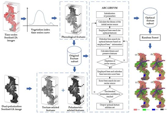
3.3. Experimental Workflow

Combining the advantages of time series Sentinel-2A and dual-polarization Sentinel-1A images, multiple features such as vegetation phenology parameters, polarimetric vegetation parameters, backscattering parameters, polarimetric decomposition parameters and texture features were extracted, and the optimal feature subset was selected using the ABC-LIBSVM algorithm. Finally, random forest classification was employed to classify the optimal feature subset, as a means to compare and analyze the extraction accuracy of the urban forests. A workflow of the study is given in Figure 4.

4. Results and Discussion

4.1. Optimal Feature Selection and Analysis

In this study, phenological parameters extracted from the time series vegetation index, and polarimetric and texture parameters extracted from Sentinel-1A were formed into a feature set. Particle swarm optimization using the LIBSVM (PSO-LIBSVM) algorithm and the improved artificial bee colony (ABC-LIBSVM) algorithm were used for feature selection, and the advantages and disadvantages of these two methods with respect to feature selection were compared. The optimal feature subsets selected by the two algorithms for describing urban forests are shown in

Table 2. Optimal feature subsets.

Feature Selection Algorithms	Feature Subset	Velocity Selection
PSO-LIBSVM (16)	EVNDVI, EVNDRE704, SINDRE704, ETNDRE740, SVNDRE740, EVNDRE740, BVNDRE740, AmpNDRE740, SVNDRE780, EVNDRE780, LINDRE780, STEVI, SIEVI, MAXVH, CONVV, HomVV	Slow (120 min)
ABC-LIBSVM (16)	ETNDVI, EVNDVI, LDNDVI, ETNDRE704, LINDRE704, LDNDRE704, AmpNDRE704, ETNDRE780, SVNDRE780, EVNDRE780, STEVI, EVEVI, LIEVI, MAXVV, VH, Alpha(α)	Fast (30 min)

.

It can be seen from Table 2 that the number of optimal features selected by PSO-LIBSVM and ABC-LIBSVM was the same, but the features were different. Further, the former took 120 min and the latter 30 min. Both methods pay attention to the description of forest using the end-of-growing-season value of NDVI (${\mathrm{EV}}_{\mathrm{NDVI}}$), the start- and end-of-growing-season values of ${\mathrm{NDRE}}_{780}$ (${\mathrm{SV}}_{{\mathrm{NDRE}}_{780}}$, ${\mathrm{EV}}_{{\mathrm{NDRE}}_{780}}$), the start-of-growing-season time value of EVI (${\mathrm{ST}}_{\mathrm{EVI}}$), the largest time integral (LI), and amplitude (Amp). Forests in Nanjing are mainly composed of evergreen and deciduous forests. While the leaves wither, the evergreen forest also keeps sprouting and remains evergreen for all four seasons. The difference is that crops and grasslands are withered and yellow at the end of the corresponding growth season, and large areas of soil are exposed to the surface, which has a certain impact on the acquisition of NDVI parameters. Therefore, the value of forest NDVI at the end of the growth period is more stable and reliable than that of other types of vegetation. Further, it can be seen from Figure 5a that the combination of the end-of-growth-season data of the three red-edge vegetation indices, ${\mathrm{NDRE}}_{704}$, ${\mathrm{NDRE}}_{740}$, and ${\mathrm{NDRE}}_{780}$, can be used to distinguish farmland from other vegetation, indicating that the addition of red-edge bands helps to separate urban forest from other vegetation, so as to improve the extraction accuracy.

Amplitude (Amp) represents the maximum difference of vegetation index between vegetation growth seasons. As the red-edge band has a good correlation with the vegetation density, the amplitude (Amp) extracted from the red-edge vegetation index is able to describe the difference in the growth density between the forest and other vegetation. According to the growth process of crops in Nanjing, there are almost no large areas of vegetation growth in the farmland before and after rice sowing. The sprouting distribution is sparse at the beginning of rice growth, and gradually thickens until the middle of the growth stage. Therefore, the amplitude exhibits an obvious difference between the sowing and the peak periods. The forests in the study area are mostly mixed forests with little difference in amplitude values, and can be easily distinguished from other land types such as farmland.

Time integration has the biological significance of vegetation productivity in a certain period of time, that is, the ability of vegetation to produce organic matter through photosynthesis. The study area has rich forest resources, and is the largest carbon pool in the regional ecosystem. Its productivity is much higher than that of rice, vegetable fields, and other crops planted in the suburbs of the city. Therefore, the parameter of largest time integration (LI) can be used to further distinguish forest from farmland. In addition, the LI parameter also represents vegetation productivity and photosynthetic capacity, which can be considered as an essential characteristic basis for monitoring the carbon storage and distribution of ecological resources in the future.

The effect of vegetation growth time on forest extraction was also considered using the ABC-LIBSVM feature selection method. Among the selected features, there were many parameters at the start and end (ST and ET) of the urban forest vegetation growth season, including the end growth time of NDVI and ${\mathrm{NDRE}}_{780}$, and the start growth time of EVI and ${\mathrm{NDRE}}_{704}$. As mentioned above, the forests in Nanjing are mixed forests, which are mainly deciduous forests supplemented by evergreen forests. Deciduous trees begin to sprout in March and April, and enter a vigorous growing season in May, during which the vegetation coverage becomes more luxuriant. In late October, the leaves turn yellow, and the deciduous trees enter the dormant period, and the forest density decreases. Compared with other vegetation at the same time, the density of urban forests is still at a high level, and can be easily perceived by the red-edge vegetation index. The growth law of crops is similar to that of deciduous forests. In the study area, the rice variety is mostly late-maturing mid-japonica, which is sown in mid-early May and matures in mid-late October. The whole growth period is 150–160 days. Compared with forest and rice, the vegetable growth cycle is shorter, generally 30 to 90 days. It can also be seen from Figure 5b that the urban forest samples were fault-distributed at the end of the growing season in the red-edge band, some evergreen vegetation was on the high value, and the other deciduous forest samples were close to the farmland samples due to their possessing similar growth laws. In summary, the vegetation coverage density of forest was generally higher than that of crops and other land types during the growth period. The red-edge band showed a good correlation between the leaf area and vegetation density. Therefore, the phenological parameters related to growth time extracted from multiple vegetation indices, such as the start- and end-of-growing-season, are beneficial for forest extraction.

The optimal feature subset selected by the PSO-LIBSVM algorithm includes the maximum probability texture value (MAX) of the VH channel and the contrast (Con) and homogeneity (Hom) of the VH channel. The ABC-LIBSVM algorithm is more inclined to select the polarimetric parameters themselves, such as VH and Alpha, to explore the fundamental difference between forest vegetation and crop vegetation from the scattering characteristics. According to the sample scatter in Figure 5c,d, it can be seen that, when only using the selected polarimetric and texture features of SAR data, urban forest cannot be distinguished from farmland, which also verifies that using only one type of remote sensing data cannot accurately describe the vegetation types.

On the basis of the above analysis of the growth law of the vegetation in this study area, it can be found that the two population algorithms train and select the same number of feature subsets that are conducive to describing the urban forest. On the other hand, it was also proved that combining multi-source remote sensing features, such as the phenology features from red-edge band, polarimetric and texture features from SAR can improve the accuracy of land cover classification and urban forest extraction. Further, the ABC-LIBSVM method has an advantage over the PSO method with respect to feature selection speed.

4.2. Classification Results

To explore the feasibility of the proposed method in remote sensing classification and further compare the advantages and disadvantages of ABC-LIBSVM and PSO-LIBSVM in feature selection, this research applied the random forest (RF) classifier to classify four different feature sets, and the classification confusion matrix was calculated to compare and analyze. Feature set 1 has 55 phenological parameters extracted from 5 optical vegetation indices. Feature set 2 is composed of 81 features, including all phenological features, polarimetric decomposition parameters, texture features, etc. Feature set 3 is a set of 16 feature parameters selected using the PSO-LIBSVM method. Feature set 4 is a set of 16 feature parameters selected by the ABC-LIBSVM algorithm presented in this study. As the urban grassland is scattered and can easily be covered by tall vegetation such as trees, it is difficult to distinguish the grassland in the low- and medium-resolution remote sensing images. Therefore, the landscape vegetation in the study area, including scenic forest, agricultural forest, shrub, grassland, and street trees, was regarded as urban forest. The land cover types can be divided into four categories: forests, urban, farm, and water. Figure 6 shows the classification results of the four feature sets, and Figure 7 shows the local area amplification results.

4.3. Discussion

PSO is an type of evolutionary algorithm for finding the optimal solution through cooperation and information sharing among individuals in the group [33,60]. It starts from a random solution, looks for an optimal solution through iteration, evaluates the quality of the solution through fitness, and searches for the global optimum on the basis of the current optimal value [61]. However, the PSO algorithm also has some problems, such as poor treatment of discrete optimization problems and ease of falling into local optima [62]. As another intelligent algorithm, the ABC algorithm (ABC) makes up for the local one-sidedness of the particle swarm algorithm when searching for the optimal solution, and systematically analyzes and searches for the optimal solution from a global perspective. In this paper, the wrapper feature selection method of ABC combined with LIBSVM has a strong global search ability, and can avoid the problems of fast convergence in PSO algorithm. At the same time, LIBSVM, as a strong support vector machine library, has multiple models to use. It also supports multi-category classification and has a wider application field. Compared with the traditional SVM, LIBSVM is more flexible and mature, and the results are more satisfactory. In this research, LIBSAM was introduced into the fitness solution of PSO and ABC, and the advantages and disadvantages of the two feature selection algorithms were compared, further verifying the necessity of multi-source feature combination.

By comparing high-resolution Google Earth images and field survey data, it can be seen from Figure 6a and Figure 7a that most urban forest areas can be correctly distinguished using feature set 1. The overall classification accuracy and kappa coefficient of feature set 1 were 81.47% and 0.7408, respectively, and the producer accuracy and user accuracy of the forest reached 79.90% and 79.07%, respectively. By comparing Figure 6b and

Table 3. Classification accuracy.

Classification (RF)		Forest	Farm	Urban	Water
Feature set 1	PA%	79.90	72.79	85.31	100.00
	UA%	79.07	81.72	73.94	90.04
	OA%	81.47
	Kappa Coefficient	0.7408
Feature set 2	PA%	82.38	78.14	70.98	99.31
	UA%	77.81	79.89	92.27	90.74
	OA%	82.47
	Kappa Coefficient	0.7508
Feature set 3	PA%	79.11	80.77	78.32	100.00
	UA%	81.02	80.50	88.89	89.86
	OA%	83.42
	Kappa Coefficient	0.7652
Feature set 4	PA%	93.21	78.25	81.82	96.77
	UA%	82.45	91.68	79.32	91.50
	OA%	86.80
	Kappa Coefficient	0.8145

, it can be observed that when the polarimetric- and texture-related features were introduced into the classification, the overall accuracy and kappa coefficient of the study area improved, but the range of improvement was very small. Compared with Google mapping, in the same area, the boundaries in results of feature set 2 were clearer and more intuitive than those of feature set 1. However, the producer accuracy of feature set 2 only increased by about 2.4% in forest extraction. From the yellow and blue boxes in Figure 7a,b, it was not difficult to see that some forest areas in the study area were mistakenly classified as farms and the former was more serious than the latter. This shows that the addition of relevant SAR features, such as polarimetric and texture features, can improve the overall results and the forest classification to a certain extent; however, the combination of too many features leads to information redundancy, which limits a significant improvement in the classification results.

The PSO-LIBSVM algorithm and the ABC-LIBSVM algorithm were used to select the best feature subset of the urban forest. The classification results using the selected optimal feature sets are displayed in Figure 6c,d. From local area amplification results (Figure 7c,d), it is clear that the feature set selected by ABC-LIBSVM method had less misclassification in urban forest. This may because that the proposed method can perform global search in the whole feature set to achieve the optimal features selection, and avoid falling into local optimization. The feasibility of this method in remote sensing feature selection was clearly proven. It can be seen from Table 3 that when performing classification using the random forest method, the results of both the feature set extracted by PSO-LIBSVM and the feature set extracted by ABC-LIBSVM were better than those obtained for feature set 1 (only optical phenological features) and feature set 2 (integrating all optical and SAR related features). The overall classification accuracy and kappa coefficient obtained by the PSO-LIBSVM algorithm were 83.42% and 0.7652, respectively, and these two indicators were 86.80% and 0.8145, respectively, for the ABC-LIBSVM algorithm. For urban forest, the user accuracy and producer accuracy of feature set 3 were lower than those of feature set 1 and 2, which may be because PSO-LIBSVM has the problems of weak search ability and excessive convergence speed, so the selected features were not comprehensive enough to accurately distinguish urban forests from other land cover types. It can also be seen from Table 3 that the forest’s user accuracy of feature set 4 was 13.31% higher than that of feature set 1, 10.83% higher than that of feature set 2, and 14.1% higher than that of feature set 3. The producer accuracy was 3.38%, 4.64%, and 1.43% higher, respectively, fully verifying the advantages of the improved ABC algorithm in urban forest remote sensing feature selection. Further, the comparisons also showed that the ABC-LIBSVM can not only can reduce the redundancy and interference between features, but can also fully mine multi-source remote sensing information, greatly improving the accuracy of urban forest classification, as well as the overall classification results. In addition, it was further shown that the features selected by the proposed method described the urban forest more accurately and efficiently than the PSO algorithm.

In conclusion, on the basis of the comparisons of multiple groups of experimental results, it is confirmed that the method of applying the LIBSVM-ABC algorithm to remote sensing feature selection to obtain high-precision land cover classification is applicable and feasible. This avoids the information redundancy and interference caused by the participation of too many features in classification, and it accelerates the speed of data processing. It was further verified that the combination of multi-source features was conducive to performing land cover classification and urban forest extraction.

5. Conclusions

To explore the potential of multi-source time series remote sensing features in urban forest information extraction, this study combined 55 phenological features extracted from time series Sentinel-2A optical data and 26 polarimetric- and texture-related features extracted from Sentinel-1A SAR data to form a multi-source feature set. Based on the proposed improved ABC method, the feature set was optimized and applied to urban classification and urban forest information extraction. The following conclusions can be drawn through the comparative analysis of the experiment:

(1)

By analyzing the state and time of vegetation in the growth season cycle, combined with Sentinel-1A and time series Sentinel-2A multi-source remote sensing data, multiple phenological parameters can be extracted, and the differences between forests and other vegetation can then be accurately distinguished from the perspective of phenology. The start time (ST) and value (SV) of vegetation growth season can help to distinguish forest vegetation from crops in the study area. The time integration reflects the vegetation productivity that can further distinguish forest from farmland. In addition, the amplitude (Amp) of the normalized vegetation index is able to describe the difference in the growth density between the forest and other vegetation. These phenological parameters improve the distinction between urban forests and other vegetation in different respects.

(2)

The ABC intelligence algorithm selects the features of the multi-source remote sensing feature set from a global perspective, avoiding the presence of too many features impacting the remote sensing classification results due to information redundancy, and also improving the optimal feature selection speed. The experimental results showed that the application of ABC-LIBSVM in remote sensing feature selection was feasible and was able to obtain better forest extraction and overall classification results. In this paper, the proposed feature selection algorithm was combined with random forest for Nanjing classification. The overall accuracy and the kappa coefficient were 86.80% and 0.8145, respectively. For the urban forest, the producer accuracy and the user accuracy were 93.21% and 82.45%, respectively. These indicators were higher than the results obtained for the PSO-LIBSVM feature selection method.

(3)

This study also verified the potential application of Sentinel-2A multispectral images and Sentinel-1A SAR image integration for urban land classification. After comparing the classification results of multi-source features with those of the single data source, it was found that the former had certain advantages in urban forest information extraction and overall accuracy improvement. In particular, after feature selection and the optimization of multi-source combined features, the classification results of all land cover types in the study area were improved, and the classification accuracy of forests was improved by more than 11%.

Overall, this paper studied urban land classification, especially forest information extraction, on the basis of different data sources integration, time series parameters extraction, feature selection, and other aspects, and satisfactory results were achieved. However, there are still some limitations to the current research, such as the fact that the amount of polarimetric SAR data used was small, and the image resolution was moderate, which may lead to the classification not being fine enough. In future research, we will consider adding terrain or full polarimetric data to further improve the accuracy of urban land classification and urban forest extraction, and we will also consider using the object-oriented segmentation algorithm to solve the salt and pepper problem caused by pixel classification.

References

1. Li, D.; Fan, S.; He, A.; Yin, F. Forest Resources and Environment in China. J. For. Res. 2004, 9, 307–312. [Google Scholar] [CrossRef]
2. Curtis, P.G.; Slay, C.M.; Harris, N.L.; Tyukavina, A.; Hansen, M.C. Classifying Drivers of Global Forest Loss. Science 2018, 361, 1108–1111. [Google Scholar] [CrossRef] [PubMed]
3. Pan, Y.; Birdsey, R.A.; Phillips, O.L.; Jackson, R.B. The Structure, Distribution, and Biomass of the World’s Forests. Annu. Rev. Ecol. Evol. Syst. 2013, 44, 593–622. [Google Scholar] [CrossRef]
4. Xia, C.; Huang, G.; Liu, X. Multi-scale remote sensing monitoring system facing forest resources supervision in China. In Proceedings of the IEEE International Geoscience and Remote Sensing Symposium (IGARSS), Munich, Germany, 22–27 July 2012; pp. 5955–5958. [Google Scholar]
5. Camarretta, N.; Harrison, P.A.; Bailey, T.; Potts, B.; Lucieer, A.; Davidson, N.; Hunt, M. Monitoring forest structure to guide adaptive management of forest restoration: A Review of Remote Sensing Approaches. New For. 2020, 51, 573–596. [Google Scholar] [CrossRef]
6. de Lima, R.P.; Marfurt, K. Convolutional Neural Network for Remote-Sensing Scene Classification: Transfer Learning Analysis. Remote Sens. 2020, 12, 86. [Google Scholar] [CrossRef]
7. Potapov, P.; Li, X.; Hernandez-Serna, A.; Tyukavina, A.; Hansen, M.C.; Kommareddy, A.; Pickens, A.; Turubanova, S.; Tang, H.; Silva, C.E.; et al. Mapping global forest canopy height through integration of GEDI and Landsat data. Remote Sens. Environ. 2021, 253, 112165. [Google Scholar] [CrossRef]
8. Segarra, J.; Buchaillot, M.L.; Araus, J.L.; Kefauver, S.C. Remote sensing for precision agriculture: Sentinel-2 improved features and applications. Agronomy 2020, 10, 641. [Google Scholar] [CrossRef]
9. Phiri, D.; Simwanda, M.; Salekin, S.; Nyirenda, V.R.; Murayama, Y.; Ranagalage, M. Sentinel-2 data for land cover/Use mapping: A review. Remote Sens. 2020, 12, 2291. [Google Scholar] [CrossRef]
10. Zhang, H.; Zhu, J.; Wang, C.; Lin, H.; Long, J.; Zhao, L.; Fu, H.; Liu, Z. Forest growing stock volume estimation in subtropical mountain areas using PALSAR-2 L-Band PolSAR data. Forests 2019, 10, 276. [Google Scholar] [CrossRef]
11. Kumar, S.; Garg, R.D.; Govil, H.; Kushwaha, S.P.S. PolSAR decomposition based extended water cloud modeling for forest aboveground biomass estimation. Remote Sens. 2019, 11, 2287. [Google Scholar] [CrossRef] [Green Version]
12. Ferrentino, E.; Nunziata, F.; Zhang, H.; Migliaccio, M. On the Ability of PolSAR measurements to discriminate among mangrove species. IEEE J. Sel. Top. Appl. Earth Obs. Remote Sens. 2020, 13, 2729–2737. [Google Scholar] [CrossRef]
13. Li, W.; Chen, E.; Li, Z.; Luo, H.; Zhou, W.; Feng, Q.; Wang, X. Combing polarization coherence tomography and polinsar segmentation for forest above ground biomass estimation. In Proceedings of the IEEE International Geoscience and Remote Sensing Symposium (IGARSS), Munich, Germany, 22–27 July 2012; pp. 3351–3354. [Google Scholar]
14. Yu, Y.; Li, M.; Fu, Y. Forest type identification by random forest classification combined with SPOT and multitemporal SAR data. J. For. Res. 2018, 29, 1407–1414. [Google Scholar] [CrossRef]
15. Zhou, J.; Chen, J.; Chen, X.; Zhu, X.; Qiu, Y.; Song, H.; Rao, Y.; Zhang, C.; Cao, X.; Cui, X. Sensitivity of six typical spatiotemporal fusion methods to different influential factors: A comparative study for a normalized difference vegetation index time series reconstruction. Remote Sens. Environ. 2021, 252, 112130. [Google Scholar] [CrossRef]
16. Huang, J.; Tian, L.; Liang, S.; Ma, H.; Becker-Reshef, I.; Huang, Y.; Su, W.; Zhang, X.; Zhu, D.; Wu, W. Improving winter wheat yield estimation by assimilation of the leaf area index from Landsat TM and MODIS data into the WOFOST model. Agric. For. Meteorol. 2015, 204, 106–121. [Google Scholar] [CrossRef]
17. Vrieling, A.; Meroni, M.; Darvishzadeh, R.; Skidmore, A.K.; Wang, T.; Zurita-Milla, R.; Oosterbeek, K.; O’Connor, B.; Paganini, M. Vegetation phenology from Sentinel-2 and field cameras for a dutch barrier island. Remote Sens. Environ. 2018, 215, 517–529. [Google Scholar] [CrossRef]
18. Bargiel, D. A new method for crop classification combining time series of radar images and crop phenology information. Remote Sens. Environ. 2017, 198, 369–383. [Google Scholar] [CrossRef]
19. Zeng, L.; Wardlow, B.D.; Xiang, D.; Hu, S.; Li, D. A review of vegetation phenological metrics extraction using time-series, multispectral satellitedata. Remote Sens. Environ. 2020, 237, 111511. [Google Scholar]
20. Bai, B.; Tan, Y.; Guo, D.; Xu, B. Dynamic monitoring of forest land in fuling district based on multi-source time series remote sensing images. ISPRS Int. J. Geo-Inf. 2019, 8, 36. [Google Scholar] [CrossRef]
21. Maus, V.; Camara, G.; Cartaxo, R.; Sanchez, A.; Ramos, F.M.; de Queiroz, G.R. A time-weighted dynamic time warping method for land-use and land-cover mapping. IEEE J. Sel. Top. Appl. Earth Obs. Remote Sens. 2016, 9, 3729–3739. [Google Scholar] [CrossRef]
22. Belgiu, M.; Csillik, O. Sentinel-2 cropland mapping using pixel-based and object-based time-weighted dynamic time warping analysis. Remote Sens. Environ. 2018, 204, 509–523. [Google Scholar]
23. Jia, K.; Liang, S.; Zhang, L.; Wei, X.; Yao, Y.; Xie, X. Forest cover classification using Landsat ETM plus data and time series MODIS NDVI data. Int. J. Appl. Earth Obs. Geo-Inf. 2014, 33, 32–38. [Google Scholar]
24. Soudani, K.; Delpierre, N.; Berveiller, D.; Hmimina, G.; Vincent, G.; Morfin, A.; Dufrene, E. Potential of C-Band synthetic aperture radar Sentinel-1 time-series for the monitoring of phenological cycles in a deciduous forest. Int. J. Appl. Earth Obs. Geo-Inf. 2021, 104, 102505. [Google Scholar] [CrossRef]
25. Antropov, O.; Rauste, Y.; Hame, T.; Praks, J. Polarimetric ALOS PALSAR time series in mapping biomass of boreal forests. Remote Sens. 2017, 9, 999. [Google Scholar] [CrossRef] [Green Version]
26. Luo, Q.; Xing, W.; Qiming, X. Identification of pests and diseases of dalbergia hainanensis based on EVI time series and classification of decision tree. IOP Conf. Ser. Earth Environ. Sci. 2017, 69, 012162. [Google Scholar] [CrossRef]
27. Uddin, M.P.; Mamun, M.A.; Afjal, M.I.; Hossain, M.A. Feature selection with segmentation-based folded Principal Component Analysis (PCA) for hyperspectral image classification. Int. J. Remote Sens. 2021, 42, 286–321. [Google Scholar] [CrossRef]
28. Zhao, J.; Pan, X.; Tang, Z.; Du, J.; Yin, S.; He, L.; Li, R. (Eds.) Remote sensing image feature selection based on rough set Theory and Multi-Agent system. In Proceedings of the 12th International Conference on Fuzzy Systems and Knowledge Discovery (FSKD), Zhangjiajie, China, 15–17 August 2015; pp. 705–709. [Google Scholar]
29. Luo, M.; Wang, Y.; Xie, Y.; Zhou, L.; Qiao, J.; Qiu, S.; Sun, Y. Combination of feature selection and CatBoost for prediction: The first application to the estimation of aboveground biomass. Forests 2021, 12, 216. [Google Scholar] [CrossRef]
30. Georganos, S.; Grippa, T.; Vanhuysse, S.; Lennert, M.; Shimoni, M.; Kalogirou, S.; Wolff, E. Less Is More: Optimizing classification performance through feature selection in a very-high-resolution remote sensing object-based urban application. GIsci. Remote Sens. 2018, 55, 221–242. [Google Scholar] [CrossRef]
31. Agrawal, P.; Abutarboush, H.F.; Ganesh, T.; Mohamed, A.W. Metaheuristic algorithms on feature selection: A survey of one decade of research (2009–2019). IEEE Access 2021, 9, 26766–26791. [Google Scholar]
32. Sarmadian, A.; Moghimi, A.; Amani, M.; Mahdavi, S. Optimizing the snake model using honey-bee mating algorithm for road extraction from very high-resolution satellite images. In Proceedings of the 2022 10th International Conference on Agro-geoinformatics (Agro-Geoinformatics), Québec, QC, Canada, 11 July 2022; pp. 1–6. [Google Scholar]
33. Ghamisi, P.; Benediktsson, J.A. Feature selection based on hybridization of genetic algorithm and Particle Swarm Optimization. IEEE Geosci. Remote Sens. Lett. 2015, 12, 309–313. [Google Scholar] [CrossRef]
34. Saboori, M.; Homayouni, S.; Shah-Hosseini, R.; Zhang, Y. Optimum feature and classifier selection for accurate urban land use/cover mapping from very high resolution satellite imagery. Remote Sens. 2022, 14, 2097. [Google Scholar] [CrossRef]
35. Neagoe, V.-E.; Neghina, C.-E. An Artificial Bee Colony approach for classification of remote sensing imagery. In Proceedings of the 10th International Conference on Electronics, Computers and Artificial Intelligence (ECAI), Iași, Romania, 28–30 June 2018; pp. 1–4. [Google Scholar]
36. Yi, Y.; He, R. A novel Artificial Bee Colony algorithm. In Proceedings of the 6th International Conference on Intelligent Human-Machine Systems and Cybernetics (IHMSC), Hangzhou, China, 26–27 August 2014; pp. 271–274. [Google Scholar]
37. Garcia-Balboa, J.L.; Alba-Fernandez, M.V.; Ariza-Lopez, F.J.; Rodriguez-Avi, J. Analysis of Thematic Similarity Using Confusion Matrices. ISPRS Int. J. Geo-Inf. 2018, 7, 233. [Google Scholar] [CrossRef]
38. Fernandez-Manso, A.; Fernandez-Manso, O.; Quintano, C. Sentinel-2A red-edge spectral indices suitability for discriminating burn severity. Int. J. Appl. Earth Obs. Geo-Inf. 2016, 50, 170–175. [Google Scholar] [CrossRef]
39. Ren, J.; Chen, Z.; Yang, X.; Liu, X.; Zhou, Q. Regional yield prediction of winter wheat based on retrieval of leaf area index by remote sensing technology. In Proceedings of the IEEE International Geoscience and Remote Sensing Symposium (IGARSS), Cape Town, South Africa, 12–17 July 2009; pp. 374–377. [Google Scholar]
40. Duan, S.; He, H.S.; Spetich, M. Effects of growing-season drought on phenology and productivity in the west region of central hardwood forests, USA. Forests 2018, 9, 377. [Google Scholar] [CrossRef]
41. Zhao, L.; Xing, X.; Zhang, P.; Ma, X.; Pan, Z.; Cui, N. Land cover classification based on daily normalized difference vegetation index time series from multitemporal remotely sensed data. Fresenius Environ. Bull. 2020, 29, 2029–2040. [Google Scholar]
42. Liu, J.; Zhan, P. The impacts of smoothing methods for time-series remote sensing data on crop phenology extraction. In Proceedings of the IEEE International Geoscience and Remote Sensing Symposium (IGARSS), Beijing, China, 10–15 July 2016; pp. 2296–2299. [Google Scholar]
43. Pastor-Guzman, J.; Dash, J.; Atkinson, P.M. Remote sensing of mangrove forest phenology and its environmental drivers. Remote Sens. Environ. 2018, 205, 71–84. [Google Scholar]
44. Atkinson, P.M.; Jeganathan, C.; Dash, J.; Atzberger, C. Inter-comparison of four models for smoothing satellite sensor time-series data to estimate vegetation phenology. Remote Sens. Environ. 2012, 123, 400–417. [Google Scholar] [CrossRef]
45. Li, M.; Bijker, W. Potential of multi-temporal Sentinel-1A dual polarization SAR images for vegetable classification in Indonwsia. In Proceedings of the IEEE International Geoscience and Remote Sensing Symposium (IGARSS), Valencia, Spain, 22–27 July 2018; pp. 3820–3823. [Google Scholar]
46. Koyama, C.N.; Watanabe, M.; Shimada, M. Monitoring of soil moisture dynamics in the semi-arid tropics by means of ALOS-2/PALSAR-2 dual-polarization scansar data. In Proceedings of the IEEE International Geoscience and Remote Sensing Symposium (IGARSS), Valencia, Spain, 22–27 July 2018; pp. 5513–5516. [Google Scholar]
47. Li, M.; Bijker, W. Vegetable classification in indonesia using dynamic time warping of Sentinel-1A dual polarization SAR time series. Int. J. Appl. Earth Obs. Geo-Inf. 2019, 78, 268–280. [Google Scholar] [CrossRef]
48. Phruksahiran, N. Potential performance of polarimetric reference function of SAR data processing by coherent target decomposition. Signal Image Video Process. 2021, 15, 1021–1029. [Google Scholar] [CrossRef]
49. Ainsworth, T.L.; Wang, Y.; Lee, J.-S. Model-based polarimetric SAR decomposition: An L-1 regularization approach. IEEE Trans. Geosci. Remote Sens. 2022, 60, 1–13. [Google Scholar] [CrossRef]
50. An, W.; Lin, M.; Yang, H. Modified reflection symmetrydecomposition and a new polarimetric product of GF-3. IEEE Geosci. Remote Sens. Lett. 2022, 19, 1–5. [Google Scholar]
51. Jiao, Y.; Guo, Z.; Ye, S.; DEStech Publicat, I. Research on classification of remote sensing image based on Grey Level Co-Occurrence Matrix and BP Neural Network. In Proceedings of the International Conference on GIS and Resource Management (ICGRM), Guangzhou, China, 3–5 January 2014; pp. 29–35. [Google Scholar]
52. Zhang, X.; Cui, J.; Wang, W.; Lin, C. A study for texture feature extraction of high-resolution satellite images based on a direction measure and gray level Co-Occurrence matrix fusion algorithm. Sensors 2017, 17, 1474. [Google Scholar] [CrossRef]
53. Huang, X.; Zhang, L. An SVM ensemble approach combining spectral, structural, and semantic features for the classification of high-resolution remotely sensed imagery. IEEE Trans. Geosci. Remote Sens. 2013, 51, 257–272. [Google Scholar] [CrossRef]
54. Szigarski, C.; Jagdhuber, T.; Baur, M.; Thiel, C.; Parrens, M.; Wigneron, J.-P.; Piles, M.; Entekhabi, D. Analysis of the Radar Vegetation Index and Potential Improvements. Remote Sens. 2018, 10, 1776. [Google Scholar] [CrossRef]
55. Mandal, D.; Bhattacharya, A.; Kumar, V.; Ratha, D.; Dey, S.; McNairn, H.; Frery, A.C.; Rao, Y.S. A novel radar vegetation index for compact polarimetric SAR data. In Proceedings of the IEEE International Geoscience and Remote Sensing Symposium (IGARSS), Yokohama, Japan, 28 July–2 August 2019; pp. 1037–1040. [Google Scholar]
56. Yadav, V.P.; Prasad, R.; Bala, R.; Srivastava, P.K.; Vanama, V.S.K. Appraisal of dual polarimetric radar vegetation index in first order microwave scattering algorithm using Sentinel-1A (C—Band) and ALOS-2 (L—Band) SAR data. Geocarto Int. 2021, 37, 6232–6250. [Google Scholar] [CrossRef]
57. Mandal, D.; Kumar, V.; Ratha, D.; Dey, S.; Bhattacharya, A.; Lopez-Sanchez, J.M.; McNairn, H.; Rao, Y.S. Dual polarimetric radar vegetation index for crop growth monitoring using Sentinel-1 SAR data. Remote Sens. Environ. 2020, 247, 111954. [Google Scholar] [CrossRef]
58. Chang, C.-C.; Lin, C.-J. LIBSVM: A Library for Support Vector Machines. ACM Trans. Intell. Syst. Technol. 2011, 2, 1–27. [Google Scholar] [CrossRef]
59. Leiva, L.; Vazquez, M.; Torrents-Barrena, J. FPGA Acceleration analysis of LibSVM predictors based on high-level synthesis. J. Supercomput. 2022, 78, 14137–14163. [Google Scholar] [CrossRef]
60. Chen, W.-N.; Tan, D.-Z. Set-based discrete Particle Swarm Optimization and its applications: A Survey. Front. Comput. Sci. 2018, 12, 203–216. [Google Scholar] [CrossRef]
61. Zhang, Y.; Wang, S.; Ji, G. A comprehensive survey on Particle Swarm Optimization Algorithm and its applications. Math. Probl. Eng. 2015, 2015, 931256. [Google Scholar] [CrossRef]
62. Lalwani, S.; Sharma, H.; Satapathy, S.C.; Deep, K.; Bansal, J.C. A survey on Parallel Particle Swarm Optimization Algorithms. Arab. J. Sci. Eng. 2019, 44, 2899–2923. [Google Scholar] [CrossRef]
Figure 1. Geographical location of the study area.
Remotesensing 14 04859 g001
Figure 2. The schematic diagram of vegetation index time series curve.
Remotesensing 14 04859 g002
Figure 3. Workflow of the ABC-LIBSVM algorithm for feature selection.
Remotesensing 14 04859 g003
Figure 4. Experimental workflow.
Remotesensing 14 04859 g004
Figure 5. Scatter plot of farm and forest in different parameter spaces: (a) spatial scatter plot of NDRE 704 / NDRE 740 / NDRE 780 ; (b) spatial scatter plot of NDRE 704 / NDVI / NDRE 780 ; (c) spatial scatter plot of MAX VH / Con VV / Hom VV ; and (d) spatial scatter plot of MAX VV /VH/α.
Remotesensing 14 04859 g005
Figure 6. Classification results: (a) results of feature set 1; (b) results of feature set 2; (c) results of feature set 3; and (d) results of feature set 4.
Remotesensing 14 04859 g006
Figure 7. Local area amplification results: (a) feature set 1; (b) feature set 2; (c) feature set 3; and (d) feature set 4.
Remotesensing 14 04859 g007