Time-Series Evolution Patterns of Land Subsidence in the Eastern Beijing Plain, China
by
Junjie Zuo
1,2, 
Huili Gong
1,2,
Beibei Chen
1,2,*,
Kaisi Liu
1,2,
Chaofan Zhou
1,2 and
Yinghai Ke
1,2 1
Base of the Key Laboratory of Urban Environmental Process and Digital Modeling, Capital Normal University, Beijing 100048, China
2
College of Resources Environment and Tourism, Capital Normal University, Beijing 100048, China
*
Author to whom correspondence should be addressed.
Remote Sens. 2019, 11(5), 539; https://doi.org/10.3390/rs11050539
Submission received: 4 January 2019
/
Revised: 25 February 2019
/
Accepted: 26 February 2019
/
Published: 5 March 2019
(This article belongs to the Special Issue Advances in Remote Sensing-based Disaster Monitoring and Assessment)
Abstract
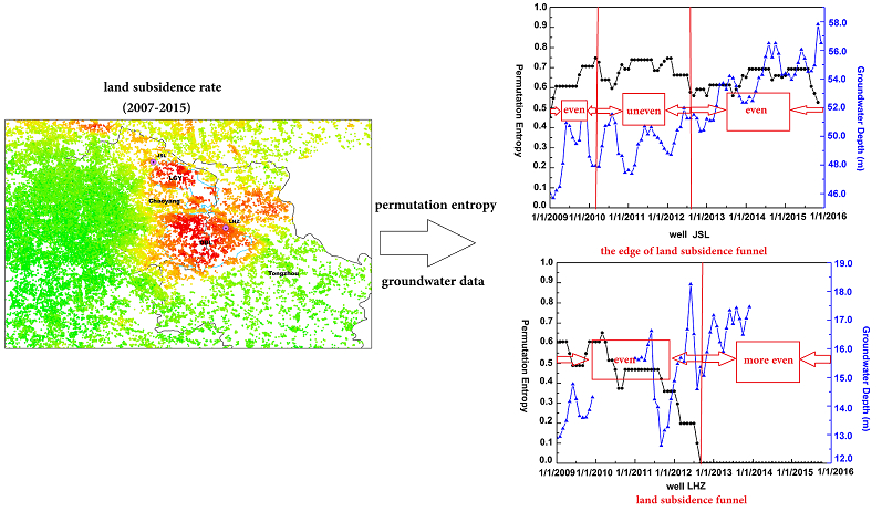
:Land subsidence in the Eastern Beijing Plain has a long history and is always serious. In this paper, we consider the time-series evolution patterns of the eastern of Beijing Plain. First, we use the Persistent Scatterer Interferometric Synthetic Aperture Radar (PSI) technique, with Envisat and Radarsat-2 data, to monitor the deformation of Beijing Plain from 2007 to 2015. Second, we adopt the standard deviation ellipse (SDE) method, combined with hydrogeological data, to analyze the spatial evolution patterns of land subsidence. The results suggest that land subsidence developed mainly in the northwest–southeast direction until 2012 and then expanded in all directions. This process corresponds to the expansion of the groundwater cone of depression range after 2012, although subsidence is restricted by geological conditions. Then, we use the permutation entropy (PE) algorithm to reverse the temporal evolution pattern of land subsidence, and interpret the causes of the phenomenon in combination with groundwater level change data. The results show that the time-series evolution pattern of the land subsidence funnel edge can be divided into three stages. From 2009 to 2010, the land subsidence development was uneven. From 2010 to 2012, the land subsidence development was relatively even. From 2012 to 2013, the development of land subsidence became uneven. However, subsidence within the land subsidence funnel is divided into two stages. From 2009 to 2012, the land subsidence tended to be even, and from 2012 to 2015, the land subsidence was relatively more even. The main reason for the different time-series evolution patterns at these two locations is the annual groundwater level variations. The larger the variation range of groundwater is, the higher the corresponding PE value, which means the development of the land subsidence tends to be uneven.

1. Introduction
During the last few decades, interferometric synthetic aperture radar (InSAR) has become an important tool for the mapping and monitoring deformation processes [1,2,3,4]. With the InSAR technique, we can measure deformation over a large scale, from millimeters to centimeters. However, this method faces the problems of spatial and temporal decorrelation and atmospheric distribution. Persistent Scatterers InSAR (PSI) was proposed to overcome the limitations of InSAR [5,6]. The PSI techniques has shown its potential for ground deformation monitoring in a number of applications, including land subsidence [7,8,9,10], seismic faults [11,12,13], and landslide-prone slopes [14,15,16].
Since the 1960s, land subsidence has been found in the Beijing Plain, which has experienced rapid development. Currently, land subsidence is extremely uneven, and it has formed two major settlements centers in the north and south. The north settlement center has become the largest ground settlement funnel group on the Beijing Plain. Many scholars study the spatiotemporal evolution characteristics of the settlement on the Beijing Plain. The studies indicate that the deformation has mainly occurred in the eastern and northern part of the Beijing Plain, and Chaoyang and the northeastern part of Tongzhou have experienced the most severe subsidence. Land subsidence shows an increasing trends in the rate and extent over time [17,18,19,20,21]. The uneven settlement has developed rapidly, and the changes in land subsidence in the north–south direction are more pronounced than those in other directions [22]. The deformation of the Beijing Plain shows seasonal variations, and the spatial location of land subsidence funnels is consistent with the location of the groundwater cone of depression, although not entirely [23]. The spatial distribution of the deformation rate from 2003 to 2010 was similar to that from 2010 to 2016, but the subsidence rate from 2010 to 2016 was higher that from 2003 to 2010 [24].
Most of these studies focus on the spatial distribution of land subsidence, however, fewer studies examine the time-series evolution pattern. In this paper, we pay attention to the time series of the land subsidence pattern. First we use the standard deviation ellipse (SDE) method to reveal the spatial evolution pattern of land subsidence; then we adopt the permutation entropy (PE) algorithm in order to determine how the land subsidence changes over time. PE is a complex parameter based on the comparison of adjacent data in a long time series. It amplifies the imperceptible changes in the signal by quantitatively describing the variations in signal spatial complexity [25,26]. This complexity shows a difference. PE mainly compares the differences between the variations in settlement data in the former time interval and those in the latter time interval. PE monitors the differences in the land subsidence process in a long time series. More specifically, the difference reflects whether land subsidence develops uniformly or not in the long time series. The process of PE value increase is the process of increasing difference in land subsidence, which means land subsidence develops more unevenly over this period of time. The process of PE value decrease is the process of decreasing difference in land subsidence, which means land subsidence develops more evenly during this time. At present, many scholars who have studied the PE method. The main applications of this method include medicine, biology, climate, and image processing [27,28,29,30]. Most scholars approximately analyze the overall development of deformation in the whole research period through the time-series settlement. Using the PE method, we can reveal the different development processes of subsidence with time. PE amplifies the settlement details, which are hard to determine using other methods.
This paper is organized as follows. The background of the study area and datasets used are described in Section 2. The data methods are presented in Section 3. In Section 4, we use the SDE method combined with the changes in the land subsidence funnel area, in the center of gravity, and in the spatial distribution and range to reveal the spatial evolution pattern of land subsidence. Meanwhile, we adopt the PE method to respond to the time-series evolution pattern. In Section 5, we discuss the relationship between the spatial evolution pattern obtained by SDE and hydrogeologic data. Moreover, we explore the causes of the different PE results for the land subsidence funnel and funnel edge and find that this phenomenon is mainly due to the difference in the annual variations in the groundwater level.
2. Study Area and Dataset
2.1. Study Area
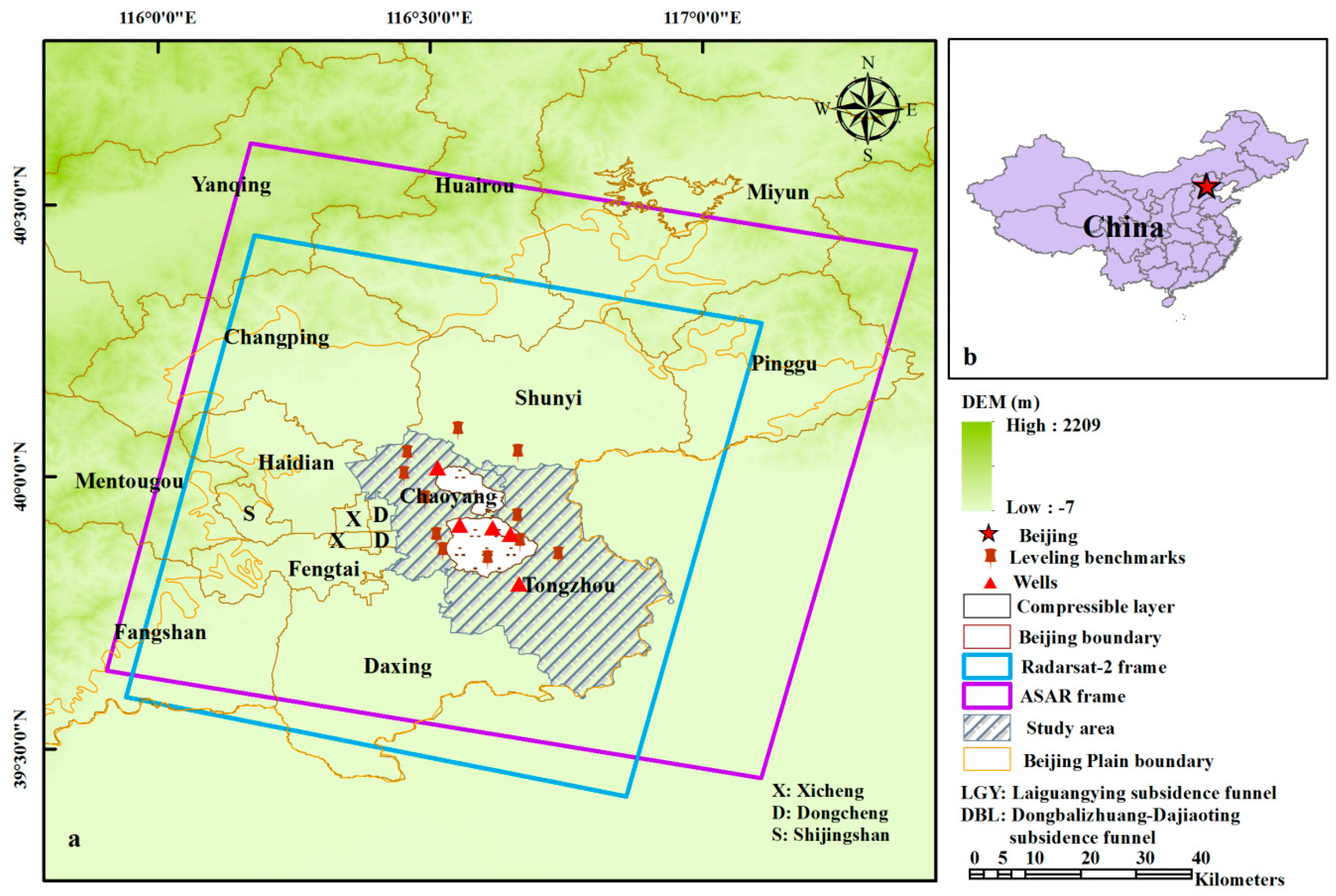
The study area (Figure 1) is located in the eastern part of the Beijing Plain, which is an area with serious land subsidence and a part of the warm temperate zone, with a semihumid and semiarid continental monsoon climate and an annual average temperature of 11–12 °C. The precipitation distribution in the study area is extremely uneven. The precipitation in summer is approximately 70% of the annual precipitation, which is much higher than that in winter [31].
The groundwater system in the study area is composed of three water systems. They are the Yongding River system, Wenyu River system, and Chaobai River system. According to the groundwater supplementation, diameter, drainage conditions, groundwater exploitation horizon, and genesis type, the Quaternary aquifers in the study area are mainly divided into three main aquifer groups [19,23]. The first group of aquifers is in Holocene and upper Pleistocene strata, which are widely distributed. The depth of the floor is 35–75 m and it is a multilayer structure. The underground water types include upper stagnant water, interlayer water, diving, and shallow confined water. The lithologies includes fine sand, silt, silty sand, and sandy clay. The second aquifer group is the middle Pleistocene strata. The types of groundwater mainly include variations in the shallow groundwater level in the study area, which is mainly affected by the precipitation infiltration of medium and deep confined water. The alluvial-diluvial fan floor of the Yongding River is buried as deep as 150 m and that of the Chaobai River is as deep as 190 m. The lithologies include multiple types of gravel, sand, and clay soil. The last aquifer group is in the lower Pleistocene strata, which are composed of medium coarse and gray sand. The water-bearing group is distributed in the middle and lower parts of the alluvial–diluvial fan with a multilayer structure. The groundwater type is mainly deep confined water, and the roof is buried as deep as 190 m.
2.2. Dataset
The dataset used in this study comes from two different satellites. One set is the 31 C bands descending track ASAR images acquired from January 2007 to August 2010, with a 35 day revisit cycle, which was provided by the European Space Agency. The other set is the 48 C bands Radarsat-2 images acquired from Oct. 2010 to Nov.2015, with a 24 day revisit cycle, which was provided by the Canadian Space Agency. The spatial resolutions of both Envisat ASAR and Radarsat-2 images were 30 m. The coverage of the SAR images is shown in Figure 1, and the detailed parameters of the SAR images are summarized in Table 1.
We use the SARPROZ software to handle our SAR images. And we use the Shuttle Radar Topography Mission (SRTM) digital elevation model (DEM) with a spatial resolution of 90 m to remove the topographic phase and to geocode interferograms. The groundwater level contours are provided by the Beijing Water Authority and are used for comparing the relationship between the groundwater levels and subsidence, and the well locations are shown in Figure 1a.
3. Methods
3.1. PSI Method
The Persistent Scatterer Interferometric Synthetic Aperture Radar (PSI) was proposed by Ferretti [5]. The technique reduces the incoherence and atmospheric effects in the time and space domains. It is capable of extracting the targets points with a strong and stable radiometric property, and of obtaining surface deformation by separating the topographic phase of the ground targets. In this study, we use the SARPROZ software to acquire the surface deformation information for the study area.
The surface deformation phase can be obtained using the PSI procedure by decomposing the interferometric phase based on Equation (1):
where is the interferometric phase, and is the flat earth phase, which can be removed by the precise orbital state vector of the satellite, obtained using the SARPROZ software, when reading SAR images. is the topographic phase contributed by the topographic relief, and it can be removed by the external DEM in the SARPROZ software; is the deformation phase caused by the displacement of the ground during the two image acquisitions. What we truly would like to obtain is the . is the atmospheric phase due to the contribution of atmospheric components, and APS processing in the SARPROZ software can eliminate this phase. is the thermal noise and coregistration errors, which can be removed by the linear models in APS processing. However, is the deformation phase in the radar line-of-sight (LOS) direction including the horizontal and vertical directions. Hence, the LOS () can be converted into vertical displacement () by the following Equation (2):
where θ is the incidence angle.
3.2. Standard Deviation Ellipse Method
The standard deviation ellipse (SDE) method was first proposed by Lefever in 1926 to analyze the spatial distribution characteristics of discrete datasets [32]. In this study, we use numerous parameters of SDE, such as the ellipse center, long axis, and short axis, to analyze the spatial characteristics of land subsidence. These parameters can be calculated as follows:
where and are the coordinates of PSI points, is the mean center of PSI points, and n is the total number of PSI points. The rotation angle is calculated as follows:
where and are the deviation of and the mean center, respectively. The standard deviations of the X and Y axes are given by:
where is the azimuth of the ellipse, indicating the direction of the north clockwise rotation angle to the long axis of the ellipse, is the standard deviation of the X axis and is the standard deviation of the Y axis.
3.3. Permutation Entropy Method
Christoph Bandt et al. [25], proposed an entropy parameter to measure the complexity of the one-dimensional time series, called the permutation entropy (PE). It is similar to the LyaPullov index in terms of performance reflecting one-dimensional time-series complexity. However, compared with complex parameters such as the LyaPullov index and fractal dimension, PE has the characteristics of simpler calculation and stronger anti-noise interference ability.
Given a land subsidence time series , for various n, n increasing to ∞ [25], any of the elements is a phase space reconstruction of the elements , and then the following is obtained:
In Equation (6), m and l are the embedded dimension and delay time, respectively. The m components of are rearranged as:
If exists, these values are sorted by the size of the j value at this time. This step means when , then . Thus, any vector can produce a sequence of symbols:
In Equation (8), where , and , there are kinds of different arrangements of m different symbols, which indicates that there are kinds of symbol sequences. The symbol sequence of is one example. The occurrence probability of each symbol, such as is calculated. Hence, the k kinds of symbol sequences of the time series can be defined in the form of the Shannon information entropy:
When , is up to the maximum value . For convenience, usually can be labeled as:
The value of indicates the degree of randomness of the time series . The smaller the value of is, the more regular of the time series; the higher the value of is, the more random of the time series. With the various values of , pamplifies the small variations in the time series .
In this paper, we use the MATLAB software to realize the PE method. Because the study period is relatively short (only nine years), we choose three embedded dimensions, and the delay time is two years, which indicates that the cumulative land subsidence for the first two years is a training sample. The sliding window step size is one, which ensures that the variations in the PE are due to the changes in the state of settlement at the later time nodes.
4. Results
4.1. Land Subsidence Information Monitoring by PSI Validation
The Eastern Beijing Plain has two major deformation bowls, which are named the Laiguangying (LGY) and Dongbalizhuang-Dajiaoting (DBL) land subsidence funnels. They are the places with the earliest and most serious subsidence in Beijing, and the two subsidence funnels have been developing since they were discovered in 1983 (Figure 1). The two subsidence funnels are located in Chaoyang and Tongzhou Districts, respectively. Chaoyang is the industrial base of Beijing, and Tongzhou is the subcenter of Beijing. Meanwhile, these districts are key areas for future planning and construction in Beijing, including of the Central Business District (CBD), in the CBD east expansion zone. Hence, understanding the spatial and temporal evolution of land subsidence in these two regions is important for the urban development of Beijing.
We selected 11 leveling points in 2009, which were chosen to verify the PSI processing results (Figure 2). In 2009, the maximum error of the two measurements was 19.91 mm, and the minimum error was 1.18 mm. The error is caused by the deviation between the position of the PSI point and the position of the leveling point. However, the correlation coefficient between the leveling point and the PSI points is 0.94, which proves that the two sets of points show good consistency. The PSI monitoring results are reliable.
4.2. Spatial Evolution Pattern by the SDE Method
The SDE is an effective approach, which can accurately reveal the geographical spatial distributions and other characteristics using spatial statistical methods. We use the annual land subsidence rate as the weight and adopt the spatial analysis method to obtain the SDE. Figure 3 shows the cumulative land subsidence information and SDE shapes from 2007 and 2015 in the study area. The maximum accumulated land subsidence reached 1.184 m by 2015. We can observe that land subsidence was serious and the spatial distribution of land subsidence increased with time. The major axis of the SDE is oriented northwest–southeast. This position reflects that the development of land subsidence in the northwest–southeast direction is more obvious than those in other directions. We take the annual subsidence of 60 mm as the dividing line and define the place with more than 60 mm as the subsidence funnel areas. We find that after 2008, the LGY and DBL land subsidence funnels evolves into a single area. We describe the spatial distribution of land subsidence in the eastern part of Beijing Plain with respect to the following four factors: the changes in the land subsidence funnel area; the changes in the center of gravity of land subsidence; the changes in the distribution range of land subsidence and the changes in the distribution of land subsidence.
4.2.1. Changes in the land subsidence funnel area
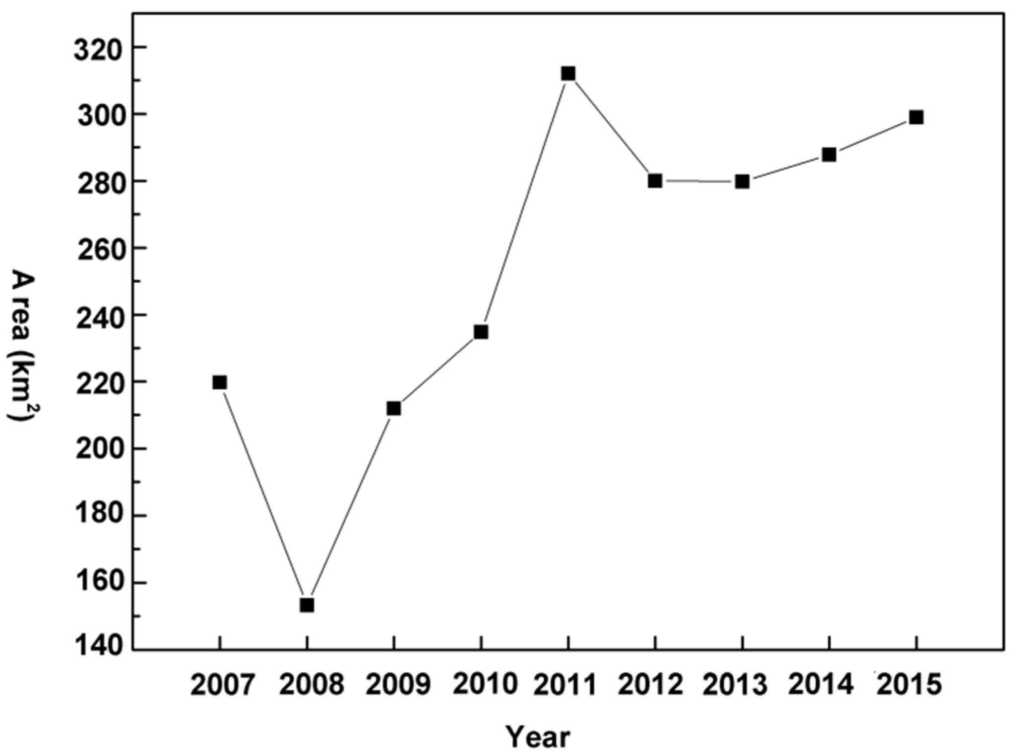
We calculated the area of the land subsidence funnels from 2007 to 2015 (Figure 4). From Figure 4, we can see the land subsidence funnel area was 253.28 km2 in 2008, which was the smallest value and accounted for 10.97% of the total study area. The land subsidence funnel area was 312.04 km2 in 2011, which was the greatest value and accounted for 21.79% of the total study area. From 2007 to 2008, the land subsidence funnel area decreased; then, it continued to increase rapidly until 2011, especially from 2008 to 2009 and 2010 to 2011. Between 2011 and 2012, the area decreased, and from 2012 to 2015, the area increased slowly. Therefore, we can find that the area of land subsidence in the study area is still increasing, but the growth rate of the area has been lower, especially since 2012. This result means that land subsidence in the study area is still slowly developing.
4.2.2. Changes in the center of the gravity of land subsidence
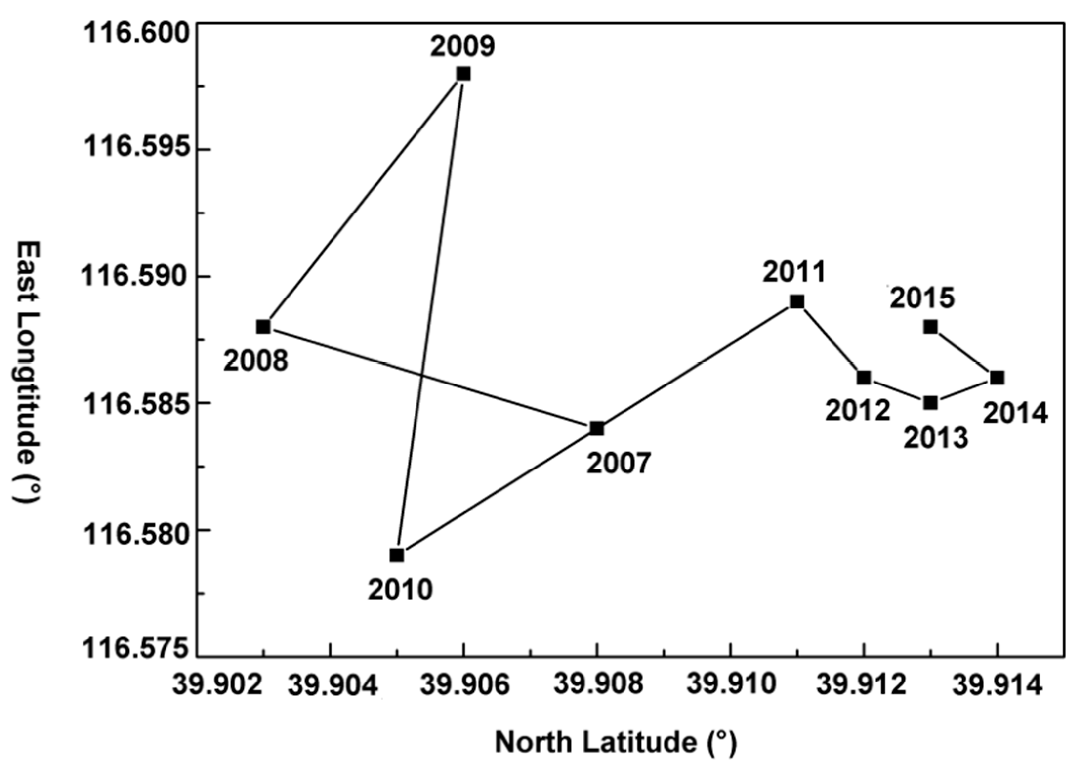
The changes in the central migration trajectory of SDE from 2007 to 2015 are shown in Figure 5. We find that the central coordinates of the SDE in 2007 were 116.584° E, 39.908° N and those in 2015 were 116.588° E, 39.913° N. The center of the SDE of the study area moved toward the northeast as a whole. From 2007 to 2008, the center moved to the southeast; in 2008 and 2009, it moved to the northeast; between 2009 and 2010, it moved to the southwest; between 2010 and 2014, it moved to the north; and from 2014 to 2015, it moved to the southeast. Combining this information with that in Figure 2, the SDE center of the study area has been changing toward the direction of the northern part of the DBL land subsidence funnel. We estimate that this land subsidence funnel will still be the land subsidence development center of the Chaoyang and Tongzhou Districts.
4.2.3. Changes in the distribution range of land subsidence
The length of the long axis of the SDE represents the distribution range of land subsidence. The spatial variation distributions of land subsidence in the study area from 2007 to 2015 is shown in Figure 6. The long axis decreased from 154.438 m in 2007 to 119.448 m in 2015. From 2007 to 2008, the long axis increased, suggesting that the spatial distribution range of land subsidence increased. Combining this information with that in Figure 4, we can see that the land subsidence funnel area was decreasing during this period, which means that the distribution of land subsidence was dispersed. From 2008 to 2012, the long axis decreased rapidly, indicating that the distribution range of land subsidence was reduced during this period. However, the land subsidence funnel area expanded in 2008 and 2012, which indicated that the land subsidence of the area was concentrated; meanwhile, land subsidence showed a tendency to merge into one region during this time. From 2012 to 2015, the long axis was increasing slowly, which indicated that the distribution range of land subsidence was increasing. The area of the land subsidence funnel expanded, indicating that land subsidence increased during this time.
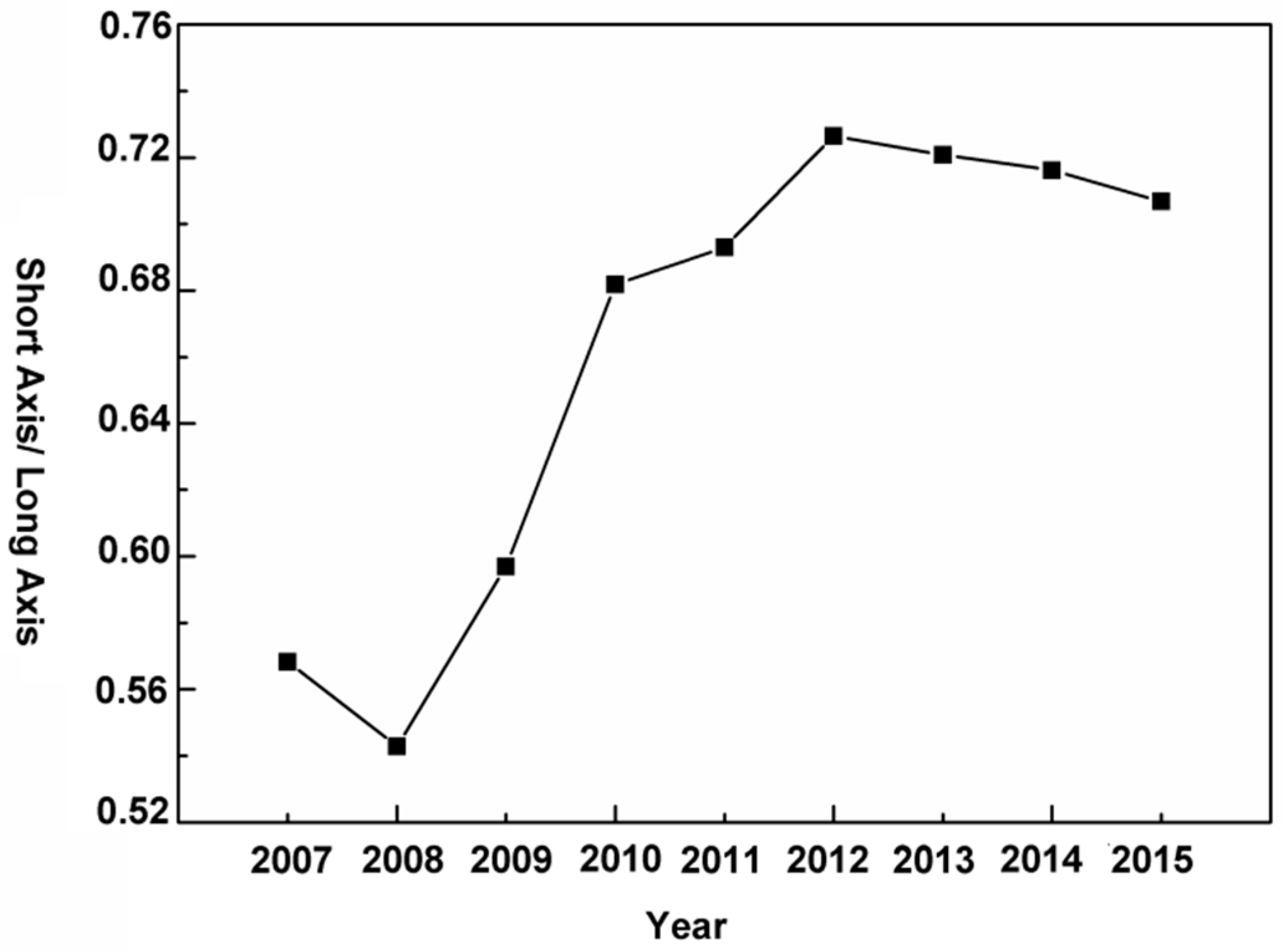
4.2.4. Changes in the distribution of land subsidence
The ratio of the short axis to the long axis of the SDE represents the spatial distribution shape of land subsidence. When the ratio is close to 1, the spatial distribution shape of land subsidence is close to a circle. That is, land subsidence evolves more uniformly in all directions. The spatial distribution shape changes in the study area are shown in Figure 7. From 2007 to 2015, the spatial distribution shape changed significantly. Between 2007 and 2008, the ratio of the short axis to the long axis decreased, which means that land subsidence mainly changed toward the long axis in the northwest–southeast direction. From 2008 to 2012, the ratio of the two axes increased rapidly, suggesting that during this period, land subsidence intensified in the short axis direction (northeast–southwest direction). Between 2012 and 2015, the ratio of the two axes decreased slowly, indicating that land subsidence was relatively uniform in all directions during this time. In short, the main direction of land subsidence development was in the northwest–southeast direction before 2008. After 2008, land subsidence intensified in the northeast–southwest direction and showed a trend of expansion.
4.3. Temporal Evolution Pattern by the PE Method
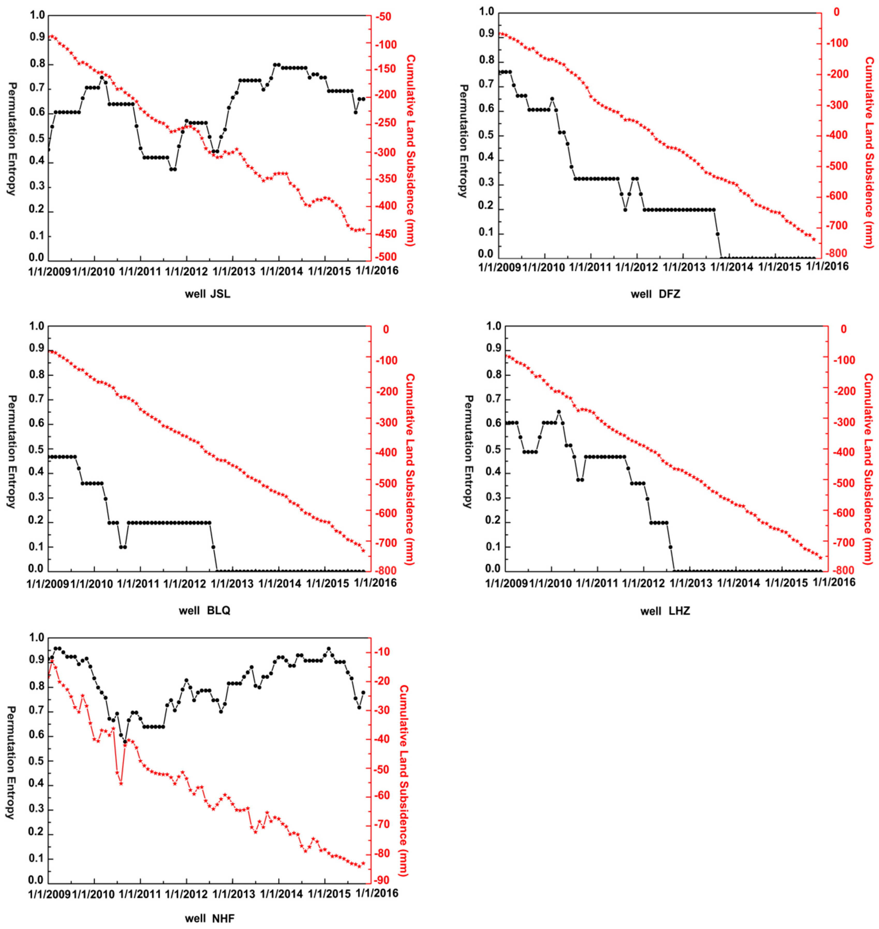
According to the LGY and DBL land subsidence funnel cumulative deformation rate, we selected five wells and analyzed the time-series evolution pattern of land subsidence in the deformation funnels and funnel edges using the PE method. The results are shown in Figure 8.
The PE results for well JSL are shown in Figure 8a. JSL lies at the edge of the LGY subsidence funnel area. The cumulative land subsidence ranged from −50–450 mm between 2007 and 2015. It showed a linear increasing trend from 2009 to 2010. After 2012, it showed an increasing trend with volatility. In contrast to the PE result, since 2009, the PE value of JSL was increasing and reached a maximum in April 2010. This phenomenon indicates that the land subsidence development was relatively uneven during the period from 2009 to April 2010. The value continued to decrease from April 2010 to October 2011, and it reached a minimum value in October 2011. This phenomenon indicates that the state of the land subsidence development developed from a nonuniform state to a uniform state during this period. After October 2011, the PE value increased, which means that land subsidence developed toward a nonuniform state.
The PE results for well DFZ are shown in Figure 8b. DFZ belongs to the DBL subsidence funnel. The cumulative land subsidence varied from 0 to −740 mm from 2007 to 2015. The cumulative land subsidence showed a downward trend. However, the PE value continued decreasing from 2009 to November 2013. This phenomenon indicates that land subsidence tended to develop toward a uniform state after 2009. The value returned to zero during the period from November 2013 to 2015. This result means that after this time, the cumulative land subsidence continued to increase, with no decrease. This result indicates that the land subsidence in DFZ has been in a more uniform state since 2013.
The PE results for well BLQ are shown in Figure 8c. BLQ is located in the DBL subsidence funnel. The cumulative land subsidence ranged from 0 to −740 mm between 2007 and 2015. The cumulative land subsidence showed a linear rise in the study period. The PE value decreased from 2009, and the minimum value appeared in August 2012. Then, in the following years, the value was zero. In other words, land subsidence was moving toward a uniform trend from 2009 to 2012. In addition, after 2012, the cumulative land subsidence continued to increase, which indicates that the land subsidence of this well will was relatively more uniform.
The PE results for well LHZ are shown in Figure 8d. LHZ lies in the DBL subsidence funnel. During the research period, the cumulative settlement was increasing linearly. The PE value, decreased form 2009, until August 2012, when it reached its minimum. This result indicates that land subsidence moved from a nonuniform state to a uniform state. After August 2012, the PE value became zero, which showed that the state of land subsidence development was more uniform than that in August 2012. This result reflected that the value of cumulative land subsidence was progressively increasing.
The PE results for well NHF are shown in Figure 8e. NHF is located at the edge of the DBL subsidence funnel. The cumulative land subsidence ranged from 20 to −90 mm during the period from 2007 to 2015, with fluctuations. The value of PE increased from the beginning of January 2009 to April 2009. This phenomenon reflected that in this period, the development of land subsidence was uneven. From April 2009 to July 2011, the value decreased significantly, which means that the development of land subsidence in during this period trended to be even. The value increased between July 2011 and 2015, which indicates that land subsidence developed unevenly.
According to the value of the PE, the development of land subsidence at the edge of the funnel is different from that within the land subsidence funnel. The PE results at the edge of the funnel increased first, then decreased, and finally increased, indicating that land subsidence developed nonuniformly first, then uniformly, and nonuniform again during the research period. However, since 2009, the value of PE for land subsidence decreased during the research period; even after 2012, the value was even zero. This phenomenon indicates that, since 2009, land subsidence at these three wells trended to be uniform. It became relatively more uniform after 2012.
Thus, based on the PE results, the state of land subsidence development at the edge of the land subsidence funnel can be divided into three stages. The first stage was from 2009 to 2010, when the PE value increased, which indicated that the land subsidence tended to be nonuniform. The second stage was from 2010 to 2012, when the value of PE decreased, implying that land subsidence developed from a nonuniform to a uniform state. In the third stage, from 2012 to 2015, the PE value increased, indicating that land subsidence developed in a uniform state. The state of land subsidence development in the land subsidence funnel can be arranged in two phases. During the first stage, the value of PE continually decreased between 2009 and 2012, which means that land subsidence developed uniformly in this period. The second stage was from 2012 to 2015, when the PE value returned to zero. This state indicates that the land subsidence during this period developed more uniformly than it had during the previous period.
5. Discussion
5.1. Relationship Between the Spatial Evolution Pattern by the SDE Method and Hydrogeologic Data
Combining the groundwater level contours and compressible sediment layer of the study area from 2007 to 2015 with the SDE obtained by PSI during the period, the correlation between the subsidence response patterns and the phreatic groundwater flow field was analyzed comprehensively (Figure 9). Comparing the groundwater levels of 2015 with the 2007 levels shows that the groundwater level declined by 15–25 m throughout the eastern part of the Beijing Plain.
When referring to the SDE, we find that it outlined two subsidence funnels. As times passed, the extent of land subsidence in the northwest–southeast direction expanded after 2012; then, the SDE started to develop in this direction. The expansion of land subsidence distribution was due to the groundwater cone of depression. In 2007, the groundwater elevations varied from 10 to 20 m, and there was a groundwater cone of depression in the LGY subsidence funnel. As time passed, the groundwater contours in this area became more compact, as in 2015. This result means that the groundwater consumption increased greatly. The LGY groundwater cone of depression expanded after 2012, and correspondingly, the rate and range of land subsidence in this area increased. The DBL subsidence funnel was not in the zone of the groundwater cone of depression bowl. However, land subsidence in this area achieved a maximum value, and the deformation increased from 2007 to 2015. This effect may have occurred due to soil consolidation, which causes hysteresis in the groundwater.
The stratum structure of the Beijing Plain is characterized by a transformation from a single structure zone to a multilayered structure zone from the northwest to the southeast. The sediment particles changed from coarse to fine, the thickness gradually increases, and the proportion of clay soil increases gradually [33]. Note that the thickness of the loose Quaternary sediments in the study area ranges from 80 to 210 m. The thickness of the compressible clay layer in LGY varies from 130 to 220 m and the thickness changed from 110 to 180 m in DBL. Meanwhile, land subsidence in these two areas achieved the maximum values. This result means that the spatial distribution of land subsidence and the thickness of the compressible sediment layer are significantly correlated. The greater the cumulative thickness of the sediment layer is, the greater the total land subsidence.
From comprehensive groundwater and compressible soil data, we find that the spatial evolution characteristics of land subsidence in the Eastern Beijing Plain are basically consistent with those of groundwater, although subsidence is restricted by geological conditions. The compressible soil layer provides the environment for land subsidence and the overexploitation of groundwater is the main cause of land subsidence.
5.2. Relationship Between the Temporal Evolution Pattern by the PE Method and Groundwater
From the permutation entropy results, we show that the results differed between the land subsidence funnel and the edge of the funnel. Combining this information with the land subsidence rates, we can discover that the cumulative land subsidence rate at the edge of the land subsidence funnel fluctuated after 2012, while the cumulative land subsidence rate in the land subsidence funnel was increasing during this time. The PE describes the differences in the cumulative settlements. Thus, these differences show that the PE is reliable.
As we know, the overextraction of groundwater is the main cause of settlement in the Beijing Plain. Hence, comprehensive groundwater level variation data are used to discover the relationship between the PE variations and groundwater level changes.
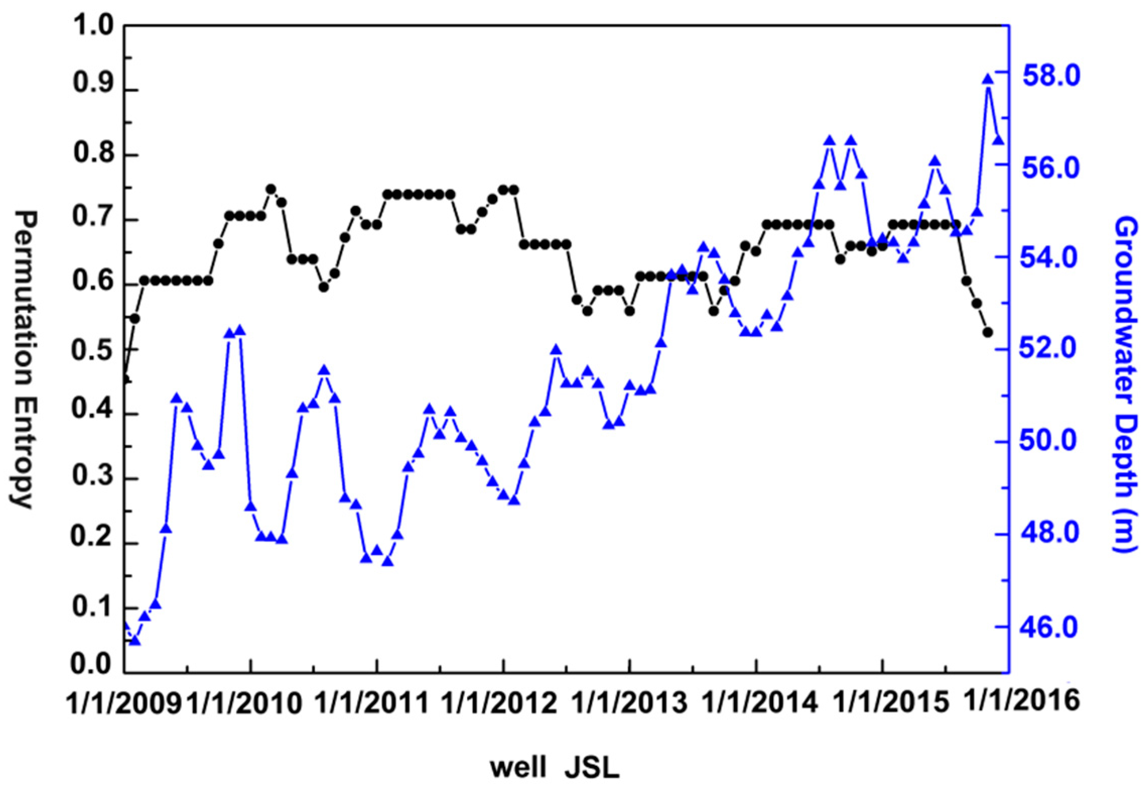
Only well JSL obtained groundwater level variation data from 2011 to 2015. Therefore, JSL was selected to analyze the relationship between the changes in the groundwater level and the PE results (Figure 10). The average annual variations in the groundwater level in well JSL were 6.71 m, 3.46 m and 3.6m between 2009 and 2010, from 2010 to 2012, and from 2012 to 2015, respectively. Combining the groundwater data with the PE results, indicates that between 2009 and 2010, the average annual variation in groundwater was greater than that between 2010 and 2012, while the average annual variation in the groundwater was smaller than that between 2012 and 2015. These results lead to the conclusion that the average annual settlement fluctuation was more pronounced between 2009 and 2010 than between 2010 and 2012. Meanwhile, the average annual settlement fluctuation was less pronounced between 2010 and 2012 than between 2012 and 2015. Therefore, the development of the accumulative settlement between 2009 and 2010 was more uneven than that between 2010 and 2012. In addition, the development of the cumulative settlement between 2010 and 2012 was more uniform than that between 2012 and 2015. This phenomenon corresponds to the process of the PE value increasing between 2009 and 2010 and decreasing between 2010 and 2012. This feature also explains, why PE increased between 2012 and 2015.
Wells DFZ, BLQ, and LHZ lie within the settlement funnel area of the research area, but BLQ acquired the groundwater level variation data only from 2009 to 2013. Therefore, DFZ and LHZ are selected to analyze the relationship between the variation in the groundwater level and the PE results (Figure 11, Figure 12).
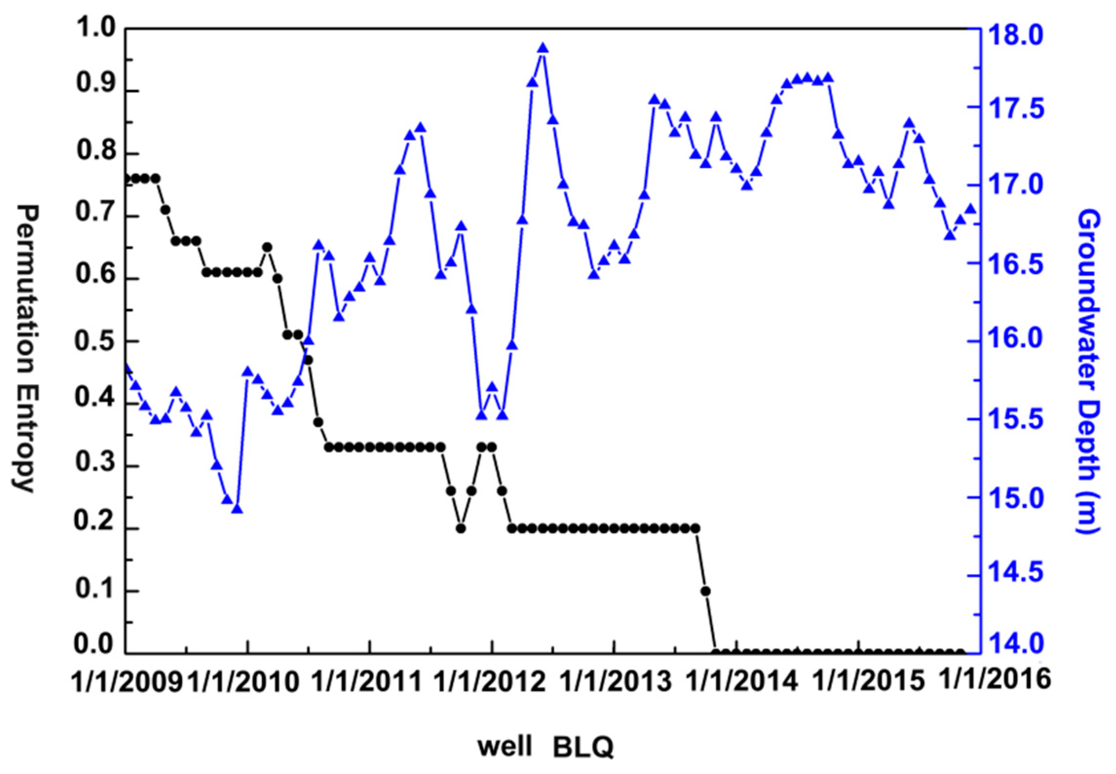
Figure 11 reveals the groundwater level variations in well BLQ. The average annual variation in the groundwater level in well BLQ was 1.51 m between 2009 and 2012, and the groundwater level average annual variation was 0.81 m between 2013 and 2015. Thus, the fluctuation in the groundwater level between 2009 and 2012 was almost twice that between 2013 and 2015. This result indicates that the settlement changes at well BLQ between 2009 and 2012 were faster than those between 2013 and 2015. Therefore, the PE value decreased. However, the groundwater fluctuation between 2013 and 2015 was less than 1 m per year. Thus, during this period, the land subsidence rate fluctuated little, and the accumulative land subsidence showed a slow increase. This result is expressed by the PE value returning to zero.
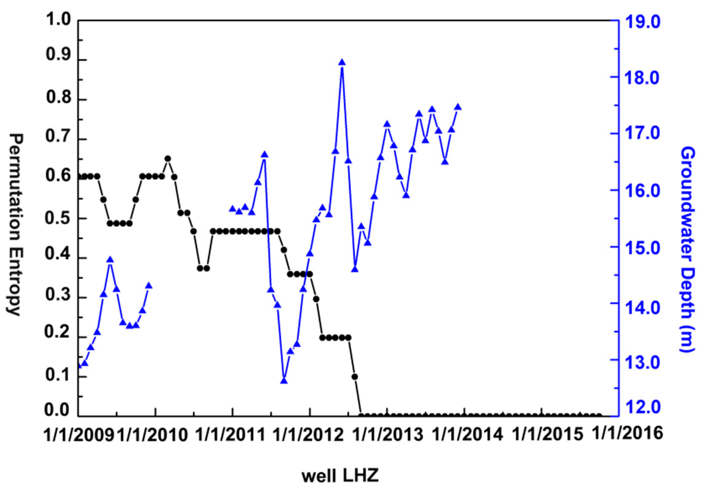
Figure 12 shows the groundwater level variations in well LHZ. During the period from 2011 to 2012, the groundwater level fluctuated greatly, and the average annual variation in groundwater in this period was 3.83 m. The average annual change in the groundwater level was 1.51 m between 2013 and 2015. From the above results, the groundwater level variation between 2011 and 2012 was more than twice that between 2013 and 2015. This result proves that the fluctuation in the land subsidence rate changed more quickly between 2011 and 2012 than that between 2013 and 2015, which means that between 2011 and 2012, the PE value is greater than that between 2013 and 2015. Thus, this process reflected the PE value decreasing. After 2013, the changes in groundwater were much smaller. Then, the land subsidence rate showed little fluctuation. Hence, the cumulative settlement continued slowly decreasing, which is expressed by the PE value becoming zero.
The groundwater level variation data for the three wells clearly show that the PE value for JSL was higher than those for DFZ and LHZ during the entire research time. This effect occurred because the average annual change of groundwater in JSL was greater than 3 m, while the average annual groundwater variation levels in DFZ and LHZ were approximately 1 m during the research period.
In summary, the groundwater level change is the main reason for why PE value for the five typical wells differ and the groundwater level changes correlate with the variations in PE values. The larger the variation range of groundwater is, the higher the corresponding PE value.
6. Conclusions
In this work, based on Envisat and Radarsat-2 data from 2007 to 2015, we detect the spatial and temporal evolution patterns of the two most serious land subsidence funnels in the Beijing Plain based on the SDE and PE methods. Integrating hydrogeological data, we conclude that the expansion of the groundwater cone of depression led to the development of the SDE in all directions after 2012. Moreover, the differences in the annual variations in the groundwater levels are the main reason for the different PE values of the land subsidence funnel and the funnel edge.
First, we utilize the PSI technique to obtain the long-term displacement in the Eastern Beijing Plain, China. The vertical displacement rates agree well with the measurements from ground leveling surveys: the correlation coefficient is 0.94, which indicates that our PSI results are reliable.
Then, we adopt the SDE to analyze the spatial evolution pattern of land subsidence. The SDE results suggest that the development of land subsidence in the southeast-northwest direction is more obvious than those in other directions; however, land subsidence develops obviously in all directions after 2012. Land subsidence is serious, and the spatial distribution of land subsidence increases over time. However, after 2012, the rate of increase of land subsidence decreases. Comparing the spatial evolution pattern using the SDE methods with the groundwater level changes and compressible sediment thicknesses, we find that the groundwater cone of depression expands and the range increases after 2012. At the same time, the compressible sediment thickness in the SDE range is large, providing an environment for land subsidence.
Finally, we use the PE method to reveal the time-series evolution pattern of land subsidence, and the results show that the time-series evolution pattern at the edge of the land subsidence funnel is different from that within the land subsidence funnel. The settlement development process at the edge of the land subsidence funnel is divided into three stages. From 2009 to 2010, the land subsidence development is uneven. From 2010 to 2012, the land subsidence development is relatively uniform. From 2012 to 2015, the development of land subsidence becomes nonuniform. We divide the land subsidence development of the land subsidence funnel into two stages. From 2009 to 2012, land subsidence tends to be uniform. From 2012 to 2015, land subsidence is more even than that in the previous period. Comparing the PE results with the groundwater level change data, the value of the PE increase corresponds to the process of increase in the groundwater level variations. This result indicates that the process whereby land subsidence tends to be nonuniform. Conversely, the value of PE decreases, corresponding to the process of decrease in the groundwater level variation. This result shows that the process whereby land subsidence tends to be uniform. The larger the variation range of the groundwater is, the higher the corresponding PE value.
In this paper, we use the PE method to discover the temporal evolution process of deformation which can help us to better understand land subsidence. In the future, we will decompose the effects of the groundwater on land subsidence to determine more details.
Author Contributions
J.Z. performed the experiments, analyzed the data and wrote the paper. H.G. and B.C. provided crucial guidance and support through the research. K.L. and C.Z. processed the data. Y.K. made important suggestions on writing the paper.
Acknowledgments
This work was funded by the National Natural Science Foundation of China (number 41771455/D010702; 41401493), the Beijing Outstanding Young Scientist Project, the Beijing Natural Science Foundation (8182013), the China Postdoctoral Science Foundation (2018M641407), Beijing Youth Top Talent Project, the program of Beijing Scholars, and the National “Double-Class” Construction of University Projects, Capacity Building for Sci-Tech Innovation-Fundamental Scientific Research Funds(025185305000/194). Thanks for the excellent software package SARPROZ.
Conflicts of Interest
The authors declare no conflict of interest.
References
- Wright, T.J.; Parsons, B.E.; Lu, Z. Toward mapping surface deformation in three dimensions using InSAR. Geophys. Res. Lett. 2004, 31, 169–178. [Google Scholar] [CrossRef]
- Lohman, R.B.; Simons, M. Some thoughts on the use of InSAR data to constrain models of surface deformation: Noise structure and data downsampling. Geochem. Geophys. Geosyst. 2013, 6. [Google Scholar] [CrossRef]
- Chaussard, E.; Wdowinski, S.; Cabral-Cano, E.; Amelung, F. Land subsidence in central Mexico detected by ALOS InSAR time-series. Remote Sens. Environ. 2014, 140, 94–106. [Google Scholar] [CrossRef]
- Eriksen, H.Ø.; Lauknes, T.R.; Larsen, Y.; Corner, G.D.; Bergh, S.G.; Dehls, J.; Kierulf, H.P. Visualizing and interpreting surface displacement patterns on unstable slopes using multi-geometry satellite SAR interferometry (2D InSAR). Remote Sens. Environ. 2017, 191, 297–312. [Google Scholar] [CrossRef]
- Ferretti, A.; Prati, C.; Rocca, F. Nonlinear subsidence rate estimation using permanent scatterers in differential SAR interferometry. IEEE Trans. Geosci. Remote Sens. 2000, 38, 2202–2212. [Google Scholar] [CrossRef]
- Ferretti, A.; Colesanti, C.; Prati, C.; Rocca, F. Radar permanent scatterers identification in urban areas: Target characterization and sub-pixel analysis. In Proceedings of the IEEE Remote Sensing and Data Fusion Over Urban Areas, IEEE/isprs Joint Workshop, Rome, Italy, 8–9 November 2001; p. 52. [Google Scholar]
- Gong, H.; Zhang, Y.; Li, X.; Lu, X.; Chen, B.; Gu, Z. Land subsidence research in Beijing based on the Permanent Scatterers InSAR technology. Prog. Nat. Sci. 2009, 19, 1261–1266. [Google Scholar]
- Ng, A.H.; Ge, L.; Li, X.; Abidin, H.Z.; Andreas, H.; Zhang, K. Mapping land subsidence in Jakarta, Indonesia using persistent scatterer interferometry (PSI) technique with ALOS PALSAR. Int. J. Appl. Earth Obs. Geoinf. 2012, 18, 232–242. [Google Scholar] [CrossRef]
- Chaussard, E.; Amelung, F.; Abidin, H.; Hong, S.H. Sinking cities in Indonesia: ALOS PALSAR detects rapid subsidence due to groundwater and gas extraction. Remote Sens. Environ. 2013, 128, 150–161. [Google Scholar] [CrossRef]
- Raspini, F.; Loupasakis, C.; Rozos, D.; Adam, N.; Moretti, S. Ground subsidence phenomena in the Delta municipality region (Northern Greece): Geotechnical modeling and validation with Persistent Scatterer Interferometry. Int. J. Appl. Earth Obs. Geoinf. 2014, 28, 78–89. [Google Scholar] [CrossRef] [Green Version]
- Salvi, S.; Atzori, S.; Tolomei, C.; Antonioli, A.; Trasatti, E.; Merryman Boncori, J.P.; Pezzo, G.; Coletta, A.; Zoffoli, S. Results from INSAR monitoring of the 2010–2011 New Zealand seismic sequence: EA detection and earthquake triggering. In Proceedings of the IEEE International Geoscience and Remote Sensing Symposium, Munich, Germany, 22–27 July 2012; pp. 3544–3547. [Google Scholar]
- Champenois, J.; Fruneau, B.; Pathier, E.; Deffontaines, B.; Lin, K.-C.; Hu, J.-C. Monitoring of active tectonic deformations in the Longitudinal Valley (eastern Taiwan) using Persistent Scatterer InSAR method with ALOS PALSAR data. Earth Planet. Sci. Lett. 2012, 337, 144–155. [Google Scholar] [CrossRef]
- Krishnan, S.P.V.; Kim, D.; Jung, J. Subsidence in the Kathmandu Basin, before and after the 2015 Mw 7.8 Gorkha Earthquake, Nepal Revealed from Small Baseline Subset-DInSAR Analysis. GISci. Remote Sens. 2018, 55, 604–621. [Google Scholar]
- Farina, P.; Colombo, D.; Fumagalli, A.; Marks, F.; Moretti, S. Permanent Scatterers for landslide investigations: Outcomes from the ESASLAM project. Eng. Geol. 2006, 88, 200–217. [Google Scholar] [CrossRef]
- Mikhailov, V.; Kiseleva, E.; Smolyaninova, E.; Golubev, V.; Dmitriev, P.; Isaev, Y.; Dorokhin, K.; Hooper, A.; Esfahany, S.; Hanssen, R.; Khairetdinov, S. PS-InSAR Monitoring of Landslides in The Great Caucasus, Russia, Using Envisat, ALOS And TerraSAR-X SAR Images. In Proceedings of the ESA Living Planet Symposium, Edinburgh, United Kingdom, 9–13 September 2013; p. 283. [Google Scholar]
- Kiseleva, E.; Mikhailov, V.; Smolyaninova, E.; Dmitriev, P.; Golubev, V.; Timoshkina, E.; Hooper, A.; Samiei-Esfahany, S.; Hanssen, R. PS-InSAR Monitoring of Landslide Activity in the Black Sea Coast of the Caucasus. Procedia Technol. 2014, 16, 404–413. [Google Scholar] [CrossRef] [Green Version]
- Zhu, L.; Gong, H.; Li, X.; Wang, R.; Chen, B.; Dai, Z.; Teatini, P. Land subsidence due to groundwater withdrawal in the northern Beijing plain, China. Eng. Geol. 2015, 193, 243–255. [Google Scholar] [CrossRef]
- Chen, B.; Gong, H.; Li, X.; Lei, K.; Gao, M.; Zhou, C.; Ke, Y. Spatial–temporal evolution patterns of land subsidence with different situation of space utilization. Nat. Hazards 2015, 77, 1765–1783. [Google Scholar] [CrossRef]
- Chen, M.; Tomás, R.; Li, Z.; Motagh, M.; Li, T.; Hu, L.; Gong, H.; Li, X.; Yu, J.; Gong, X. Imaging Land Subsidence Induced by Groundwater Extraction in Beijing (China) Using Satellite Radar Interferometry. Remote Sens. 2016, 8, 468. [Google Scholar] [CrossRef]
- Zhang, Y.; Wu, H.A.; Kang, Y.; Zhu, C. Ground Subsidence in the Beijing-Tianjin-Hebei Region from 1992 to 2014 Revealed by Multiple SAR Stacks. Remote Sens. 2016, 8, 675. [Google Scholar] [CrossRef]
- Zhou, C.; Gong, H.; Zhang, Y.; Warner, T.; Wang, C. Spatiotemporal Evolution of Land Subsidence in the Beijing Plain 2003–2015 Using Persistent Scatterer Interferometry (PSI) with Multi-Source SAR Data. Remote Sens. 2018, 10, 552. [Google Scholar] [CrossRef]
- Zhou, C.; Gong, H.; Chen, B.; Guo, L.; Gao, M.; Chen, W.; Liang, Y.; Si, Y.; Wang, J.; Zhang, X. Spatiotemporal characteristics of land subsidence in Beijing from small baseline subset interferometric synthetic aperture radar and standard deviational ellipse. In Proceedings of the International Workshop on Earth Observation and Remote Sensing Applications, Guangzhou, China, 4–6 July 2016; pp. 78–82. [Google Scholar]
- Chen, B.; Gong, H.; Li, X.; Lei, K.; Zhu, L.; Gao, M.; Zhou, C. Characterization and causes of land subsidence in Beijing, China. Int. J. Remote Sens. 2017, 38, 808–826. [Google Scholar] [CrossRef]
- Yang, Q.; Ke, Y.; Zhang, D.; Chen, B.; Gong, H.; Lv, M.; Zhu, L.; Li, X. Multi-Scale Analysis of the Relationship between Land Subsidence and Buildings: A Case Study in an Eastern Beijing Urban Area Using the PS-InSAR Technique. Remote Sens. 2018, 10, 1006. [Google Scholar] [CrossRef]
- Bandt, C.; Pompe, B. Permutation entropy: A natural complexity measure for time series. Phys. Rev. Lett. 2002, 88, 1–4. [Google Scholar] [CrossRef] [PubMed]
- Feng, F.Z.; Rao, G.Q.; Si, A.W.; Sun, Y. Application and Development of Permutation Entropy Algorithm. J. Acad. Armored Force Eng. 2012, 02, 34–38. [Google Scholar] [CrossRef]
- Liu, J.; Zhang, C.; Zheng, C.; Yu, X. Mental fatigue analysis based on complexity measure of multichannel electroencephalogram. J. Xian Jiaotong Univ. 2008, 42, 1555–1559. [Google Scholar]
- Soriano, M.C.; Zunino, L.; Larger, L.; Fischer, I.; Mirasso, C.R. Distinguishing fingerprints of hyperchaotic and stochastic dynamics in optical chaos from a delayed opto-electronic oscillator. Opt. Lett. 2011, 36, 2212–2214. [Google Scholar] [CrossRef] [PubMed]
- Veisi, I.; Pariz, N.; Karimpour, A. Fast and Robust Detection of Epilepsy in Noisy EEG Signals Using Permutation Entropy. In Proceedings of the IEEE International Conference on Bioinformatics and Bioengineering, Boston, MA, USA, 14–17 October 2007; pp. 200–203. [Google Scholar]
- Wang, L. A universal algorithm to generate pseudo-random numbers based on uniform mapping as homeomorphism. Chin. Phys. B 2010, 19, 090505. [Google Scholar]
- Beijing Water Resources Bureau; Beijing Water Resources Bulletin: Beijing, China, 2017.
- Lefever, D.W. Measuring geographic concentration by means of the stand deviational ellipse. Am. J. Sociol. 1926, 31, 88–94. [Google Scholar] [CrossRef]
- Lei, K.; Luo, Y.; Chen, B.; Guo, G.; Zhou, Y. Distribution characteristics and influence factors of land subsidence in Beijing area. Geol. China 2016, 43, 2216–2228. [Google Scholar]
Figure 1.
The geographical location of the study area. The violet box and blue box represent the ASAR and Radarsat-2 data spatial coverage, respectively. The colored pushpins indicate the locations of the leveling benchmarks. The red points represent the locations of wells and are named JingshunLu (JSL), Dengfuzhuang (DFZ), Baliqiaocun (BLQ), Luhe middle school (LHZ), and Nanhuofa (NHF) in the study area.

Figure 2.
The comparison of land subsidence rates derived from the Persistent Scatterer Interferometric Synthetic Aperture Radar (PSI) technique and from leveling measurements rates. The location of benchmarks are shown in Figure 1.
Figure 2.
The comparison of land subsidence rates derived from the Persistent Scatterer Interferometric Synthetic Aperture Radar (PSI) technique and from leveling measurements rates. The location of benchmarks are shown in Figure 1.
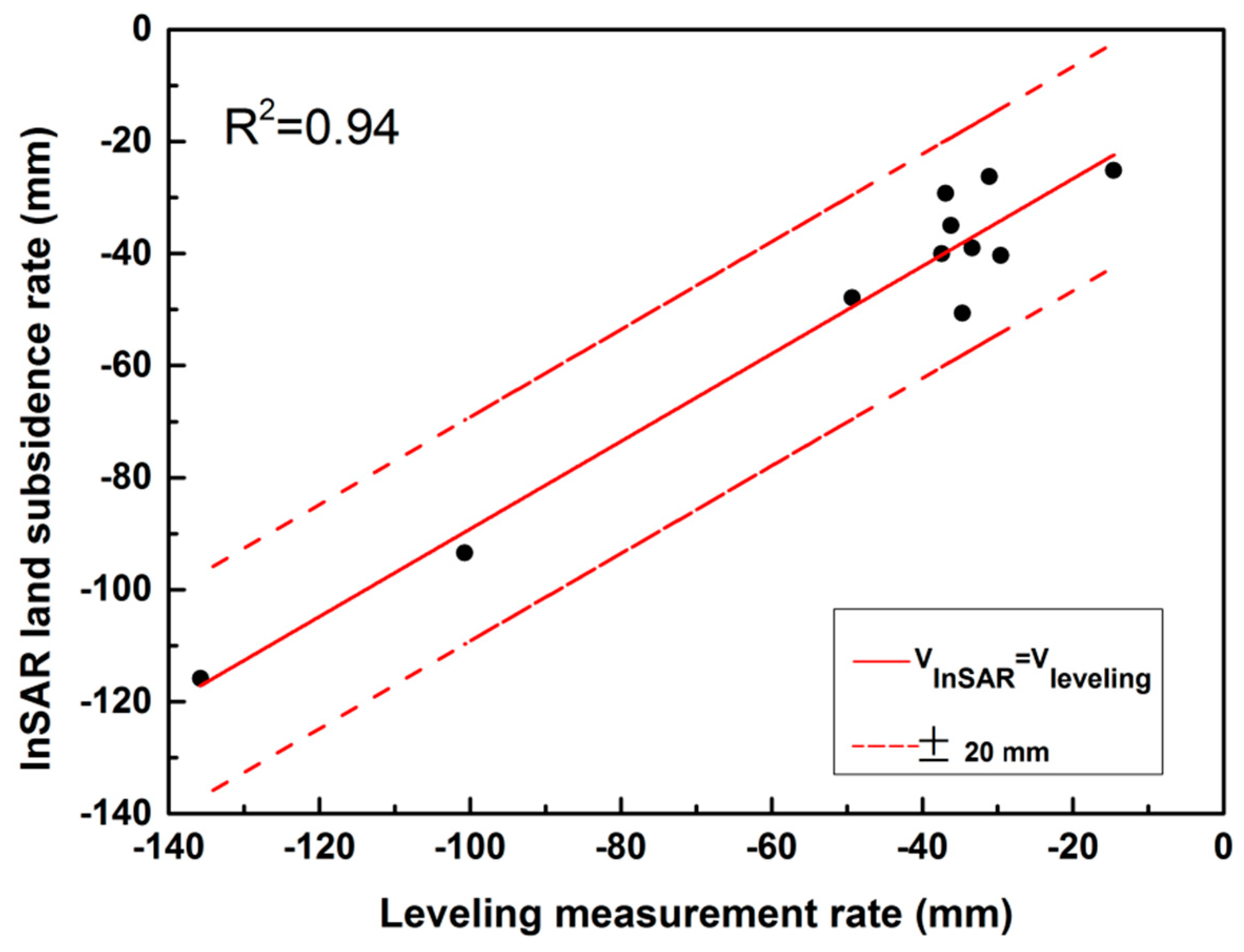
Figure 3.
Cumulative deformation in the study area from 2007 to 2015 measured by the PSI technique using ASAR from 2007 to 2010 and Radarsat-2 data from 2010 to 2015. The red ellipse indicates the standard deviation ellipse (SDE) of the study area. The amethyst cross represents the center of the SDE.
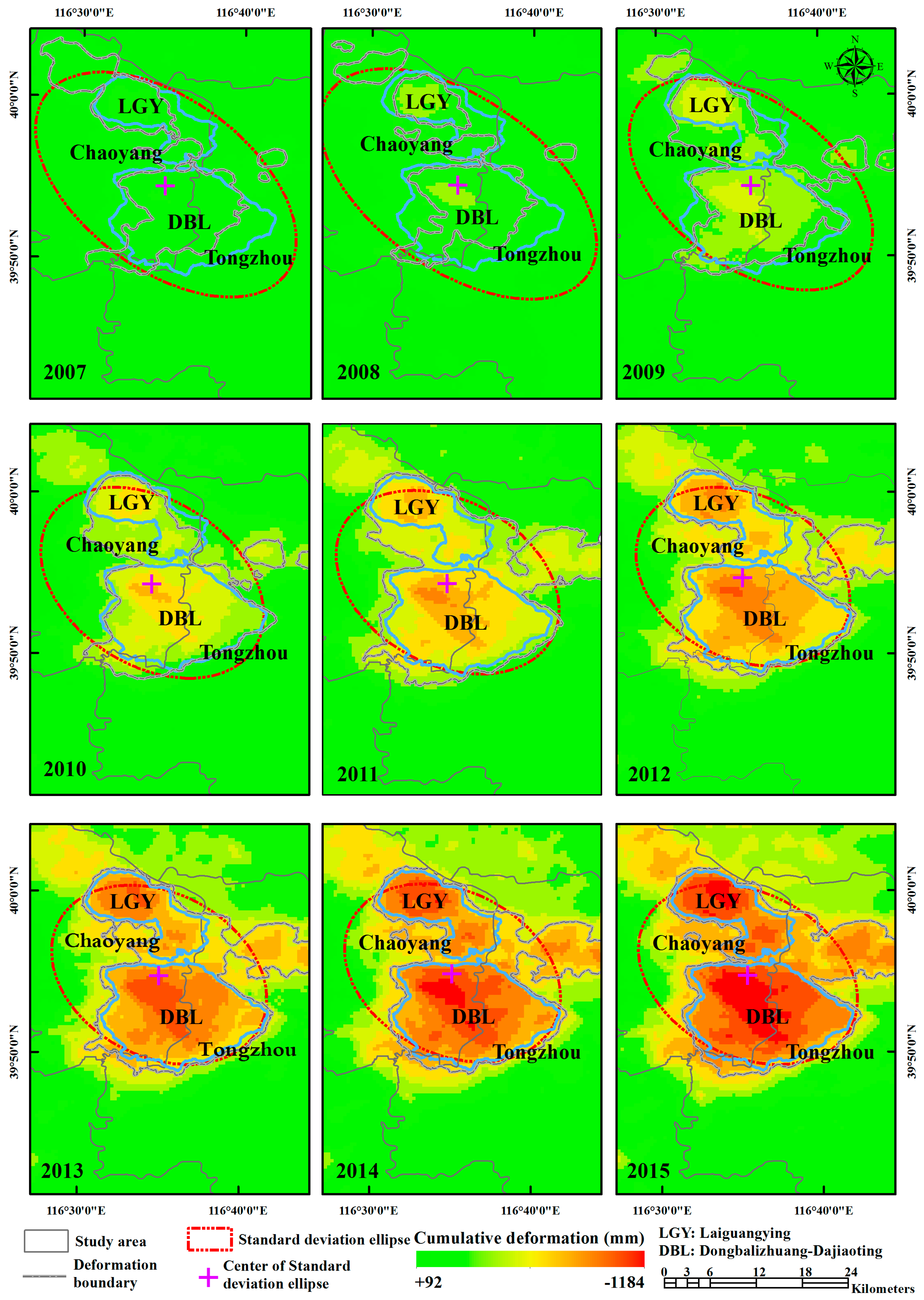
Figure 4.
The area of the land subsidence funnels from 2007 to 2015.

Figure 5.
Changes in the SDE central migration trajectory from 2007 to 2015.

Figure 6.
Temporal changes in the length of the SDE long axis.
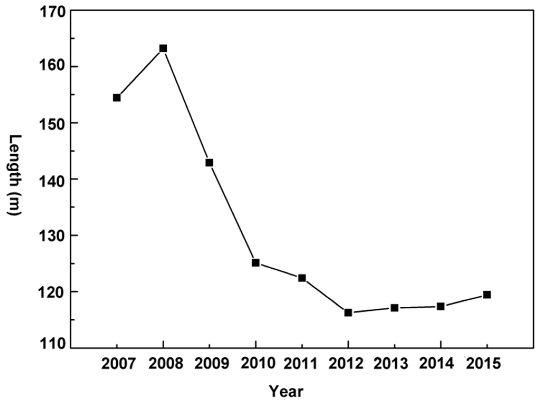
Figure 7.
Changes in the SDE short axis/long axis ratio from 2007 to 2015.

Figure 8.
The PE results for the five wells.The black lines indicate the PE values, and the red lines represent the cumulative land subsidence from 2009 to 2015.
Figure 8.
The PE results for the five wells.The black lines indicate the PE values, and the red lines represent the cumulative land subsidence from 2009 to 2015.

Figure 9.
The spatial evolution patterns of land subsidence obtained by the SDE method. The black countours indicate the changing groundwater level data from 2007 to 2015. The heliotrope lines represent the compressible sediment layer data. The red ellipses indicate the SDEs for every year. In addition, the groundwater level is referenced to sea level.
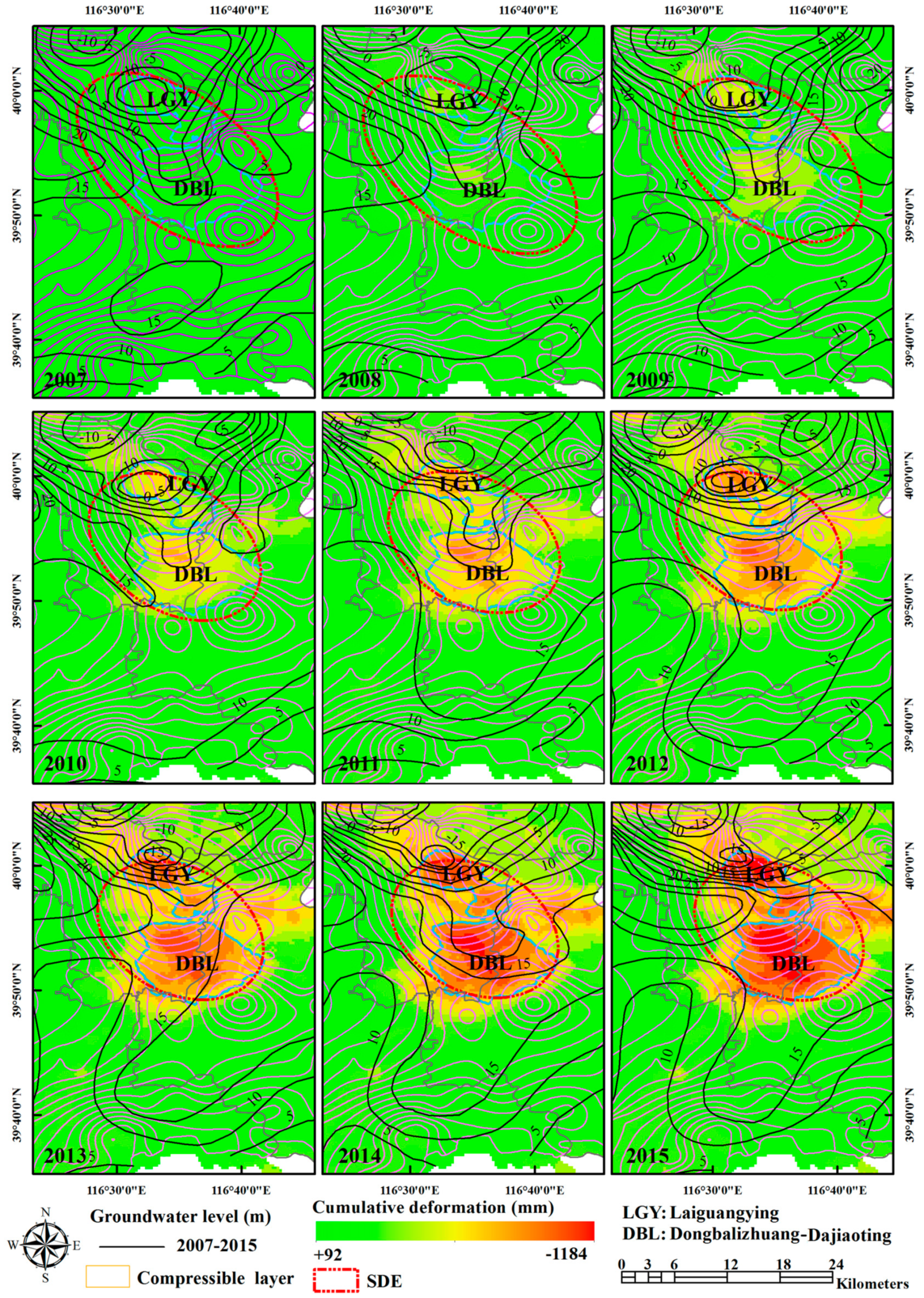
Figure 10.
Comparison of the PE results for well JSL and the variations in the groundwater level. The blue line indicates the groundwater level variations. The black line represents the PE results. In addition, the groundwater level is referenced to sea level.
Figure 10.
Comparison of the PE results for well JSL and the variations in the groundwater level. The blue line indicates the groundwater level variations. The black line represents the PE results. In addition, the groundwater level is referenced to sea level.

Figure 11.
Comparison of the PE results for well BLQ and the variations in the groundwater level. The blue line indicates the groundwater level variations. The black line represents the PE results. The groundwater data reference datum is the same as that in Figure 10.
Figure 11.
Comparison of the PE results for well BLQ and the variations in the groundwater level. The blue line indicates the groundwater level variations. The black line represents the PE results. The groundwater data reference datum is the same as that in Figure 10.

Figure 12.
Comparison of the permutation entropy results for well LHZ and the variations in the groundwater level. The blue line indicates the groundwater level variations. The black line represents the PE results. The groundwater data reference datum is the same as that in Figure 10.
Figure 12.
Comparison of the permutation entropy results for well LHZ and the variations in the groundwater level. The blue line indicates the groundwater level variations. The black line represents the PE results. The groundwater data reference datum is the same as that in Figure 10.


Table 1.
The parameters of the interferometric synthetic aperture radar (In-SAR) data used.
| Parameter. | Envisat ASAR | Radarsat-2 |
|---|---|---|
| Band | C | C |
| Wavelength (cm) | 5.6 | 5.5 |
| Polarization | VV | VV |
| Orbit directions | Descending | Descending |
| Track no. | 2218 | 60115 |
| Incidence angle (°) | 22.9 | 27.6 |
| Heading (°) | −164 | −168.8 |
| Spatial resolution (m) | 30 | 30 |
| No. of images | 31 | 48 |
| Data range | January 2007–August 2010 | October 2010–November 2015 |
© 2019 by the authors. Licensee MDPI, Basel, Switzerland. This article is an open access article distributed under the terms and conditions of the Creative Commons Attribution (CC BY) license (http://creativecommons.org/licenses/by/4.0/).
Share and Cite
MDPI and ACS Style
Zuo, J.; Gong, H.; Chen, B.; Liu, K.; Zhou, C.; Ke, Y. Time-Series Evolution Patterns of Land Subsidence in the Eastern Beijing Plain, China. Remote Sens. 2019, 11, 539. https://doi.org/10.3390/rs11050539
AMA Style
Zuo J, Gong H, Chen B, Liu K, Zhou C, Ke Y. Time-Series Evolution Patterns of Land Subsidence in the Eastern Beijing Plain, China. Remote Sensing. 2019; 11(5):539. https://doi.org/10.3390/rs11050539
Chicago/Turabian StyleZuo, Junjie, Huili Gong, Beibei Chen, Kaisi Liu, Chaofan Zhou, and Yinghai Ke. 2019. "Time-Series Evolution Patterns of Land Subsidence in the Eastern Beijing Plain, China" Remote Sensing 11, no. 5: 539. https://doi.org/10.3390/rs11050539
Note that from the first issue of 2016, this journal uses article numbers instead of page numbers. See further details here.