Machine Learning Approaches for Detecting Tropical Cyclone Formation Using Satellite Data


1
School of Urban and Environmental Engineering, Ulsan National Institute of Science and Technology, Ulsan 44919, Korea
2
Satellite Analysis Division, National Meteorological Satellite Center, Jincheon-gun, Chungcheongbuk-do 27803, Korea
3
Korea Ocean Satellite Center, Korea Institute of Ocean Science and Technology, Busan 49111, Korea
4
Satellite Operation and Application Center, Korea Aerospace Research Institute, Daejeon 34133, Korea
*
Author to whom correspondence should be addressed.
Remote Sens. 2019, 11(10), 1195; https://doi.org/10.3390/rs11101195
Submission received: 15 April 2019
/
Revised: 10 May 2019
/
Accepted: 17 May 2019
/
Published: 20 May 2019
(This article belongs to the Special Issue Advances in Remote Sensing-based Disaster Monitoring and Assessment)
Abstract
:This study compared detection skill for tropical cyclone (TC) formation using models based on three different machine learning (ML) algorithms-decision trees (DT), random forest (RF), and support vector machines (SVM)-and a model based on Linear Discriminant Analysis (LDA). Eight predictors were derived from WindSat satellite measurements of ocean surface wind and precipitation over the western North Pacific for 2005–2009. All of the ML approaches performed better with significantly higher hit rates ranging from 94 to 96% compared with LDA performance (~77%), although false alarm rate by MLs is slightly higher (21–28%) than that by LDA (~13%). Besides, MLs could detect TC formation at the time as early as 26–30 h before the first time diagnosed as tropical depression by the JTWC best track, which was also 5 to 9 h earlier than that by LDA. The skill differences across MLs were relatively smaller than difference between MLs and LDA. Large yearly variation in forecast lead time was common in all models due to the limitation in sampling from orbiting satellite. This study highlights that ML approaches provide an improved skill for detecting TC formation compared with conventional linear approaches.
1. Introduction
A tropical cyclone (TC) can lead to tremendous economic losses and casualties when it makes a landfall [1,2]. Since any tropical disturbance with a sufficient magnitude has a potential to be developed abruptly into a TC over the warm ocean, it is highly desirable to have an accurate forecast system for TC formation for a timely warning to the public. There are several approaches to predict TC formation. One is to use numerical weather prediction (NWP) models, which has been significantly improved in the past years due to the advance in modeling techniques and physics parameterizations, more available satellite data for the better initialization, and enhanced computing resource. For example, Halperin et al. [3] investigated the forecast skill for TC genesis in the North Atlantic from 2004 to 2011 by five NWP models, and showed that their conditional probability of hit ranged from 26% to 44%. Nevertheless, it still remains challenging for most NWP models to predict whether a tropical disturbance will develop to a TC or just decay as a non-developer [4,5].
An alternative is to use various types of statistical models that have been developed to predict the TC formation based on large-scale meteorological conditions identified as important processes for TC formation. Schumacher et al. [6] produced an estimation of 24-h probability of TC formation in each sub-region of various ocean basins. They combined large-scale environmental parameters derived from the National Center for Environmental Prediction (NCEP)-National Center for Atmospheric Research (NCAR) reanalysis [7], and multiple geostationary satellites. Similarly, Hennon and Hobgood [8] considered eight large-scale predictors such as latitude, daily genesis potential, maximum potential intensity, moisture divergence, precipitable water, pressure tendency, surface vorticity tendency, and 700-hPa vorticity tendency from 6-hourly global NCEP-NCAR reanalysis [7]. The foregoing studies [6,8] commonly used a Linear Discriminant Analysis (LDA) classifier in the prediction of TC formation. Fan [9] applied a multi-linear regression method from large-scale environmental factors based on NCEP-NCAR reanalysis data for detecting the Atlantic TC formation.
While the above-mentioned statistical methods require a linear statistical relationship between predictors (e.g., large-scale environmental parameters) and predictand variables (e.g., tropical cyclone formation possibility), TC formation involves complicated multi-scale interactions from large-scale environmental to mesoscale convective processes [10]. Hennon et al. [11] pointed out limitations in the use of the LDA or linear regression approaches due to the assumption of the linear relationship between predictors and predictands. On the other hand, machine learning (ML) approaches do not require any assumption in contrast to the conventional statistical techniques based on linear models [12]. There are several ML approaches widely used such as decision trees (DT), random forest (RF), and support vector machines (SVM). While DT is a simple classifier that recursively partitions data into subsets based on tree-like decision rules, RF uses a bootstrapping method to make an ensemble of classification trees [13]. SVM, which is a non-parametric statistical learning technique, builds a hyperplane to separate the dataset into a discrete, predefined number of classes. The hyperplane is adjusted for minimizing misclassifications during a training procedure [14]. Very recently, the ML approach has been applied to the model for classifying TC formation [15,16]. Zhang et al. [16] utilized DT to classify developing and non-developing tropical disturbances using several predictors (e.g., maximum 800-hPa relative vorticity, sea surface temperature, precipitation rate, vertically averaged divergence, and air temperature at 300 hPa) derived from the Navy Operational Global Atmospheric Prediction System analysis data [17]. They showed that the accuracy in the forecast of TC formation prior to 24 h was about 84.6%. Park et al. [15] also applied the DT technique for detecting TC formation. They trained DT rules using system-representative parameters such as the symmetry of low-level circulation pattern, intensity, and the organization indices that derived from the sea surface wind data from WindSat [18].
The dependency of ML approaches has been tested in various remote sensing applications. For example, Han et al. [19] developed a convective initiation algorithm from the Communication, Ocean, and Meteorological Satellite Meteorological Imager [20] based on the three ML approaches—DT, RF, and SVM. Their results showed that RF produced a slightly higher hit rate (HR) than DT with a comparable false alarm rate (FAR), while SVM resulted in relatively poor performance with much higher FAR compared with the other two techniques. On the other hand, Sesnie et al. [21] compared SVM with RF to classify 11 Costa Rican tropical rainforest type using the Landsat thematic mapper bands and the normalized difference vegetation index, where they found that SVM performed better with higher accuracy than RF. This suggests that there is no single best ML technique applicable to all cases, and the performance of the ML algorithm depends not only on the technique but also on the type of application and input data.
This study is an extension from the study of Park et al. [15]. Although it demonstrated a skill level practically useful in detecting TC formation, it was limited by using a single ML algorithm (i.e., DT) and could not evaluate the room for further improvement when the other algorithms were tested. In this study, three ML approaches have been tested to examine the dependence on the technique. An identical dataset of predictors is applied to the ML algorithms and calibrated independently, and then validated for comparing the detection skill. In addition, the performance is also compared with that by LDA with a quantitative skill assessment. TC formation processes are complicatedly involved with instability in the atmospheric and oceanic dynamics and thermodynamic processes that are not necessarily linear [22]. This study hypothesizes that ML, which can account for nonlinear relationships among the predictors [23,24], should be more suitable than LDA for the application to tropical cyclogenesis forecast.
2. Data and Methods
2.1. Data and Preprocessing
To characterize tropical disturbances at their formation stage of TC, this study used all-weather wind speed and direction at 10 meter above the ocean surface and rain rate measured by the WindSat polarimetric microwave radiometer (http://www.remss.com/missions/windsat) onboard the Department of Defense Coriolis satellite developed by the Naval Research Laboratory, the Naval Center for Space Technology for the U.S. Navy, and the National Polar-orbiting Operational Environmental Satellite System (NPOESS) Integrated Program Office (IPO). The satellite was launched on 6 January 2003 and has been operating in the present time. Ocean surface wind vector product covers a wide area with an average swath width of 950 km. Retrieving ocean surface wind signal under rainy conditions has been a long-standing challenge for passive microwave radiometers due to the contamination by rain. The WindSat radiometer uses fully-polarimetric channels at 10.7, 18.7, and 37.0 GHz and dual-polarimetric channels at 6.8, and 23.8 GHz. Using multiple channels, particularly C-band (4 to 8 GHz) and X-band (8 to 12 GHz) where the atmospheric attenuation is relatively small, allows developing an algorithm for retrieving wind speed in hurricanes even under heavy rain to a reasonable degree of accuracy. The wind speed retrieval accuracy for tropical cyclones ranges from 2.0 m s−1 in light rain to 4.0 m s−1 in heavy rain. It also shows no degradation of wind speed signal at wind speeds up to 35 m s−1, well above the magnitude of the tropical depression. The liquid water precipitation is derived by using 18.7, 23.8, and 37.0 GHz channels. The horizontal resolution of the WindSat measurement is for 6.8 GHz, for 10.7 GHz, for 18.7 GHz, km for 23.8 GHz, and for 37.0 GHz, respectively. The dataset has been re-processed to gridded data for the current analysis.
This study uses 1,325 WindSat overpass images including approximately 630 tropical disturbances in the western North Pacific during the years of 2005-2009. The satellite observations are collocated with the system track data from the Joint Typhoon Warning Center (JTWC) best track, and Tropical Cloud Cluster [25]. A tropical disturbance is classified as a developing (DEV) disturbance when the maximum sustained wind (MSW) speed will be larger than 13 m s−1 later to be denoted as a tropical depression (TD) (announced by JTWC). In addition, the image needs to cover sufficiently large area near the center of disturbance (at least 60% of non-missing data within 4-degree radius of circle) at least once before TD stage and the data need to be sampled again no later than 72 h after TD stage. The remaining disturbances are defined as non-developing disturbances (non-DEV). In the case of non-DEV disturbance, all available satellite observations are collected.
Park et al. [15] used eight specific predictors that quantitatively describe dynamic and hydrological characteristics related to TC formation, and determine either DEVs or non-DEVs based on the DT-based rules. This study uses the same predictors, and a brief description of them is given here. Two indices, “wind_ave” and “rain_ave”, are aimed to represent the intensity of low-level wind and rain rate near the tropical disturbance center, respectively. To quantify the degree of symmetry in the low-level circulation for developing cyclones, two indices are designed by calculating circular variance (CV), “wind_cv_fix” and “wind_cv_mv”, in which the former calculated CV over a full domain ( Lat./Lon.) centered at the target disturbance for characterizing synoptic-scale circulation, and the latter over a smaller subdomain ( Lat./Lon.) moving around the disturbance for characterizing mesoscale circulation. The remaining four indices include “wind_ci”, “wind_pladj”, “rain_ci”, and “rain_pladj”, which represent the clumpiness index (CI) and the percentage of like adjacencies (PLADJ) for wind and rain rate, respectively. These two measures are defined from Fragstats statistics [26]. Both PLADJ and CI quantify the degree of organization of strong wind and heavy rainfall areas. Table 1 summarizes the eight predictors used in this study.
2.2. Sampling
Training a prediction model should not be significantly influenced by insufficient samples. To examine the sample dependence, this study performed the k-fold cross validation, where all available WindSat data archived for five years were divided into the training and the validating sub-datasets [27]. Verification of the model fitted with different samples can help estimate the uncertainty and the sample dependence of the statistical model in a quantitative manner as well as evaluate the year-to-year variability of the prediction skill. Three-year data randomly selected out of five years were used for training, and the remaining two-year data were used for validation. This resulted in 10 different training-validation datasets to be tested. In the original dataset, the number of non-DEV was about three times larger than that of DEV. As the training with the ML approaches such as DT using unequal samples between DEV and non-DEV may cause a bias in the model [28], non-DEVs were resampled randomly as much as DEVs for training. Resampling was repeated for 100 times for each 10 different k-folding datasets, leading to 1000 datasets total for model development and validation for each TC formation detection model.
2.3. Model Construction
2.3.1. Linear Discriminant Analysis (LDA)
LDA has been widely used in a variety of classification studies [7,29,30]. LDA is a statistical technique to classify objects into two groups based on a set of predictors with specific threshold values. LDA projection has a known caveat that the classification ability is decreasing for the non-linear relationship between predictors and the predictand [31]. To construct a model based on LDA, multiple regression models were performed in this study given the eight potential predictors. The predictors were tested following procedures to avoid overfitting problems. All the possible combinations of predictors were tested in terms of the validating statistics using HR, FAR, and Peirce Skill Score [32] (hereafter referred to as PSS) and then the predictors of less significance were eliminated one by one.
2.3.2. Decision Trees (DT)
DT has been introduced in many recent remote sensing studies for both classification and regression [15,33,34,35,36,37], in which the data sample is subject to the partitioning into subdivisions repeatedly based on decision rules, resembling branches in a tree [38]. The advantage of the DT is to enable easy interpretation and physical insights to the classification rules as it provides visible if-then rules with the relative importance of predictors. This study used the C5.0 program developed by RuleQuest Research, Inc [39]. Unlike the LDA, DT (the other two ML approaches as well) selects an optimal combination of predictors empirically by itself through training. To evaluate the degree of fitting for 1000 different training datasets, overall accuracy is calculated which represents the ratio of samples correctly classified.
2.3.3. Random Forests (RF)
RF is an ensemble approach based on classification and regression trees (CART), which was originally designed to improve the well-known problem of DT that is sensitive to training data configuration [40]. RF has been widely used in remote sensing applications for both classification and regression tasks [41,42,43,44]. RF adopts two randomization processes to develop numerous independent decision trees and the final decision is made by majority voting (or weighted voting) strategy [19,45]. RF also provides the relative importance of a specific variable, as represented quantitatively by the mean decrease of accuracy when the variable is permuted to random values. The critical predictor has a higher variable importance than others. This study used the R software [46] to fit the data into the RF algorithm.
As the RF model contains a random process in the training, each round of training was likely to produce no identical result even with the same data. Each set of training dataset were repeated five times to produce the RF model for obtaining reliable results.
2.3.4. Support Vector Machines (SVM)
SVM is one of the widely-used machine learning models in remote sensing applications in recent years [47,48,49,50,51], which finds an optimal hyperplane to classify data [52]. SVM utilizes a kernel function to transform the data dimension into a higher one in order to identify an optimal hyperplane effectively [53]. Among the linear, polynomial, and radial basis functions, the radial basis function was turned out to be the best as a kernel function in our test. The kernel and penalty parameters used in the SVM model were automatically adjusted during the data training process to ensure the best performance in detecting tropical cyclone formation. Before data training, each predictor variable was linearly scaled to the range from 0 to 1 in order to consider the difference in magnitude across the variables. This procedure also helps reduce computational time in optimizing SVM model parameters. Compared with other machine learning algorithms, SVM does not provide the information on the relative importance of predictors instantaneously. As an alternative, the F-score test is applied to identify the major discriminating features that characterize the tropical cyclone formation based on the SVM method. The F score, also called the F1 score or F measure, is a measure of a test’s accuracy, which is defined as the weighted harmonic mean of the test’s precision and recall [54]. From the contingency table of observed versus the model-classified number of DEVs and non-DEVs, precision is the number of correct DEV forecasts divided by all forecast DEVs, and recall is the correct DEV forecasts divided by all observed DEVs. The SVM model can make different results according to the kernel optimization procedure. Each sample was repeatedly trained five times to produce reliable output from the SVM model. This study used the library for the SVM software package, LIBSVM [55] version 3.22 available at http://www.csie.ntu.edu.tw/~cjlin/libsvm.
2.4. Verification Methods
The performance of the trained models is compared using HR, FAR, and PSS from the contingency table of observed versus the model-classified number of DEVs and non-DEVs. HR is the number of model-classified DEVs divided by the number of observed DEVs. FAR is defined as the number of the model-classified DEVs divided by the number of observed non-DEVs. The PSS score [32] is based on the proportion correct as the basic accuracy measure and it is defined as the relative improvement over the reference forecast. The perfect score receives PSS =1, forecasts equivalent to the reference forecast receive zero scores, and forecasts worse than the reference forecasts receive negative scores. The reference accuracy measure is the proportion correct that would be achieved by unbiased random forecasts. It can be easily shown that the PSS is simply the difference between HR and FAR, and it provides a combined measure of the forecast skill. The detection lead time by model for each observed DEV was calculated, which was defined as a time difference between the first TC formation detection and the time when it actually developed to TD according to the JTWC best track. Negative (positive) lead time means that the model detection is made before (after) the actual TC formation.
3. Results
3.1. Model Calibration
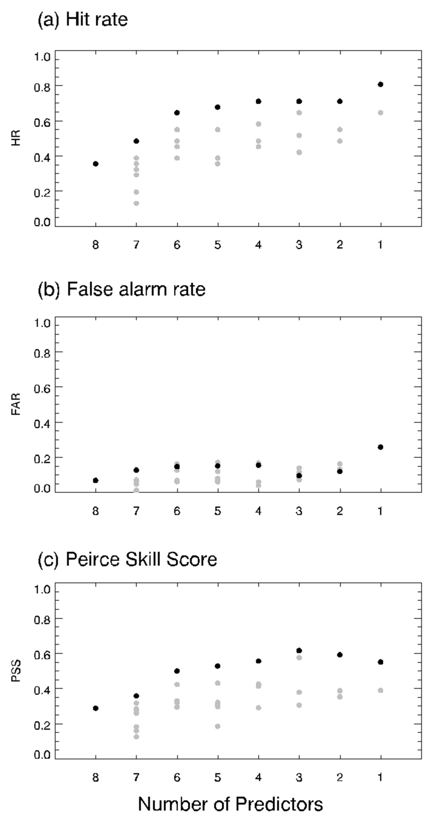
Using eight predictors with the 1000 datasets, each TC formation model was trained independently using LDA and the three ML approaches. In calibrating the LDA model, all the possible combinations of potential predictors were tested in advance. Figure 1 compares the performance for various combinations of predictors and the number of predictors. HR increases significantly by reducing the number of predictors (Figure 1a). By contrast, FAR increased gradually in general. However, the lowest (best) values were found when the number of input predictors is 3 or 4 (Figure 1b). As seen in Figure 1c, PSS results indicated that the number of three predictors with the use of wind_ave, wind_cv_fix, and wind_pladj showed the best performance among the all other sets. Table 2 shows the average and standard deviation of coefficients for each predictor after applying the model for 1000 different training datasets. This model in Table 2 was applied to the validation dataset.
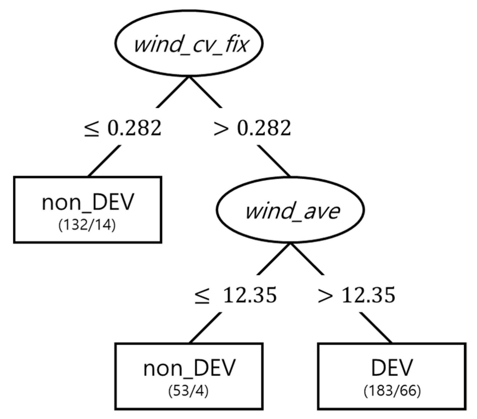
The training results for 1000 different training datasets for the DT model showed the accuracy (i.e., the ratio of samples correctly classified) ranging from 72.9% to 91.1%. In each training, DT selected a different set of predictors. Nevertheless, the wind_cv_fix was included in all tests and wind_ave was included 83% of the tests. On the other hand, rain_ave and rain_ci were selected least as 33% and 30%, respectively. Although the major advantage of DT is to display its rules, each algorithm contains different combination of predictors and thresholds. Figure 2 shows an example that consists of three if-then decision rules used for binary classification of tropical disturbances into DEV or non-DEV. This case selected only two variables of wind_cv_fix, and wind_ave. As mentioned, these are the most frequent variables in the DT training process and they were also used in Park et al. [15].
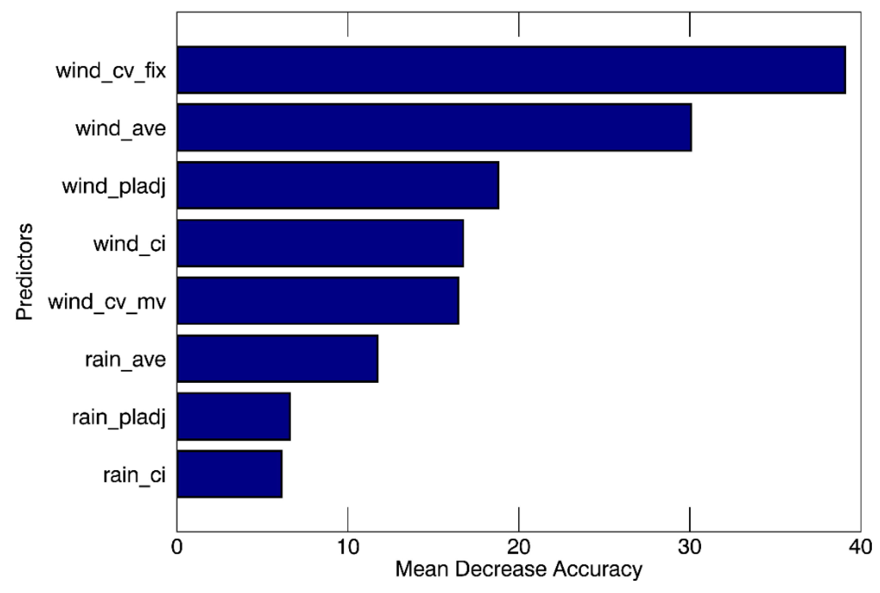
In developing a RF model with eight predictors, Figure 3 showed the mean decrease accuracy for each predictor obtained from training with 1000 sample datasets. The predictors of wind_cv_fix and wind_ave were revealed to be most important with the mean decrease of the accuracy of 38.60 and 30.19, respectively. The accuracy of RF was 100% for all tested sample datasets. This is common in the calibration stage for RF as it consists of not-pruned decision trees [40].
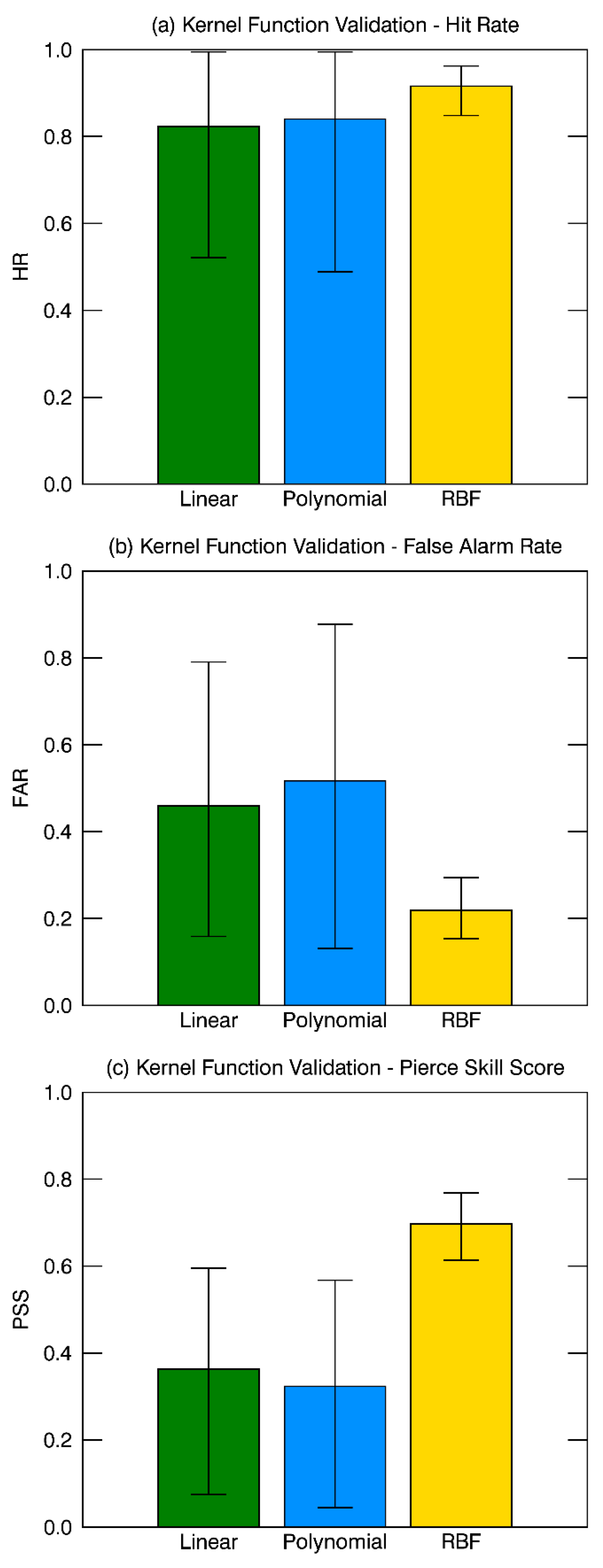
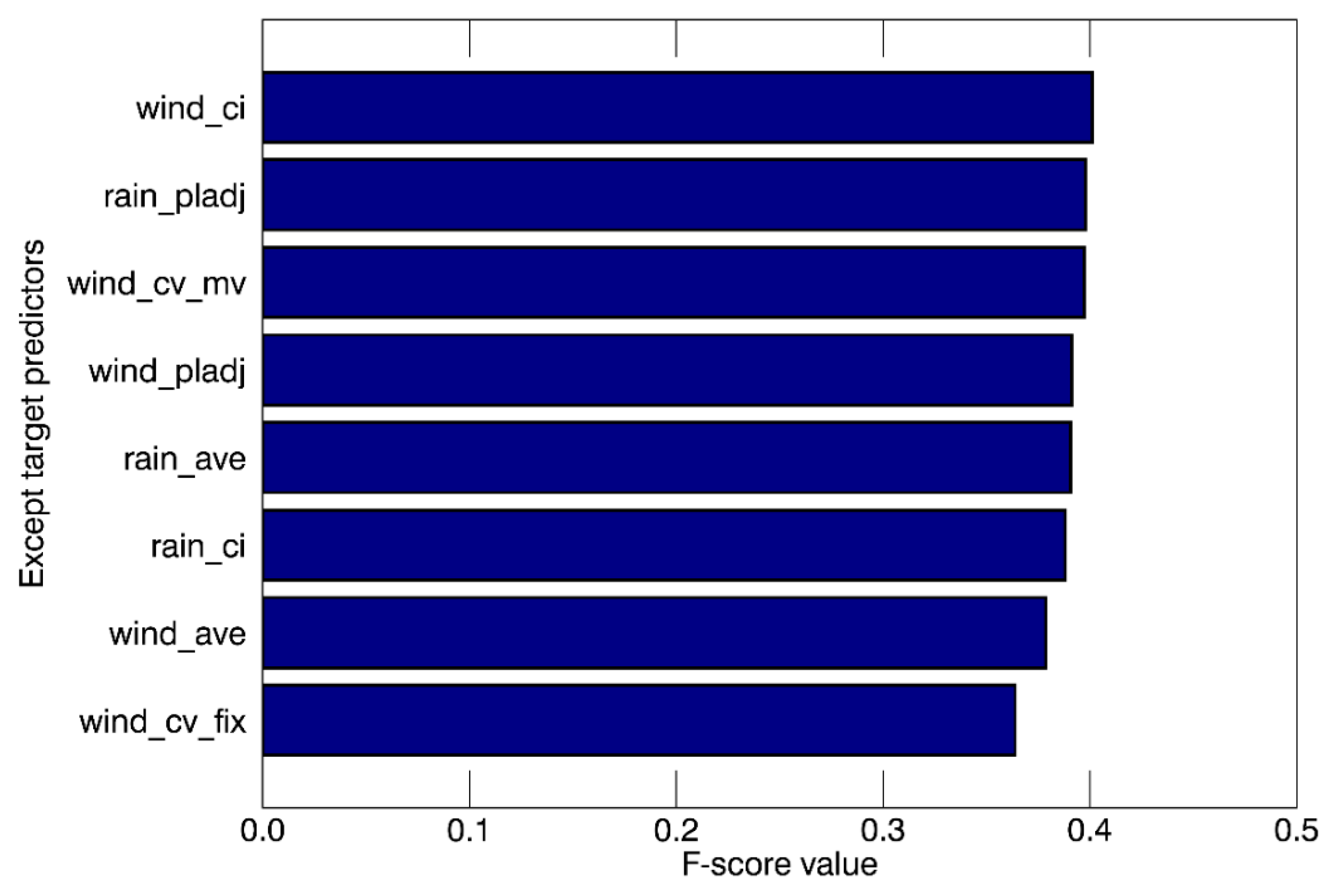
As mentioned in the model construction part, three different types of kernel functions were tested to figure out the best (Figure 4). In the case of HR, the radial basis function kernel showed much higher HR (91.6%) than the other two kernels, with the lowest FAR (22.0%). As a result, it showed the best performance based on PSS. Figure 5 shows F-score values from the SVM training results using the radial basis function. Each F-score value was measured using seven predictors without denoted target predictor so that a lower value of F-score indicates lower classification ability when the specific predictor is excluded. As a result, wind_cv_fix and wind_ave were identified as the most important predictors in detecting tropical cyclone formation which was consistent with the cases of other machine learning models.
3.2. Verification
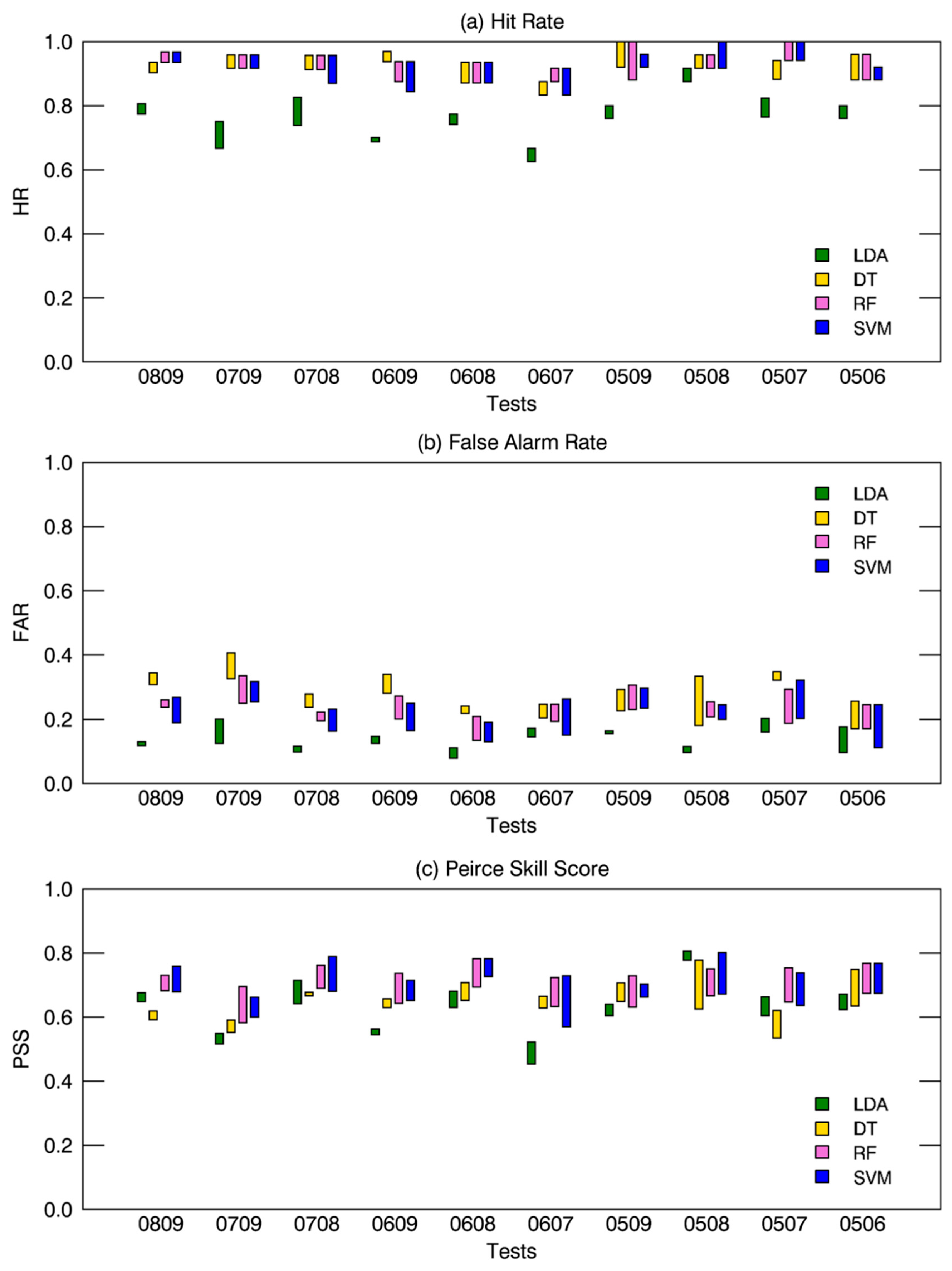
Figure 6 compared the performance skill for LDA and the three ML approaches from all cases of validation (i.e., 1000 cases), in terms of HR, FAR, and PSS. Figure 6a is the comparison of HR for the four different models, in which the total averaged HR of three ML approaches (94%) is consistently higher HR than that from LDA (77%). The ML approaches produced relatively smaller HR variation due to the different sample years compared with that in the LDA (16%), suggesting that LDA had larger discrepancies along with the validation period. A few cases in ML approaches could hit TC genesis perfectly (e.g., 0509 in DT and RF, 0507 in RF, and 0508 in SVM).
As shown in Figure 6b, LDA (13%) showed lower FAR than ML approaches, although a few cases showed comparable values (e.g., 0506 in Figure 6b). The FAR in LDA changes relatively little with 1–11% variation using different validating data samples, while that in ML approaches vary more with 2–23% variation. FAR changes more at the change of validation samples, about 10% in LDA and 10–17% in ML approaches, respectively. This result indicated that LDA could classify DEV and non-DEV with small variances and little affected by the validating samples. There was a small difference among ML approaches in the case of HR, but in contrast, FAR showed a large variation among ML approaches. DT (28%) had the largest FAR compared with RF (23%) and SVM (21%).
In the case of HR, ML approaches had relatively higher performance than LDA, on the other hand, LDA showed much lower FAR than ML approaches. To consider both HR and FAR simultaneously, PSS was introduced in Figure 6c. The PSS, as mentioned above, estimated the goodness of a classifier in the binary classification. The overall results showed that ML approaches, in general, had higher PSS than LDA. Differences depending on the validation samples showed that ML approaches (10–17%) produced less variation than LDA (20%), which is consistent with the case of model calibration results (Section 3.1) exhibiting 7–17% variation for ML approaches and 18–29% for LDA. In the case of RF and SVM, they gave a higher classifying ability between DEV and non-DEV. However, DT had comparable skills with LDA.
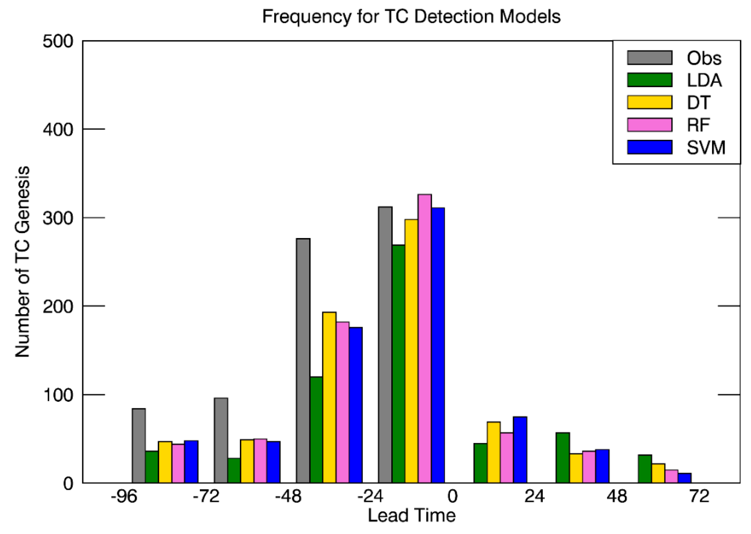
To assess a prediction ability of each model, Figure 7 shows histograms of the lead time classified as TC by LDA (green), DT (yellow), RF (pink), and SVM (blue), and of the first time the WindSat is available (gray). In this figure, zero lead time represents the first time to reach an intensity of TD according to the JTWC best track, and early detection of TC has negative (positive) lead time which located left (right) relative to zero lead time. The frequency of the first observation from WindSat showed the maximum between 0 and −24 h, and radically decreased in the early time before −72 h. A smaller observation number from WindSat in earlier developing stage was in part due to the fact that the disturbance tracking backward in the time needed to be stopped in the premature or less-organized stage of disturbances. The frequency of the first detected time by the WindSat observation (gray) and that by the LDA and ML models showed a similar distribution. Although all models were able to predict TC formation when the WindSat observation was available in advance, the result demonstrated that ML approaches were able to detect TC formation earlier than LDA (Figure 7).
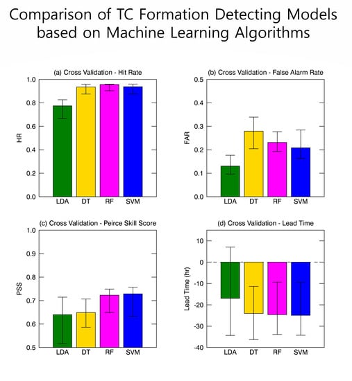
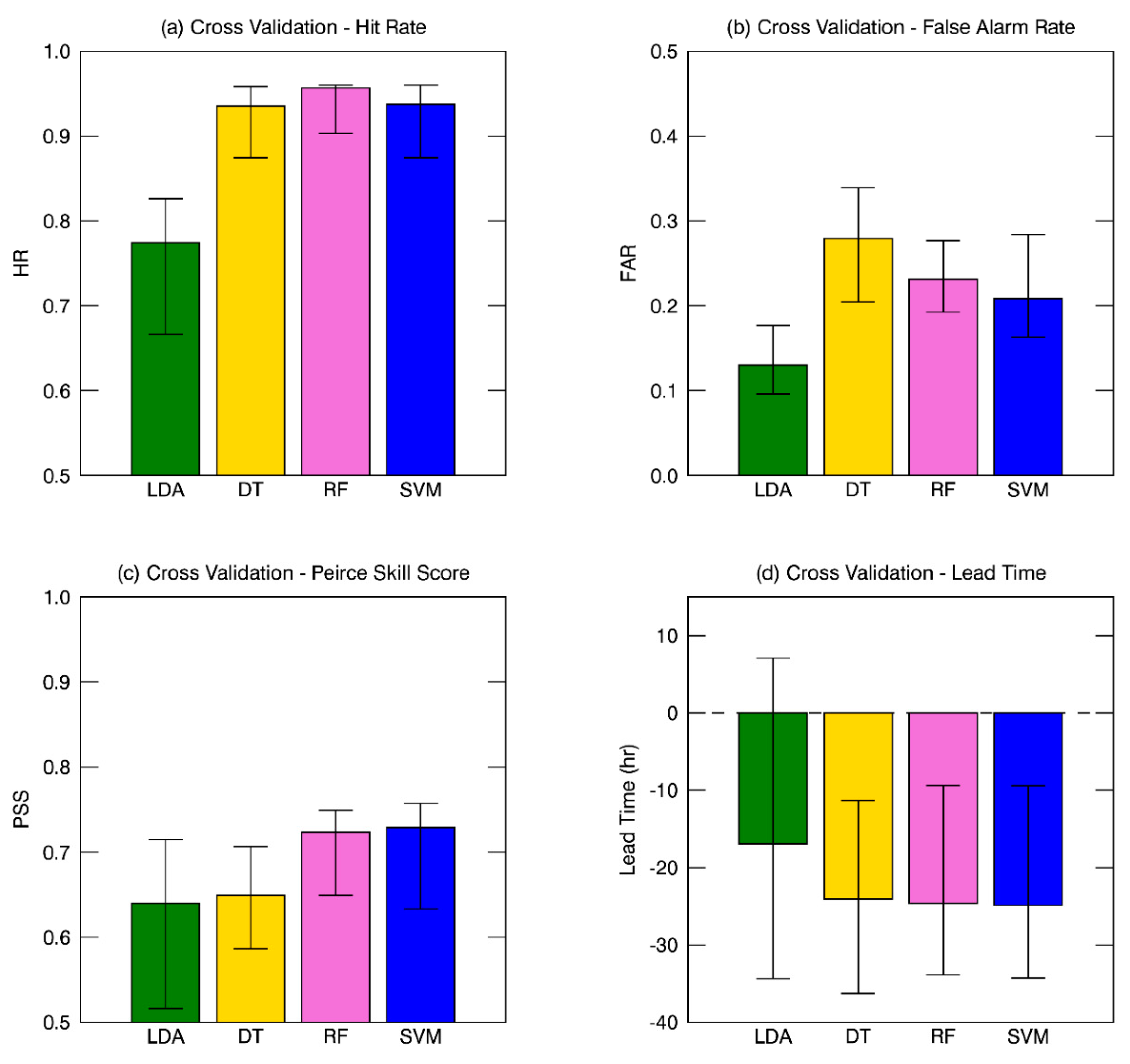
Figure 8 summarized the results of four different TC formation detecting models in terms of HR, FAR, PSS, and lead time. Each box plot represented median values among 1000 tests and upper and lower boundaries represented 90 and 10 percentiles, respectively. Median HR showed that ML approaches (0.94–0.96) outperformed LDA (0.77). RF had the lowest (0.09) and LDA had the highest (0.25) error boundary. Figure 8b showed that LDA (0.13) had a better FAR than ML approaches (0.21–0.28) although they occasionally had the similar ability (e.g., 0506 in Figure 7b). Among the ML approaches, they showed different FAR and variances. In particular, DT tends to have more missed cases (28%) than RF (23%) and SVM (21%). The PSS results may be divided into two groups according to their skill score. The RF (72%) and SVM (73%) showed relatively higher score than DT (65%) and LDA (64%). The PSS is directly connected with HR and FAR in that is calculated by the difference between HR and FAR. Two high PSS models had a high HR with low FAR, however, the two lower models had different reasons that DT had the highest FAR although it had high HR and LDA had the lowest FAR with lower HR (Figure 8). Nevertheless, DT had a lower variance of validating results rather than LDA. In the case of lead time in Figure 8d, even though the same satellite observations are given, ML approaches (26–30 h earlier) could have earlier detection of TC genesis than LDA (21 h earlier). All models showed a large difference in lead time due to the infrequent WindSat sample. LDA sometimes showed after detecting cases (positive lead time).
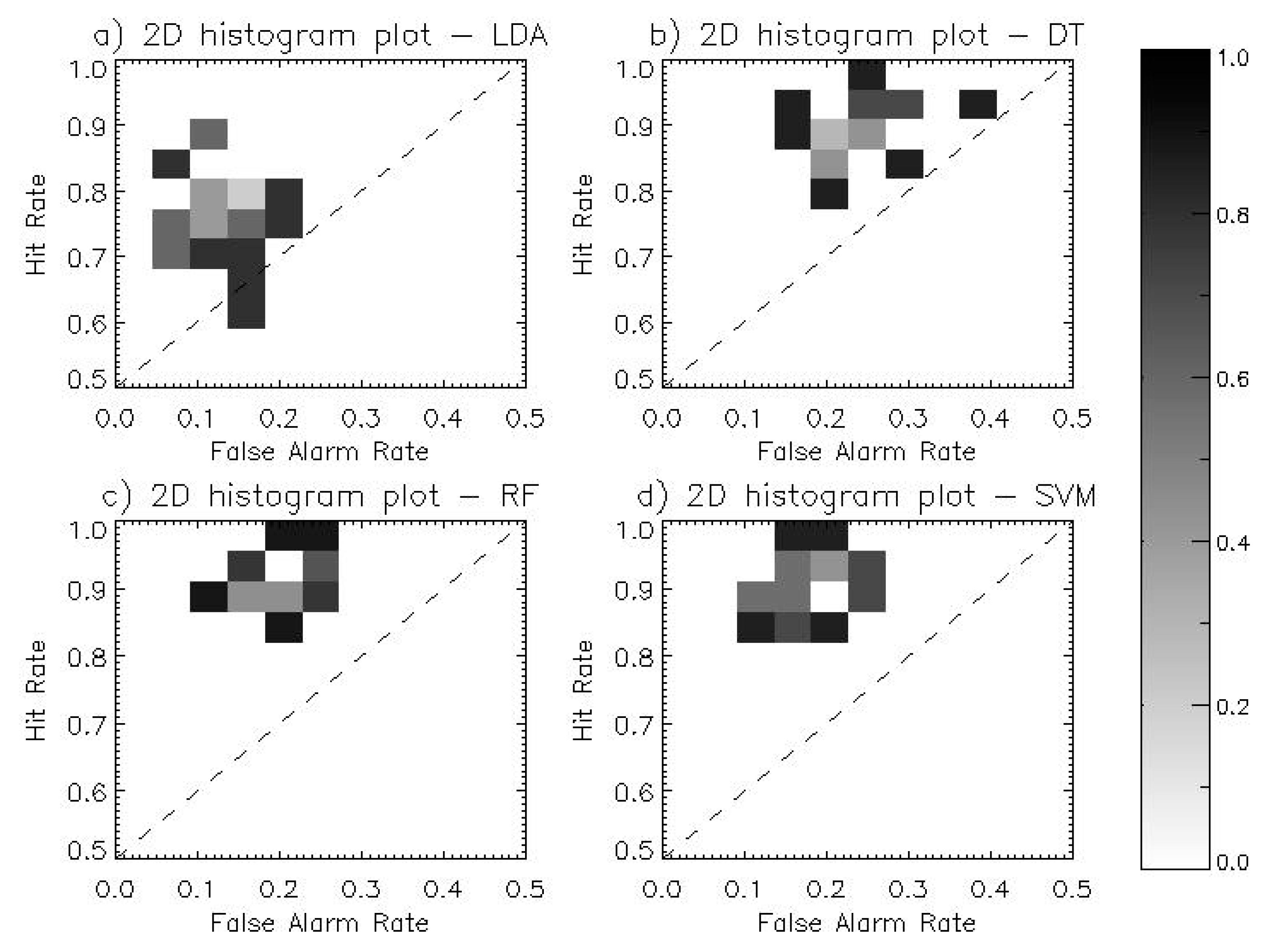
As alternative ways to compare the performance of four TC genesis detection models, two-dimensional histogram plot was made with FAR (x-axis) and HR (y-axis), which results were given in Figure 9. A skillful model that achieves much higher HR and less FAR, so that it tends to be located on the top left corner of the plot. A model which has no skill, on the other hand, lies along or under the diagonal (i.e. the model has no skill better than arbitrary choice). Each distribution from the three ML approaches (Figure 9b–d) was clearly separated from that of LDA (Figure 9a). The ML approaches had the advantage of better HR, whereas LDA tended to have smaller FAR. It was also noted that RF and SVM were located more to the left than DT, ensuring better performance in terms of FAR. Because RF was made for complementing the defect of DT, RF outperformed DT in general. It is possible that training procedures are affected by the lack of samples and quality even though applying random sampling methodology. There are many studies suggesting that SVM performs better with small samples [48,56,57,58], which is consistent with the results of this study.
4. Discussions
The formation of TC involves various dynamical and physical processes in multiple spatial and time scales [5,10]. Previous regression-based models [6] may not be appropriate to deal with complicated nonlinearities involved in the TC formation process. This study suggested an alternative approach for calibrating such an intricate formation process based on the ML approaches. The HR by ML approaches tested in this study was similar to values ranging from 94% to 96%, which were in general higher than that by LDA. Despite the ML approaches showed a higher FAR ranging 21–28% than that by LDA (~13%), they outperformed in the classification skill measured by PSS. The ML approaches also demonstrated a useful skill in the detection time, which was 26–30 h earlier than actual TC formation. The detection time by MLs was even earlier by 5–9 h compared with that by LDA.
The detection performance of the models developed from this study can be compared with those from existing studies, although an exact comparison may not be possible due to the differences in data and methods. The average hit rate of 95% by ML adopted in this study is obviously higher than that of numerical TC forecast models. Multi-model numerical weather forecasts were reported to show an average of 20% of the conditional probability of hit over the period of 2007–2011 [3], although they were tested with more strict criteria for the detection of tropical cyclones such as the more limited allowance of detection time and the genesis location. The results also exhibited a large dependence on the numerical models tested. By and large the statistical models such as ones used in this study show a more consistent and reliable performance than the numerical models. In our study, RF and SVM showed comparable skills, although SVM slightly underpredicted the tropical cyclone formation.
Our results can be compared with the skills from other ML approaches. The DT model in this study performed 93.5% of HR and 27.9% of FAR, while those from Park et al. [15] showed 95.3% and 28.5%, respectively. Although both studies used the identical DT algorithm, the previous study tested with fewer samples compared with the current study. The overall accuracy of classification by Zhang et al. [16] using DT was 84.6%, which was slightly lower than that from this study (~95%). The skill difference seemed to be partly related to the difference in the number of samples, where Zhang et al. [16] used approximately 2000 samples while this study used 1000 samples or more. The lead time for detecting TC formation by DT was 26 h in this study, which was comparable to that by Zhang et al. [16] with 24 h. Another reason for skill difference seemed to be related with the selection of predictors, where Zhang et al. [16] used large-scale environmental predictors derived from global atmospheric reanalysis and SST while this study used the direct information for disturbances in terms of their surface wind and rain rate.
Due to the complexity of RF- and SVM-based algorithms, they are difficult to visualize in terms of decision rules in detail. One can examine the relative importance of each input variable, instead, to identify the important dynamical or physical characteristics in the TC formation. DT and RF commonly revealed that the wind intensity average (wind_ave) and the degree of symmetry (wind_cv_fix) in the ocean-surface wind pattern near the disturbance center were the most critical predictors, even though their training procedures were independent. In the LDA model, the linear equation was composed with the degree of the strong wind organization (wind_pladj) in addition to the foregoing two variables.
The lead time how early the model can predict the TC formation depends strongly on the time of data availability. This study used the polar-orbiting satellite observations which were often missing or too late for detecting the formation potential. There are at least two ways for further advancing TC genesis prediction time such as 1) to advance the first observation time over a disturbance by utilizing other sources of ocean surface wind measurements such as the ASCAT [59] and 2) to advance the first time by developing an algorithm using a geostationary satellite for continuous monitoring of tropical disturbances.
The comparison among the three ML approaches revealed a slight difference in the performance. SVM exhibited less FAR compared with the other ML approaches, although all showed comparable skill in terms of HR. The results are consistent with previous studies [19,36] in different application also showed that RF performed better than DT. However, it is admitted that our result is still preliminary in terms of limited sample datasets from satellite. More extensive studies are required for the performance comparison between ML approaches, once more data are available in the near future.
5. Conclusions
This study constructed the TC formation detection models independently using the identical dataset but differing the algorithm based on LDA and the three ML approaches—DT, RF, and SVM. The primary purposes of this study were to evaluate the overall performance of each model depending on the sample datasets, and to examine if ML approaches would outperform the conventional LDA-based statistical method. Eight predictors quantifying the potential of TC formation were derived from the WindSat surface wind and rain rate observations over 1325 tropical disturbances in the western North Pacific during 2005–2009. The sample dependence was extensively tested by cross-validation with multiple sets of calibration and validation datasets for five-year WindSat observations. The performance skill was measured using HR, FAR, and PSS based on a contingency table, and the detection lead time.
Overall, the ML algorithms showed better performance with significantly higher hit rates (~95%) compared with that from the LDA-based model (~77%), although false alarm rates were slightly higher in MLs (21–28%) than that by LDA (~13%). Combining HR and FAR, the ML approaches showed higher PSS than LDA. In addition, the detection time of TC formation by the ML algorithms was as early as 26–30 h before the actual time of TC formation, and it was also 5 to 9 h earlier than that by LDA. The models showed large variation in detection skills and the lead time depending on the tested sub-samples, presumably due to the limitation in sampling from the orbiting satellite. Nevertheless, the detection skill was less dependent on the ML algorithms, showing relatively small skill differences across MLs. The result obtained from this study demonstrates well that the ML approach provides skillful detection of TC formation with high accuracy and ahead of time before the actual TC formation, and the approach could be practically useful for operational use, compared with conventional linear approaches or numerical forecast models.
In operation by official TC centers, designating tropical cyclones remains quite subjective depending on individual forecaster’s decision. Although the subjectivity in declaration could be important and helps explain potentially complex variable interactions based on an expert’s own intuition and long-term experiences, the subjective forecast is often incoherent and difficult to make systematic improvement in the forecast skill. Officially, the U.S. JTWC initiates the warning of TC formation when a tropical disturbance develops into the category of tropical depression, in which “the maximum sustained surface wind speed (MSW)” within “a closed tropical circulation” meets or exceeds 13 m s−1 in the North Pacific (http://www.usno.navy.mil). The ML methods approached in this study all make use of the wind intensity average and the degree of symmetry. From the perspective of using wind intensity, it is consistent with the conventional operation. What is different is that the current ML-based methodology based on the WindSat observations uses the area-averaged wind speed rather than MSW. The MSW is an important metric to identify TCs at many warning centers such as JTWC and US National Hurricane Center. Although it is useful to characterize the stage of development of tropical disturbances with no dependence on the storm size and shape by definition, this maximum wind speed at a local point may contain large errors and uncertainties in the satellite-based wind estimation. Alternatively, the area-averaged wind speed is used to minimize satellite retrieval errors as used in the current study, and it makes the forecast system be more objective in declaring TC formation.
Based on our cross-validation results, this study suggests that an application of ML approaches provides a detection model for TC formation with better accuracy and with more extended forecast lead time compared with the conventional LDA-based model, regardless of the ML algorithms. This indicates that MLs have an advantage for earlier detection of TC formation. However, further investigations are needed with various sources of remote sensing observations (e.g., cloud, atmospheric temperature sounding, and precipitation signals both from microwave and scatterometer) to explore the full advantages in the ML models, rather than a single satellite observation of low-level circulation and precipitation by WindSat.
Author Contributions
M.K. led manuscript writing and contributed to the data analysis and research design. M.-S.P. and J.I. contributed to data analysis and manuscript writing. S.P. contributed to data processing and the discussion of the results. M.-I.L. supervised this study, contributed to the research design and manuscript writing, and served as the corresponding author.
Funding
This work was supported by the Korea Meteorological Administration Research and Development Program under Grant KMI2017-02410, by Next-Generation Information Computing Development Program through the National Research Foundation of Korea (NRF) funded by the Ministry of Science, ICT(NRF-2016M3C4A7952637), by a grant (2019-MOIS32-015) of Disaster-Safety Industry Promotion Program funded by Ministry of Interior and Safety (MOIS), Korea, and by the Ministry of Science and ICT (MSIT), Korea, under the Information Technology Research Center (ITRC) support program (IITP-2019-2018-0-01424) supervised by the Institute for Information & communications Technology Promotion (IITP). This research was a part of the project titled ‘‘Study on Air-Sea Interaction and Process of Rapidly Intensifying Typhoon in the Northwestern Pacific’’ funded by the Ministry of Oceans and Fisheries, Korea.
Acknowledgments
WindSat data are produced by Remote Sensing Systems and sponsored by the NASA Earth Science MEaSUREs DISCOVER Project and the NASA Earth Science Physical Oceanography Program. RSS WindSat data are available at www.remss.com.
Conflicts of Interest
The authors declare no conflict of interest.
References
- Pielke, R.A., Jr.; Gratz, J.; Landsea, C.W.; Collins, D.; Saunders, M.A.; Musulin, R. Normalized hurricane damage in the united states: 1900–2005. Nat. Hazards Rev. 2008, 9, 29–42. [Google Scholar] [CrossRef]
- Zhang, Q.; Liu, Q.; Wu, L. Tropical Cyclone Damages in China 1983–2006. Am. Meteorol. Soc. 2009, 90, 489–496. [Google Scholar] [CrossRef] [Green Version]
- Halperin, D.J.; Fuelberg, H.E.; Hart, R.E.; Cossuth, J.H.; Sura, P.; Pasch, R.J. An Evaluation of Tropical Cyclone Genesis Forecasts from Global Numerical Models. Weather. Forecast. 2013, 28, 1423–1445. [Google Scholar] [CrossRef]
- Burton, D.; Bernardet, L.; Faure, G.; Herndon, D.; Knaff, J.; Li, Y.; Mayers, J.; Radjab, F.; Sampson, C.; Waqaicelua, A. Structure and intensity change: Operational guidance. In Proceedings of the 7th International Workshop on Tropical Cyclones, La Réunion, France, 15–20 November 2010. [Google Scholar]
- Park, M.-S.; Elsberry, R.L. Latent Heating and Cooling Rates in Developing and Nondeveloping Tropical Disturbances during TCS-08: TRMM PR versus ELDORA Retrievals*. J. Atmos. Sci. 2013, 70, 15–35. [Google Scholar] [CrossRef] [Green Version]
- Schumacher, A.B.; DeMaria, M.; Knaff, J.A. Objective Estimation of the 24-h Probability of Tropical Cyclone Formation. Weather. Forecast. 2009, 24, 456–471. [Google Scholar] [CrossRef] [Green Version]
- Kalnay, E.; Kanamitsu, M.; Kistler, R.; Collins, W.; Deaven, D.; Gandin, L.; Iredell, M.; Saha, S.; White, G.; Woollen, J.; et al. The NCEP/NCAR 40-Year Reanalysis Project. Am. Meteorol. Soc. 1996, 77, 437–471. [Google Scholar] [CrossRef] [Green Version]
- Hennon, C.C.; Hobgood, J.S. Forecasting Tropical Cyclogenesis over the Atlantic Basin Using Large-Scale Data. Mon. Weather. Rev. 2003, 131, 2927–2940. [Google Scholar] [CrossRef]
- Fan, K. A Prediction Model for Atlantic Named Storm Frequency Using a Year-by-Year Increment Approach. Weather. Forecast. 2010, 25, 1842–1851. [Google Scholar] [CrossRef]
- Houze, R.A., Jr. Clouds in tropical cyclones. Mon. Weather Rev. 2010, 138, 293–344. [Google Scholar] [CrossRef]
- Hennon, C.C.; Marzban, C.; Hobgood, J.S. Improving Tropical Cyclogenesis Statistical Model Forecasts through the Application of a Neural Network Classifier. Weather. Forecast. 2005, 20, 1073–1083. [Google Scholar] [CrossRef] [Green Version]
- Rhee, J.; Im, J.; Carbone, G.J.; Jensen, J.R. Delineation of climate regions using in-situ and remotely-sensed data for the Carolinas. Remote. Sens. Environ. 2008, 112, 3099–3111. [Google Scholar] [CrossRef]
- DeFries, R. Multiple Criteria for Evaluating Machine Learning Algorithms for Land Cover Classification from Satellite Data. Remote. Sens. Environ. 2000, 74, 503–515. [Google Scholar] [CrossRef]
- Mountrakis, G.; Im, J.; Ogole, C. Support vector machines in remote sensing: A review. Isprs J. Photogramm. Sens. 2011, 66, 247–259. [Google Scholar] [CrossRef]
- Park, M.-S.; Kim, M.; Lee, M.-I.; Im, J.; Park, S. Detection of tropical cyclone genesis via quantitative satellite ocean surface wind pattern and intensity analyses using decision trees. Remote. Sens. Environ. 2016, 183, 205–214. [Google Scholar] [CrossRef]
- Zhang, W.; Fu, B.; Peng, M.S.; Li, T. Discriminating Developing versus Nondeveloping Tropical Disturbances in the Western North Pacific through Decision Tree Analysis. Weather. Forecast. 2015, 30, 446–454. [Google Scholar] [CrossRef]
- Bayler, G.; Lewit, H. The Navy Operational Global and Regional Atmospheric Prediction Systems at the Fleet Numerical Oceanography Center. Weather. Forecast. 1992, 7, 273–279. [Google Scholar] [CrossRef] [Green Version]
- Gaiser, P.; Germain, K.S.; Twarog, E.; Poe, G.; Purdy, W.; Richardson, D.; Grossman, W.; Jones, W.L.; Spencer, D.; Golba, G.; et al. The WindSat spaceborne polarimetric microwave radiometer: sensor description and early orbit performance. IEEE Trans. Geosci. Sens. 2004, 42, 2347–2361. [Google Scholar] [CrossRef] [Green Version]
- Han, H.; Lee, S.; Im, J.; Kim, M.; Lee, M.-I.; Ahn, M.H.; Chung, S.-R. Detection of Convective Initiation Using Meteorological Imager Onboard Communication, Ocean, and Meteorological Satellite Based on Machine Learning Approaches. Remote. Sens. 2015, 7, 9184–9204. [Google Scholar] [CrossRef] [Green Version]
- Kim, D.H.; Ahn, M.H. Introduction of the in-orbit test and its performance for the first meteorological imager of the Communication, Ocean, and Meteorological Satellite. Atmos. Meas. Tech. 2014, 7, 2471–2485. [Google Scholar] [CrossRef] [Green Version]
- Sesnie, S.E.; Finegan, B.; Gessler, P.E.; Thessler, S.; Bendana, Z.R.; Smith, A.M.S. The multispectral separability of Costa Rican rainforest types with support vector machines and Random Forest decision trees. Int. J. Sens. 2010, 31, 2885–2909. [Google Scholar] [CrossRef]
- Ritchie, E.A.; Holland, G.J. Scale Interactions during the Formation of Typhoon Irving. Mon. Weather. Rev. 1997, 125, 1377–1396. [Google Scholar] [CrossRef]
- Usama, F. Data mining and knowledge discovery in databases: Implications for scientific databases. In Proceedings of the 9th International Conference on Scientific and Statistical Database Management (SSDBM’97), Olympia, WA, USA, 11–13 August 1997. [Google Scholar]
- Quinlan, J.R. Simplifying decision trees. Int. J. Man-Mach. Stud. 1987, 27, 221–234. [Google Scholar] [CrossRef] [Green Version]
- Helms, C.N.; Knapp, K.R.; Bowen, A.R.; Hennon, C.C. An Objective Algorithm for Detecting and Tracking Tropical Cloud Clusters: Implications for Tropical Cyclogenesis Prediction. J. Atmos. Ocean. Technol. 2011, 28, 1007–1018. [Google Scholar]
- McGarigal, K.; Cushman, S.A.; Ene, E. Fragstats v4: Spatial Pattern Analysis Program for Categorical and Continuous Maps. Computer software program produced by the authors at the University of Massachusetts, Amherst. Available online: http://www. umass. edu/landeco/research/fragstats/fragstats. html (accessed on 18 May 2019).
- Refaeilzadeh, P.; Tang, L.; Liu, H. Cross-validation. In Encyclopedia of Database Systems, 1st ed.; Liu, L., Özsu, M.T., Eds.; Springer US: New York, NY, USA, 2009; Volume 1, pp. 532–538. [Google Scholar]
- Bradford, J.P.; Kunz, C.; Kohavi, R.; Brunk, C.; Brodley, C.E. Pruning decision trees with misclassification costs. In Proceedings of the European Conference on Machine Learning, Chemnitz, Germany, 21–23 April 1998. [Google Scholar]
- Cao, J.; Liu, K.; Liu, L.; Zhu, Y.; Li, J.; He, Z. Identifying Mangrove Species Using Field Close-Range Snapshot Hyperspectral Imaging and Machine-Learning Techniques. Remote. Sens. 2018, 10, 2047. [Google Scholar] [CrossRef]
- Switzer, P. Extensions of linear discriminant analysis for statistical classification of remotely sensed satellite imagery. Math. Geosci. 1980, 12, 367–376. [Google Scholar] [CrossRef]
- Roth, V.; Steinhage, V. Nonlinear discriminant analysis using kernel functions. In Proceedings of the Advances in Neural Information Processing Systems, Denver, CO, USA, 29 November 1999. [Google Scholar]
- Peirce, C.S. The numerical measure of the success of predictions. Science 1884, 4, 453–454. [Google Scholar] [CrossRef] [PubMed]
- Lee, S.; Han, H.; Im, J.; Jang, E.; Lee, M.-I. Detection of deterministic and probabilistic convection initiation using Himawari-8 Advanced Himawari Imager data. Atmos. Meas. Tech. 2017, 10, 1859–1874. [Google Scholar] [CrossRef] [Green Version]
- Im, J.; Jensen, J.R.; Coleman, M.; Nelson, E. Hyperspectral remote sensing analysis of short rotation woody crops grown with controlled nutrient and irrigation treatments. Geocarto Int. 2009, 24, 293–312. [Google Scholar] [CrossRef] [Green Version]
- Kim, Y.H.; Im, J.; Ha, H.K.; Choi, J.-K.; Ha, S. Machine learning approaches to coastal water quality monitoring using GOCI satellite data. GISci. Remote Sens. 2014, 51, 158–174. [Google Scholar] [CrossRef]
- Rhee, J.; Im, J. Meteorological drought forecasting for ungauged areas based on machine learning: Using long-range climate forecast and remote sensing data. Agric. Meteorol. 2017, 237, 105–122. [Google Scholar] [CrossRef]
- Lu, Z.; Im, J.; Quackenbush, L. A Volumetric Approach to Population Estimation Using Lidar Remote Sensing. Photogramm. Eng. Sens. 2011, 77, 1145–1156. [Google Scholar] [CrossRef]
- Lee, S.; Im, J.; Kim, J.; Kim, M.; Shin, M.; Kim, H.-C.; Quackenbush, L.J. Arctic Sea Ice Thickness Estimation from CryoSat-2 Satellite Data Using Machine Learning-Based Lead Detection. Remote. Sens. 2016, 8, 698. [Google Scholar] [CrossRef]
- Quinlan, J. C5. 0 Online Tutorial. Available online: www.rulequest.com (accessed on 18 May 2019).
- Breiman, L. Random forests. Mach. Learn. 2001, 45, 5–32. [Google Scholar] [CrossRef]
- Guo, Z.; Du, S. Mining parameter information for building extraction and change detection with very high-resolution imagery and gis data. GISci. Remote Sens. 2017, 54, 38–63. [Google Scholar] [CrossRef]
- Kim, M.; Im, J.; Han, H.; Kim, J.; Lee, S.; Shin, M.; Kim, H.-C. Landfast sea ice monitoring using multisensor fusion in the Antarctic. GISci. Remote Sens. 2015, 52, 239–256. [Google Scholar] [CrossRef]
- Lu, Z.; Im, J.; Rhee, J.; Hodgson, M. Building type classification using spatial and landscape attributes derived from LiDAR remote sensing data. Landsc. Urban Plan. 2014, 130, 134–148. [Google Scholar] [CrossRef]
- Richardson, H.J.; Hill, D.J.; Denesiuk, D.R.; Fraser, L.H. A comparison of geographic datasets and field measurements to model soil carbon using random forests and stepwise regressions (British Columbia, Canada). GISci. Remote Sens. 2017, 17, 1–19. [Google Scholar] [CrossRef]
- Park, S.; Im, J.; Jang, E.; Rhee, J. Drought assessment and monitoring through blending of multi-sensor indices using machine learning approaches for different climate regions. Agric. Meteorol. 2016, 216, 157–169. [Google Scholar] [CrossRef]
- Liaw, A.; Wiener, M. Classification and regression by randomforest. R News 2002, 2, 18–22. [Google Scholar]
- Chu, H.-J.; Wang, C.-K.; Kong, S.-J.; Chen, K.-C. Integration of Full-waveform LiDAR and Hyperspectral Data to Enhance Tea and Areca Classification. GISci. Remote Sens. 2016, 53, 542–559. [Google Scholar] [CrossRef]
- Zhang, C.; Smith, M.; Fang, C. Evaluation of Goddard’s LiDAR, hyperspectral, and thermal data products for mapping urban land-cover types. GISci. Remote Sens. 2018, 55, 90–109. [Google Scholar]
- Tesfamichael, S.; Newete, S.; Adam, E.; Dubula, B. Field spectroradiometer and simulated multispectral bands for discriminating invasive species from morphologically similar cohabitant plants. GISci. Remote Sens. 2018, 55, 417–436. [Google Scholar] [CrossRef]
- Liu, T.; Abd-Elrahman, A.; Morton, J.; Wilhelm, V.L.; Jon, M. Comparing fully convolutional networks, random forest, support vector machine, and patch-based deep convolutional neural networks for object-based wetland mapping using images from small unmanned aircraft system. GISci. Remote Sens. 2018, 55, 243–264. [Google Scholar] [CrossRef]
- Wylie, B.; Pastick, N.; Picotte, J.; Deering, C. Geospatial data mining for digital raster mapping. GISci. Remote Sens. 2019, 56, 406–429. [Google Scholar] [CrossRef]
- Xun, L.; Wang, L. An object-based SVM method incorporating optimal segmentation scale estimation using Bhattacharyya Distance for mapping salt cedar (Tamarisk spp.) with QuickBird imagery. GISci. Remote Sens. 2015, 52, 257–273. [Google Scholar] [CrossRef]
- Zhu, X.; Li, N.; Pan, Y. Optimization Performance Comparison of Three Different Group Intelligence Algorithms on a SVM for Hyperspectral Imagery Classification. Remote. Sens. 2019, 11, 734. [Google Scholar] [CrossRef]
- Powers, D.M. Evaluation: from precision, recall and F-measure to ROC, informedness, markedness and correlation. J. Mach. Learn. Technol. 2011, 2, 37–63. [Google Scholar]
- Chang, C.-C. Libsvm: A Library for Support Vector Machines, Acm Transactions on Intelligent Systems and Technology, 2: 27: 1--27: 27, 2011. Available online: http://www.csie.ntu.edu.tw/~cjlin/libsvm (accessed on 18 May 2019).
- Chen, Y.; Lin, Z.; Zhao, X. Optimizing Subspace SVM Ensemble for Hyperspectral Imagery Classification. IEEE J. Sel. Top. Appl. Earth Obs. Sens. 2014, 7, 1295–1305. [Google Scholar] [CrossRef]
- Sonobe, R.; Yamaya, Y.; Tani, H.; Wang, X.; Kobayashi, N.; Mochizuki, K.-I. Assessing the suitability of data from Sentinel-1A and 2A for crop classification. GISci. Remote Sens. 2017, 54, 1–21. [Google Scholar] [CrossRef]
- Georanos, S.; Grippa, T.; Vanhuysse, S.; Lennert, M.; Shimoni, M.; Kalogirou, S.; Wolff, E. Less is more: optimizing classification performance through feature selection in a very-high-resolution remote sensing object-based urban application. GISci. Remote Sens. 2018, 55, 221–242. [Google Scholar]
- Figa-Saldaña, J.; Wilson, J.J.; Attema, E.; Gelsthorpe, R.; Drinkwater, M.; Stoffelen, A. The advanced scatterometer (ASCAT) on the meteorological operational (MetOp) platform: A follow on for European wind scatterometers. Can. J. Sens. 2002, 28, 404–412. [Google Scholar] [CrossRef]
Figure 1.
(a) Hit rate (HR), (b) false alarm rate (FAR), and (c) the Peirce skill score (PSS) compared for different selections of potential predictors in the Linear Discriminant Analysis (LDA) model. Each gray dot shows the performance of a different combinations of predictors and the black dot represents the highest performance in terms of PSS.

Figure 2.
An example of the decision tree that classify developing (DEV) or non-DEV tropical disturbances, built by the decision trees (DT) model trained with a subset data for 2005, 2007, and 2009. The eclipses contained selected predictors and rectangles represented the number of corrected classified and misclassified sample. Two predictors—wind_cv_fix, and wind_ave—were selected from the training with the percentage value of importance 100%, and 68%, respectively.

Figure 3.
The averaged relative importance of predictors in random forest (RF) using 1000 different training datasets. The importance is measured as the mean decrease accuracy, which indicates the accuracy decrease when a specific predictor is deselected.
Figure 3.
The averaged relative importance of predictors in random forest (RF) using 1000 different training datasets. The importance is measured as the mean decrease accuracy, which indicates the accuracy decrease when a specific predictor is deselected.

Figure 4.
The comparison of the kernel function selected as linear (green), polynomial (blue), and radial basis function (yellow) in the support vector machines (SVM) model. Filled bars in (a) HR, (b) false alarm rate (FAR), and (c) Peirce Skill Score (PSS) represents the median values from the calibration tests for 1000 times. The 90 and 10 percentile values are also shown in each bar graph.

Figure 5.
The average of F-score values in the training of the SVM model with the radial basis function. Each F-score value was obtained from the calibration using seven predictors without denoted target predictor.
Figure 5.
The average of F-score values in the training of the SVM model with the radial basis function. Each F-score value was obtained from the calibration using seven predictors without denoted target predictor.

Figure 6.
Forecast verification of (a) hit rate, (b) false alarm rate, and (c) Peirce skill score for LDA (green), DT (yellow), RF (pink), and SVM (blue) from validation sets denoted on the x-axis. The upper and lower bounds of each bar represent 90 and 10 percentile values, respectively.
Figure 6.
Forecast verification of (a) hit rate, (b) false alarm rate, and (c) Peirce skill score for LDA (green), DT (yellow), RF (pink), and SVM (blue) from validation sets denoted on the x-axis. The upper and lower bounds of each bar represent 90 and 10 percentile values, respectively.

Figure 7.
Frequency histogram of lead time for LDA (green), DT (yellow), RF (pink), and SVM (blue) from 1000 validation sets, also shown with the first observed time of WindSat (gray). The zero lead time is the actual time of TC formation that intensity reaches 13 m s−1 and negative (positive) values present early (late) detecting the time of TC formation.

Figure 8.
The comparisons of (a) HR, (b) FAR, (c) PSS, and (d) lead time among TC formation detecting models, LDA (green), DT (yellow), RF (pink), and SVM (blue). Median values are represented by box plot with 90 and 10 percentiles from the verification tests. The zero lead time is actual time of TC formation that intensity reached 13 m s−1 and negative (positive) values presented early (late) detecting the time of TC formation.

Figure 9.
Two-dimensional normalized histogram plot for (a) LDA, (b) DT, (c) RF, and (d) SVM of different validation tests. The x-axis represents a false alarm rate versus y-axis represents a hit rate from contingency table of observed and model-forecasted DEVs and non-DEVs.
Figure 9.
Two-dimensional normalized histogram plot for (a) LDA, (b) DT, (c) RF, and (d) SVM of different validation tests. The x-axis represents a false alarm rate versus y-axis represents a hit rate from contingency table of observed and model-forecasted DEVs and non-DEVs.


Table 1.
Description of predictors that quantitatively describe dynamic and hydrological characteristics related to tropical cyclone (TC) formation.
Table 1.
Description of predictors that quantitatively describe dynamic and hydrological characteristics related to tropical cyclone (TC) formation.
| Predictor | Description |
|---|---|
| wind_ave | Average of wind speed over the disturbance |
| wind_cv_fix | Circular variance (CV) of wind to measure the degree of symmetry in the circulation within a fixed widnow |
| wind_cv_mv | The maximum CV value found by moving a small () window over a larger area |
| wind_ci | Clumpiness Index (CI) of the wind speed over 15 m s−1 in a large area |
| wind_pladj | Percentage of Like ADJacency (PLADJ) of wind speed over 15 m s−1 in a large area |
| rain_ave | Average of rain rates near the center of the disturbance |
| rain_ci | Clumpiness Index (CI) of the rain rate exceeding 5 mm h−1 in a large area |
| rain_paldj | Percentage of Like ADJacency (PLADJ) of the rain rate exceeding 5 mm h−1 in a large area |
Table 2.
Average and standard deviation of coefficients in the linear discriminant analysis equation using for training sample datasets.
Table 2.
Average and standard deviation of coefficients in the linear discriminant analysis equation using for training sample datasets.
| constant | ||||
|---|---|---|---|---|
| Average | 0.321 | 5.223 | 0.048 | 8.776 |
| Standard deviation | 4.517 | 0.806 | 0.124 | 1.215 |
© 2019 by the authors. Licensee MDPI, Basel, Switzerland. This article is an open access article distributed under the terms and conditions of the Creative Commons Attribution (CC BY) license (http://creativecommons.org/licenses/by/4.0/).
Share and Cite
MDPI and ACS Style
Kim, M.; Park, M.-S.; Im, J.; Park, S.; Lee, M.-I. Machine Learning Approaches for Detecting Tropical Cyclone Formation Using Satellite Data. Remote Sens. 2019, 11, 1195. https://doi.org/10.3390/rs11101195
AMA Style
Kim M, Park M-S, Im J, Park S, Lee M-I. Machine Learning Approaches for Detecting Tropical Cyclone Formation Using Satellite Data. Remote Sensing. 2019; 11(10):1195. https://doi.org/10.3390/rs11101195
Chicago/Turabian StyleKim, Minsang, Myung-Sook Park, Jungho Im, Seonyoung Park, and Myong-In Lee. 2019. "Machine Learning Approaches for Detecting Tropical Cyclone Formation Using Satellite Data" Remote Sensing 11, no. 10: 1195. https://doi.org/10.3390/rs11101195
Note that from the first issue of 2016, this journal uses article numbers instead of page numbers. See further details here.