Fusion of GNSS and Satellite Radar Interferometry: Determination of 3D Fine-Scale Map of Present-Day Surface Displacements in Italy as Expressions of Geodynamic Processes

Abstract

We present a detailed map of ground movement in Italy derived from the combination of the Global Navigation Satellite System (GNSS) and Satellite Synthetic Aperture Radar (SAR) interferometry. These techniques are two of the most used space geodetic techniques to study Earth surface deformation. The above techniques provide displacements with respect to different components of the ground point position; GNSSs use the geocentric International Terrestrial Reference System 1989 (ITRS89), whereas the satellite SAR interferometry components are identified by the Lines of Sight (LOSs) between a satellite and ground points. Moreover, SAR interferometry is a differential technique, and for that reason, displacements have no absolute reference datum. We performed datum alignment of InSAR products using precise velocity fields derived from GNSS permanent stations. The result is a coherent ground velocity field with detailed boundaries of velocity patterns that provide new information about the complex geodynamics involved on the Italian peninsula and about local movements.

1. Introduction

GNSSs and radar interferometry are the most common space geodetic techniques used to study ground and Earth crust deformations. The first GNSS networks were installed in the early 1990s, and since that time they have recorded a collection of long-term high-quality data around the world that contribute to the definition of accurate geodynamic modelsand a consistent basic infrastructure for accurate positioning systems [1,2,3]. Radar interferometry from space has provided very accurate observations of the Earth since 1992. It proves useful for mapping ground movement for detecting deformations such as landslides and subsidence [4,5,6,7]. Maps of surface deformations provide useful information to local authorities who are planning safe and durable infrastructure as well as for mapping risks to existing infrastructures. Landslides are a natural hazard of special relevance in mountain regions and hilly areas and produce severe damage to human lives and infrastructure. The European remote sensing satellites ERS and ENVISAT can provide radar image that allows the detection of deformations to within centimeters, which are made available for mapping and monitoring ground movements [8]. By combining two or more radar images of the same area, positional changes are revealed. This technique, which is called Differential Interferometric Synthetic Aperture Radar (DInSAR), has been improved by deformation analysis uses two main categories of backscatter: Persistent Scatterers (PS) and Distributed Scatterers (DS). While PS [9,10] are point solutions of sparse ground targets characterized by the long-term stability of the electromagnetic spectral backscattered signal and high reflectivity, DS [11,12] possess a medium-low electromagnetic spectral back-scatter signals derived by the reflection of a homogeneous group of pixels. PS and DS are both differential methods; all the SAR images involved in the determination of DInSAR displacements are aligned using reference points that are supposed to be stable and unmoving and by imposing the maximum coherence between pairs of SAR images. For that reason, the DInSAR technique is ideal for local movements such as landslides [13], but it is not ideal for studying larger areas involved in phenomena such as subsidence and uplift zones. In the study of a large area, it is necessary to geo-reference a DInSAR using GNSS permanent stations displaced in the area of study or around it. GNSSs provide Cartesian geocentric coordinates in the International Terrestrial Reference Frame and GNSS velocity vectors can be transformed to the local system established at each site such that the vertical axis is normal to the international ellipsoid (GR80), the horizontal plane is perpendicular to the normal, and north is orientated in the meridian direction passing through the site. A similar transformation should be applied to DInSAR to project the measurements along the LOS directions (descending and ascending orbits) to horizontal and normal components. In the last years, some studies have been conducted to combine the two techniques over of small areas and local phenomena such as tectonic slips, landslides, and subsidence [14,15,16]. We present a robust method to validate DInSAR with GNSS based on geospatial statistical analyses to determine the first map of ground movements of the whole Italian peninsula at a fine scale.

2. Area of Study—The Italian Geological Framework

Italy is placed in the middle of the recent extensional Western Mediterranean domain, the basins of which are paved with extended continental crust and Neogene oceanic crust emplaced in a marginal basin-like tectonic environment and the far older Eastern Mediterranean domine, which is characterized by Mesozoic oceanic crust that represents the last remnant of the ancient Tethys ocean crust (Figure 1). From the Upper Eocene, the complex formed by Corsica-Sardinia, Calabria and the Western side of the Apennines split from Europe along the current French and Iberian coasts, which also triggered the exhumation of the deep crust of the Western Alps [17]. This anti-clockwise rotation was related to roll-back of the subjacent Ionian slab and back-arc extension because opening occurred at a higher speed than that of the Africa-Eurasia convergence (more than 30 mm/a vs. 10–20 mm/a). The opening of the Liguro–Provencal basin decoupled the alignment of Sardinia with the Balearic Islands. Its opening ceased when the splitting-off movement of Sardinia, Corsica, and the Northern Apennines became impossible due to the resistance of the Adriatic plate crust in the east, and expansion continued in the southern sector with the splitting-off of Calabria from Sardinia and the opening of the Tyrrhenian Sea during the last 5–6 Ma. This change is testified by strong modifications of the Sardinian volcanism [18]. The end of the roll-back in the Northern sector triggered the breakup of the slab; now, the fossil slab of the Northern Apennine reaches a depth of only ~300 km and remains connected to the surface [19], but it is now separated from the Calabrian slab by a several hundred kilometre wide gap. This gap can be referred to as the result of a lateral tear [20] or a subduction transform fault [21]. In addition, to the north of the Calabria, there is no slab at present. Thus, the Calabrian slab is limited by two tectonic lines along which huge volcanic activity has occurred (Palinuro seamount chain) or continues to occur (Etna and Vulcano) [22]. The roll-back ended 700 Ka, since the Calabro–Peloritan arc also crashed against the northern Greece crust. Now the deformation occurs in the Ionian Sea off Calabria, and it is a matter of debate whether the residual 2 mm/a movement of the area is related simply to a slowdown of the rollback [23] or to gravitational collapse of the upper part of the thickened Calabrian crust [24].

3. Current Tectonics of Italy

In Northern Italy, Austria and the Balkan Peninsula, the indentation of the Adriatic plate into Eurasia has decoupled the Carpathic sector from the Eastern Alps [26]. This movement remains ongoing and is the cause of the compressional seismicity along the southern edge of the chain from Lombardy to Friuli and the extrusion of a wide area from Southern Austria to Slovenia that is accommodated by an array of transcurrent faults [27]. Italy is also affected by the fragmentation of the Adria plate in three distinct parts—western, north-eastern and south-eastern [28]—thus the main seismic belts are placed along the limits of those three subplates; because NE and SE Adria display a larger E component of velocity and slower N component with respect to Western Adria, where the limit of W Adria has a NS trend (Central Apennines), the seismicity is related to extensional faulting, and where the chain is NW-SE-directed, seismicity is related to the activity of thrusting. The seismicity of the Central Adriatic Sea instead is related to the movements between NE and SE Adria. West of Lombardy, the background seismicity is far lower than in the Apennines chain, but the historical record also shows destructive earthquakes in that area, especially in the Maritime Alps sector from the Po plain and Ligurian sea to SE France. In Northern Sicily, Africa pushes on the Thyrrenian crust, giving rise to a compressional belt that extends into the Sicilian submerged platform, whereas the sea south of the island shows extensional movements.

4. Comparison of Techniques

GNSS and SAR techniques present complementary characteristics. GNSS data recorded by permanent stations are continuous in time and have high temporal and low spatial resolutions. SAR presents a low temporal solution due to period of orbital cycle of the satellites and a high number of point solutions. Furthermore, their sensitivities to the components of ground movements are different and complementary; SAR has a higher precision but a lower accuracy to vertical motion than GNSS. The latter provides accurate measurements in both horizontal components, whereas SAR detects only movements along the east-west direction that are of lower precision than those of GNSS. Any information regarding movements along the north–south direction could be difficult to be obtained with SAR because they are almost parallel to the satellite orbit, and then their projection along the LOS is negligible for ascending and descending orbits.

GNSS permanent networks were developed in the early 90s to realize an Earth geodetic reference system. Combined with other geodetic technologies such as VLBI, SLR, and DORIS, GNSSs play an important role for the determination and distribution of International Terrestrial Reference Frame (ITRF) products, which are the realizations of the International Terrestrial System (ITRS). Currently, a high number of networks with good distribution is covering many regions, including the Italian peninsula, which is the study area of the present research.

Persistent Scatters Interferometry (PSI) is a technique applied to SAR image series that yields as results the velocities of sparse ground points called Persistent Scatters (PS). PS represent the long-term stability of electromagnetic spectral back-scatterers [29], and their distribution follows the presence of artificial and natural reflecting elements. PSI is a differential technique similar to conventional DInSAR that processes multiple interferograms to determine surface deformation. A unique master image over the same area is selected by maximizing the joint correlation of all the images. The remaining SAR images are used as slave images as in the DInSAR procedure. DInSAR accuracy depends on several factors, which are phase noise, atmospheric effects, orbit indetermination (baseline errors) and possible phase unwrapping (PU) errors. Phase discontinuities are processed on the assumption that the unwrapped phase field is continuous and varies slowly. Systematic uncertainties of precise satellite orbits that cause baseline errors are reduced in each image scene by using reference ground points at known coordinates [30]. The atmospheric phase effect changes due to the delay of propagation of the microwave signal through the atmosphere are sometimes misinterpreted as surface changes in SAR Interferometry. Atmospheric phase effects are spatially correlated in a single SAR scene but become uncorrelated over long periods. Moreover, the surface motion is almost strongly correlated in time. Thus, averaging out the temporal fluctuations, the atmospheric effects can be estimated and removed by combining data from long time series of SAR imagery. The PSI technique is a differential method, which means that the deformation time-series and their estimated velocities are relative to a reference point and not absolute values. For that reason, PSI is applied to study local movements in limited areas. The identification of PS involves procedures of selection, estimation, and integration of scatterers. In the estimation step, a network of neighboring PS similar to a classical geodetic network is constructed to estimate displacement parameters and Digital Elevation Model (DEM) error differences between nearby points to reduce the atmospheric signal. The absolute velocity rates of the PS can be obtained only by using a set of reference points with known velocities. If the velocities of the PS reference points are unknown and then set to zero, only the relative velocities can be estimated.

5. GNSS and PSI Datasets

The main goal of the present work is the determination of the ground movement velocities on the Italian peninsula from geodetic data that cover the last two decades. We assume that crustal movements and anthropogenic activities are linear in the arc of decades, and for that reason, we analyzed only GNSS sites and PSI points those present linear velocities. In our case, the two-time series temporally overlap for two years, which is a sufficient period to determine accurate velocities. Regarding the different spatial distributions of GNSS sites and SAR points, the problem is solved using spatial interpolation.

5.1. GNSS

The GNSS velocity field of Italian peninsula (Figure 2) was derived by two of the most recent studies concerning the geodynamics of the Italian peninsula for a total of 621 GNSS sites. The first consists of the set of permanent GNSS stations that realize the Italian Geodetic Network and the velocities were calculated for a period of 6.5 years [31,32] from 2008 to 2014. This processing was carried out using Bernese GPS Software [33], involving a new absolute model of antenna phase center correction (igs08), precise orbits recomputed in 2014, and a new model to calculate the tropospheric delay [34]. The error analysis was performed using the Maximum Likelihood Estimation Technique [35] to consider the correlated noise through a combination of flicker and white noise. The second velocity solution [36] consists of 379GNSSpermanent stations with more than 2.5 years of observations from 1994 processed using the GAMIT/GLOBK software packages [37]. Raw observations were reduced to loosely constrained daily solutions, and velocity uncertainties were estimated using the first-order Gauss-Markov extrapolation algorithm proposed by Herring [38]. The second solution was integrated with 80 non-permanent stations and 199 published site. Both processingstacked daily-free normal equation solutions to produce a single weekly normal equation.Weekly positioning time series collected in the two datasets were analyzed for linear velocities, removing annual and semi-annual components and discontinuities. The two velocity solutionswere compared by treating the velocity differences as a stochastic process. A rigid rotation and translation were applied to minimize the differences of velocities between the 112 common stations of the two datasets by using a least squares approach [39]. Then, the dataset that contains784GNSS site velocitieswas aligned to the Eurasian reference frame.

5.2. PSI

The ground surface deformation measurements were calculated by PSInSAR™ [10] processing using all available ENVISAT data from the Italian peninsula. These SAR displacement measurements are part of the “Not-Ordinary Plan of Remote Sensing” program [40] developed by the Italian Ministry of the Environment for the purpose of mapping and preventing geo-hazards. The ENVISAT mission presents a temporal resolution of 35 days (which represents the satellite’s repeat cycle) and covers a long continuous period from 2003 to 2012. PSI velocity components are determined by the combination of ascending and descending LOS velocities calculated for the cells that present both values for a regular grid with cells of 0.25 km × 0.25 km.

6. PS Velocity Transformation from LOS to Local Geodetic Systems

SAR velocities are measured along the LOS direction, and the angle is referenced to the vertical direction from the SAR satellite. For that reason, SAR velocities must be transformed to local geodetic systems normal to the ellipsoidal surface to represent the velocities by North, East and Up components.

The velocities $v_{LOS}$ measured by the SAR technique can thus be represented by the direction cosine $\begin{array}{c}S=\left[S_{North},S_{East},S_{Vert}\right]\end{array}$ that represents the path from the ground to the satellite (LOS direction), which is defined as

$$v_{LOS}=v_{North}{S}_{North}+v_{East}{S}_{East}+v_{Vert}{S}_{Vert}$$

(1)

where $\Vert S\Vert =1$, and the velocities measured by the SAR satellite in ascending and descending orbits can be written as

$$\left(\begin{array}{c}{v}_{Asc}\\ v_{Des}\end{array}\right)=\left(\begin{array}{ccc}{S}_{North,Asc}& S_{East,Asc}& S_{Vert,Asc}\\ S_{North,Des}& S_{East,De}& S_{Vert,Des}\end{array}\right)\left(\begin{array}{c}\begin{array}{c}{v}_{North}\\ v_{East}\end{array}\\ v_{Vert}\end{array}\right)$$

(2)

Equation (2) can be written as a function of the inclination of the orbits with respect to the equator, $\zeta$, and the mean off-nadir, $\epsilon$:

$$\left(\begin{array}{c}{v}_{Asc}\\ v_{Des}\end{array}\right)=\left(\begin{array}{ccc}-sin\epsilon cos\zeta & -sin\epsilon sin\zeta & cos\epsilon \\ sin\epsilon cos\zeta & sin\epsilon sin\zeta & cos\epsilon \end{array}\right)\left(\begin{array}{c}\begin{array}{c}{v}_{North}\\ v_{East}\end{array}\\ v_{Vert}\end{array}\right)$$

(3)

For ENVISAT satellites, the inclinations of the orbits of which with respect to the equator are 98.5° and with mean off-nadir angles of 23°, and the S components are [0.05, 0.38, 0.92].

Equation (3) is a system of two equations with three variables and is thus not solvable. Displacements occurring along the north–south direction are almost parallel to the satellite orbit and therefore cannot be measured accurately, as their projections along the LOS are negligible for both ascending and descending orbits. The statement to consider negligible the projection of the north component of the velocity along the LOS introduces an acceptable error of 2.5% over the East component of velocity, and Equation (1) can be approximated to the 2-D unit vector T pointing from the ground to the satellite:

$$v_{LOS}\cong v_{East}{T}_{East}+v_{Vert}{T}_{Vert}$$

(4)

where the components of T are [0.39, 0.92] for ENVISAT satellites. The approximation is negligible can be applied true because it

$$\left(\begin{array}{c}{v}_{Asc}\\ v_{Des}\end{array}\right)\cong \left(\begin{array}{cc}-sin\epsilon & cos\epsilon \\ sin\epsilon & cos\epsilon \end{array}\right)\left(\begin{array}{c}\begin{array}{c}{v}_{East}\end{array}\\ v_{Vert}\end{array}\right)$$

(5)

The vertical velocity $v_{Vert}$ and the East component of velocity $v_{East}$ can be calculated as

$$\left(\begin{array}{c}{v}_{East}\\ v_{Vert}\end{array}\right)\cong \frac{1}{2sin\epsilon cos\epsilon }\left(\begin{array}{cc}-cos\epsilon & cos\epsilon \\ sin\epsilon & sin\epsilon \end{array}\right)\left(\begin{array}{c}{v}_{Asc}\\ v_{Des}\end{array}\right)$$

(6)

Ground surface velocity maps determined by the combination of LOS velocities are shown in Figure 3.

7. PS Velocity Calibration and Calibration

The calibration is based on the comparison of ground point velocities determined using both techniques (Figure 3). The easiest way is to compare each of the GNSS sites’ velocities with PS velocities located around each of them. Because the probability that a PS point overlaps a GNSS station is low, an exponential inverse distance weighting interpolation [41,42] was applied for the velocity determination involving the PS displaced around 1000 m from each of the GNSS sites.

The comparison of the GNSS and SAR velocity components (Figure 4) shows a strong decorrelation because all the SAR images involved in the determination of PS velocities are aligned to a set of ground reference points that are supposed to be stable and unmoving. The estimation of linear dependence between the two techniques was calculated with the Pearson correlation coefficient defined as:

$$\rho \left(A,B\right)=\frac{cov\left(A,B\right)}{{\sigma }_A{\sigma }_B}=\frac{{\displaystyle \sum }\left(A_i-\overline{A}\right).\left(B_i-\overline{B}\right)}{\sqrt{{\left(A_i-\overline{A}\right)}^2.{\left(B_i-\overline{B}\right)}^2}},$$

(7)

where $\overline{A}$ and $\overline{B}$, ${\sigma }_A$ and ${\sigma }_B$ are respectively the means and the standard deviations of two random variables A and B. It presents a coefficient of 0.19 for the vertical component and 0.028 for the east component.

The hypothesis that relative motion between ground reference points is constant introduce an error that can be negligible within a restricted area of study, but it will affect the study of larger areas (i.e., on the regional, continental or worldwide scales) and for this reason it is necessary to geo-reference InSAR dataset using GNSS permanent stations displaced in the area of study or around it.

The velocity calibrations determined for the vertical $v_{Cal,i,Up}$ and East $v_{Cal,i,East}$ velocity components to apply to the PSI dataset were performed for each i-GNSS permanent site as the difference of velocities determined by the two techniques:

$$v_{Cal,i,j}=v_{GNSS,i,j}-v_{PSI,i,j}j=[\mathit{East},\mathit{Up}]$$

(8)

The sparse points set $v_{Cal,i,j}$ was interpolated with a multilevel B-spline model [43] to create a smooth surface of vertical $v_{PSICorr,Up}$ and East $v_{PSICorr,East}$ velocity corrections (Figure 5).

Multilevel B-spline is suited to interpolate sparse points by using a hierarchical structure at different refinement levels providing a C² continuous bi-cubic interpolation surface. A smooth surface for vertical and East corrections was achieved with eight levels of iteration, which provided sufficient accuracy and avoided the surface picking up the finer details (Figure 6). The velocity corrections were applied to all PS points and this set of PS was integrated with GNSS. The final continuous velocity maps (Figure 7) were calculated by a weighted B-spline interpolation.

8. Results—Current Italian Geological Characteristics

The maps derived by combining the SAR and GNSS datasets (Figure 7) present important and new information regarding the geodynamics of the Italian peninsula. The GNSS velocities clearly demonstrate that the Apennine axis constitutes a clear boundary between an area along the Tyrrhenian that is rather stable with respect to the Eurasia plate and an eastern sector with a 3–5 mm/a NE component (Figure 8a). In this frame, the Western Alps, Corsica, Sardinia, and the same Tyrrhenian Sea show low residual velocities such as the Tyrrhenian belt (the area covered by the sea being treated through interpolation and not with direct data) [31]. The major seismicity of the Central Apennines is nested along this Iso-Kinematic Border (IKB, the limit between two zones of different kinematics [44]).This velocity difference between Western Adria and its NE and SE counterparts increases progressively southward. The velocities are even larger in Sicily, for example, the part facing the African continent, and all of the island is moving towards the NNW at approximately 5 mm/a in comparison with the stable parts of Europe, but the most northeastern area, the Calabrian Tyrrhenian sector is moving towards the NE at approximately 3.5 mm/a [31].

Therefore, most of Sicily and the whole of Calabria – NE Sicily are moving away from each other at over 2 mm/a in the East component (Figure 8b). The separation is along a line that our workplaces in a slightly different position than the former literature. Even if SAR can detect E-W and up-down movements but not the N-S component, the enormous quantitative difference in the number of singular points allows a more detailed map of ground movements, and we therefore present a demonstration that PSI velocities can be a primary tool for the reconnaissance of some geological, geomorphological and tectonic characteristics through the study of four cases. The vertical components (Figure 8c), however, are driven by combined tectonic and sedimentary processes and are also affected by anthropogenic subsidence driven by water and gas exploitation [45].

8.1. Northern Italy

In the central E-W trending sector of the Alps, the chain and the Po plain show general eastward velocities in the EW SAR component, but at the Alps / Po plain border and in the chain, there are some iso-kinematic zones that show an opposite, W-directed component (WKZ, West-directed Kinematic Zones). Those areas, which have different stratigraphic and structural settings, are associated with tectonic or morphologic singularities. They are the areas that show the greatest seismic activity, a circumstance that also occurs for the seismic zone placed in a WKZ along the Apenninic chain at the border between Piedmont, Lombardy and Liguria and centered among Alessandria, Oltrepò Pavese, and Genoa. It is noticeable that the largest seismic record in Lombardy belongs to the Brescia and Oltrepò Pavese areas, and the other main historical earthquake in the region is referred to Monza (1396 A.D.), that city being close to the Lake Como WKZ. Most of the proposed epicentres of the 1177 Verona earthquake fit a WKZ well [46], which is also the case for the traces of a huge M>6 earthquake that occurred in the 3rd century AD and a previous, mid-3rd millennium BC event in the Adige Valley near the Egna—Neumarkt village between Trento and Bolzano [47]. This jigsaw WKZ mode and normal E-kinematic zones (EKZ) at the base of the chain also characterize the eastern sector of the Alps from Verona to Friuli but will be presented in the next work.

In addition, the NS trending Western Alps show some kinematically different zones, but in those WKZs, the velocities are slower. We have chosen the Biella and Brescia anomalies along the Central Alps border.

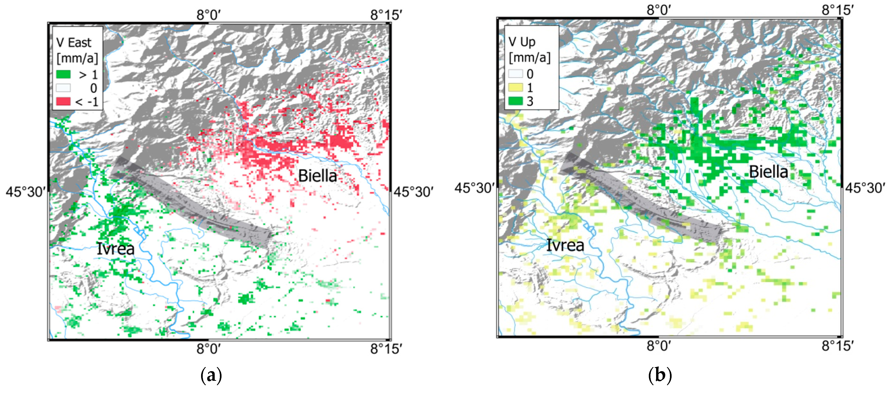
8.1.1. Biella—OrtaWestern Kinematic Zone

Placed along the Alps—Po plain border in the Eastern Piedmont Alps, this WKZ (Figure 9) lies on the periphery of the Pennidic dome, an area in which PS vertical velocities show a strong uplift as detected in past decades using “classical” geodetic methods [48] and that corresponds to the higher peaks of the entire Alpine mountain range. However, this WKZ shows stronger uplift than the surrounding areas. There is good agreement between the Western Iso-Kinematic Boundary (IKB) and a “normal” EKZ, the NNW-SSW valley of the Dora Baltea river and a scarp north of the Viverone lake in the morainic hills.

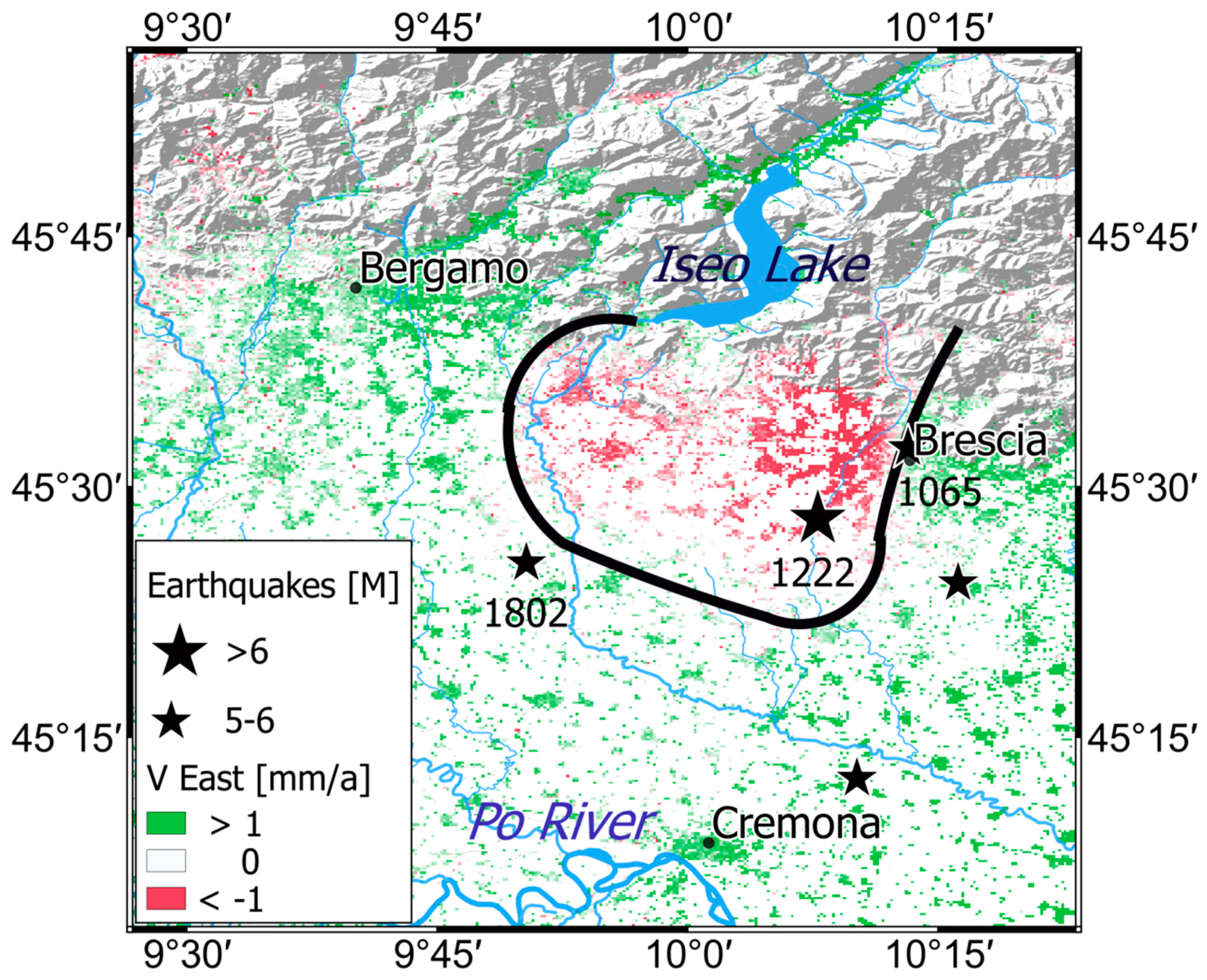
8.1.2. Brescia

The second selected area of subalpine WKZ is Brescia (Figure 10). East of the city, the IKB is characterized by strong inversions in the E/W PSI and N/S GPS velocities. In the plain, the IKB lies in a NS direction, prolonging from the Val Trompia. The western IKB, which is placed along the Orco river course, is also barely associated with a difference in the vertical components: subsidence characterizes the Brescia WKZ eastward, whereas the Bergamo “normal” EKZ (East-directed Kinematic zone) is currently uplifting. Intriguingly, the uplift stops near the IKB with the WKZ placed south of Como Lake. The westward movement of the Brescia area could be the origin of this uplift. This area hosts one of the highest seismic activities of the entirety of Lombardy; Brescia was hit by destructive earthquakes (Mw ≥ 5) on 27 March, 1065, and 25 December, 1222, the latter having a Mw ≥ 6. Another main shock of Mw 5.7 occurred near the town of Soncino on 12 May, 1802, which is located on the IKB. It is interesting to note that the 1222 and 1802 events were the only earthquakes with Mw ≥ 5.5 located west of Lake Garda in the central—northern part of the Po Plain [49].

A tectonic explanation of this situation must consider the complexity of the area, characterized by multiple and opposite thrusts imaged by seismic profiles, and that seismic activity is mostly related to blind faults that are buried under a thick cover of Plio—Pleistocene sediments, even if since 1965 some lightly isolated uplifts in the plain such as the Castenedolo and the Capriano del Colle uplift, the second also being the presumable epicenter of the 1222 earthquake, have been referenced to tectonic activity and not to geomorphological processes [50]. We can tentatively propose, however, that the anomaly might be confined in the Capriano del Colle Fault System, which is comprised of a south-vergent thrust in the plain and an associated high angle back thrust located at the border between the plain and the chain [51].

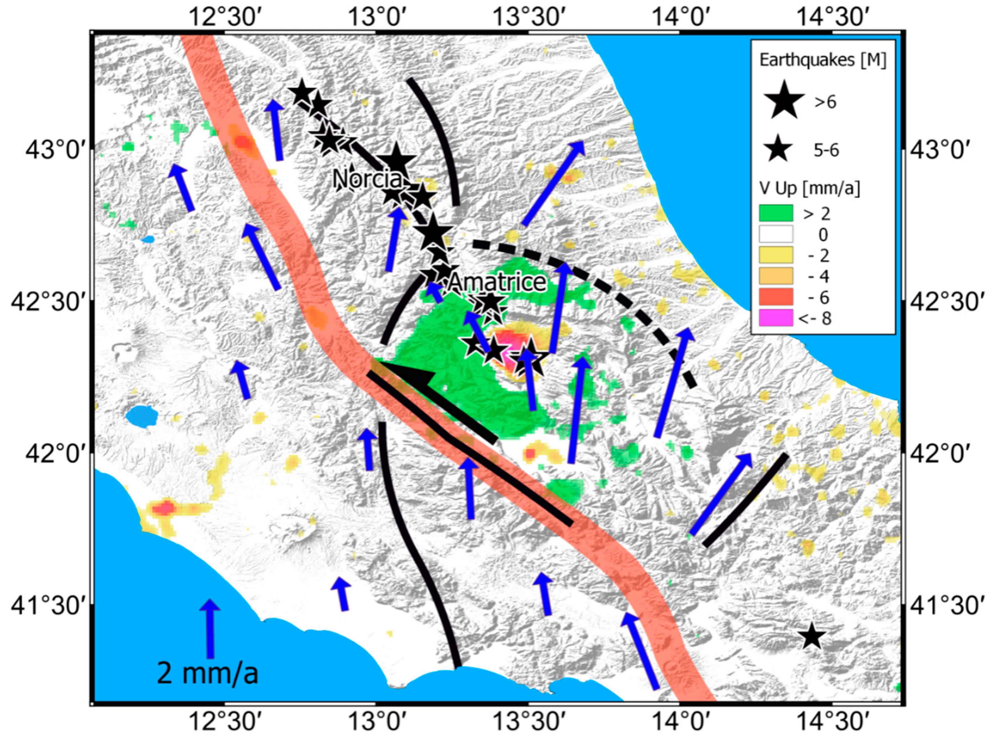
8.2. Central Italy

We have selected two areas in Central Italy, Abruzzi and Southern Latium, where PSI data fit the historical seismicity well, and propose an interesting view on local tectonics (Figure 11). Data suggest that the Central Apennines are a mosaic of many crustal wedges created by the Middle Pleistocene shortening along the Adriatic plate border [52].

8.2.1. Abruzzi

The Abruzzi Dome (AD) is an area of good agreement between topography, where the highest peaks of the Apenninic chain are grouped, and the vertical velocities, which show clear uplift. The AD barely corresponds also to a EKZ, with the exception of its north-western part, which belongs to a WKZ. The uplift of the AD can be explained by the horizontal velocity field; the SE limit is also an IKB between the EKZ of the AD and the channel of prevalent west-directed velocities of the Ortona–Roccamonfina system, marking the transition between Central and Southern Apennines [53]. In addition, the other borders of the AD are placed along main geological features: the Velino transtensive fault to the west, the Sibillini thrust front to the north, and the border between the Apennine belt and the deformed Adriatic foreland deposits to the East. More, the Velino fault is placed just over the Moho depth discontinuity that runs parallel to the Apenninic chain, marking in the Northern Apennines the limit between the extensional Tuscan domine and the compressional and uplifting Adriatic domine.

8.2.2. Southern Latium

PSI E-W data reveal a strong IKB, and there is also an IKB in the N-S GNSS components (even if they are not coincident, the much greater density of PSI data could explain the difference). This area is characterized by two Apennine–directed topographic lows, the Valle Latina and the Pontina plain, that are separated by the Lepini–Ausoni–Aurunci ridge. The PSI E-W IKB is clear and crosses these structures from the NW corner of the Valle Latina near Olevano Romano to the Tyrrhenian coast. Therefore, this IKB can be referred to as a possible southern continuation of the Olevano–Antrodoco thrust, with a reprise of the former structure in a new tectonic regime. The Italian Earthquake Parametric catalog [54] has poor records in this area, but it is interesting to observe that the epicenters of the few recorded events (16 January 1161 and 9 May 1170 Frusinate earthquakes and 15 October 1160 and 13 September 1348 Subiaco earthquakes) lie near this IKB. The 16 February 2013 M 4.8 Sora Earthquake epicenter (the major event between the 2009 and 2016 seismic sequences that affected the Central Apennines) instead lies near the eastern IKB of the isolated WKZ of SE Ernici mounts, like the 24 August 1877 Mw 5.2earthquake. These data suggest, as for the Brescia IKB, a relation between seismic activity and the variations in the velocity field.

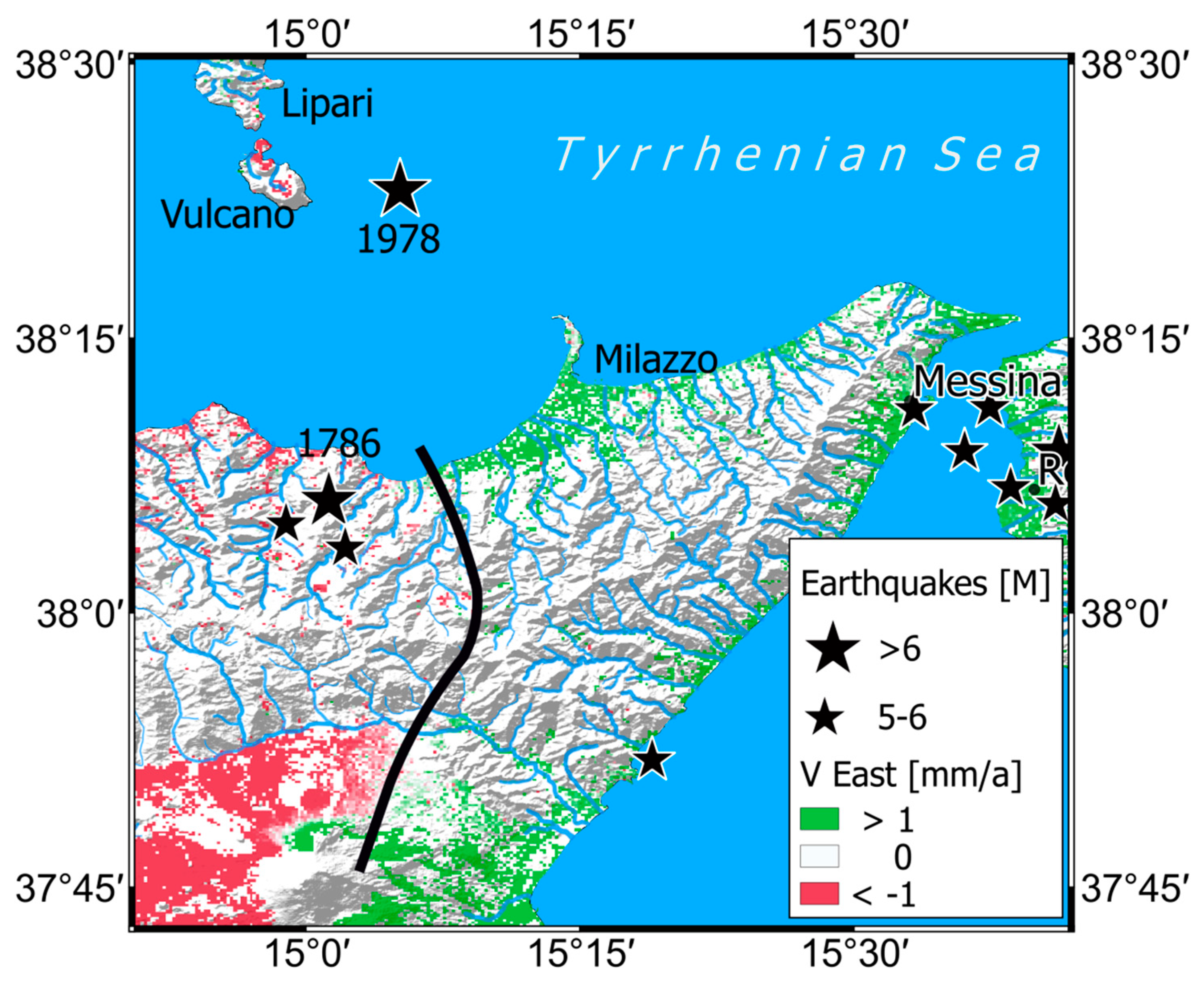
8.3. Southern Italy

In southern Italy, we have chosen NE Sicily (Figure 12), where the PSI data have a good chance of resolving the debate about the surface expression of the STEP fault (Slab Tear Edge Propagator) limiting the Ionian subduction slab to the SW, which also coincides with the limit between the extensional western side of the Calabro-Peloritan Arc (CPA) and the compressional belt of the Sicilian Fold-and-thrust-belt (SFTB). The CPA, which is sometimes considered to be an exotic terrane [55], is a nodal sector of the Apenninic—Maghrebid chain and is placed between the NW-SE-trending Southern Apennines and the EW—trending Siculo—Maghrebid chain. It differs from the adjoining sectors of the orogen because of the wide occurrence of the pre-Mesozoic crystalline basement that is not seen in either the southern Apennines or in the Siculo—Maghrebid chain and because it is the only segment of the whole orogen that still shows a wide submerged and deforming accretionary prism. The SFTB is made by the allochthonous nappes of the Neotethyan accretionary wedge that is thrusted onto the previously rifted passive margin of Africa. Offshore NW Sicily, Neotethyian units have been overthrusted by European margin units such as those of the CPA [56]. Post-Tortonian deformational events related to the opening of the Tyrrhenian Sea modified the pre-existing thrust geometry through the activation of a NW–SE-oriented dextral transcurrent fault system, affecting both offshore and onshore northern Sicily [57].

The hugely different earthquake mechanisms around this area demonstrate its tectonic complexity: extension in Calabria and NE Sicily, compression in northern Sicily and in the adjoining continental shelf, and strike-slip in the examined zone [28]. If there are no doubts that in the southern Thyrrenian continental platform the line beginning at Salina island arrives in the Patti Gulf area through Lipari and Vulcano, many authors have attempted to understand the position of this fault in NE Sicily and its prolongation in the Ionian Sea. This problem is still debated. The literature shows two solutions: the Tindari-Letojanni fault and the Taormina line. The Taormina line, proposed for example by Gallais et al. [58], is the thrust boundary along which the Calabrian units are superposed onto the Maghrebian (Sicilian) units.

The Tindari-Letojanni line crosses NE Sicily from the Tyrrhenian coast of the Gulf of Patti to the Jonian coast near Taormina Most of the authors prefer the Tindari—Letojanni as a segment of the Aeolian-Tindari-Letojanni Fault System (ATLFS) due its position along the Lipari—Vulcano volcanic alignment and the clustering of other major earthquakes in the Patti Gulf (Mw = 6.2, 10 March 1786 and Mw = 6.1 16 April 1978) and large numbers of minor events also on the mainland. This zone of deformation consists of a broad NNW trending system of faults that includes sets of right-lateral, left-lateral, and extensional faults as well as early strike-slip faults reworked under late extension [59]. Instead, the Taormina Line shows neither a similar market seismic activity nor current evidence of right-lateral decoupling [60].

The GPS velocities have clearly established that the CPA moves toward the NE, whereas the SFTB moves toward the NW. This is an ideal situation for a study of the EW component of the PSI data, which must well discriminate between a WKZ to the west (Madonie) and a EKZ to the east (Messina), the relative IKB being the surface expression of the STEP fault. The estimated motion of approximately 3.6 mm/a along the direction of 126° azimuth [61] results in a dextral transtension on the NNW-striking ATLF. The proposed surface expression of the ATLF is the Tindari–Novara fault zone [62], which is the western border of the Tindari–Barcellona triangular depression (TBTD), a lowland area filled with Plio–Quaternary sediments [63]. For many works the ATLF crosses the Ionian coast near Letojanni; for example, between the two GPS sites named ’TAOR’ and ’9532’, both stations being close to the city of Taormina [61].

This placement of the STEP makes the interpretation of the Etna and Hyblean volcanism problematic when they are considered as a product of the decompression of the mantle under the described transtensional conditions. This situation has been hypothesized before the STEP concept was theorized [64], but in this scenario, they are too far from the line, which causes the modeling of these magmas ascending in this very lateral position to be uncertain and difficult [65].

Instead, the PSI data suggest a different scenario either in the Tyrrhenian or on the Ionian coast. In the Patti gulf, the STEP crosses the coastline in a more easternmost position than previously thought, near Tonnarella di Furnari, just in front of the epicenter of the M 6.0 16 April 1978 earthquake, making the decoupling of the ATLF hypothesized near the coast [62] no longer necessary. In our scenario, the border fault of the TBTD is simply one of the various faults belonging to the transtensional deformed belt. Recent works show the lack of evidence of the ATFL south of Novara [63]; our data are poorer in this part, but the entirety of the Alcantara valley from Francavilla di Sicilia downstream clearly belongs to the Messina EKZ. Moreover, the occurrence in the Alcantara valley of the 28.6 ± 4.7 ka Monte Moio eruption cinder cone is worth noting; this volcanic structure is placed immediately proximate to our IKB, and since that eruption occurred in a very peripheral area of the Etna volcano and produced >10% pyroclasts, its batch of magma was a volatile-rich magma derived from depth and was not directly linked to the central conduit of the Ellittico volcano [66].

This volcanic episode occurred before the current Mongibello activity and during the former activity of the Ellittico volcano when magma-intrusion processes were unaffected by either the large Valle del Bove depression or the preferential weakness zones that facilitated the intrusion of magma along the slopes of the current volcano edifice. In this framework, flank eruptions as at Mt. Moio that were located outside the volcanic edifice were strictly controlled by the regional tectonic stress field. Moreover, the orientation of the Mt. Moio eruptive fissure is in agreement with the direction of the IKB, suggesting a correlation between this activity and the occurrence under it of the STEP fault bordering the Calabrian slab.

For these reasons, we can infer that the surface expression of the STEP fault line south of Novara di Sicilia will continue toward Castiglione di Sicilia, in the Monte Calcinera ridge, disappearing a few kilometers southward and buried under Mount Etna volcanic, as in Govers and Wortel (2005) [67]: we therefore propose a new name for the surface expression of the edge of the Calabrian slab: the Aeolian-Tonnarella-Castiglione di Sicilia Fault System (ATCFS). In this scenario, Etna Volcano also lies on the edge of the surface projection of the Calabrian slab, and moreover, the occurrence of the volcano can be referenced to the point at which the southward prolongation of the Ionian slab meets the other transtensionalthat is barely perpendicular to the Kumeta–Alcantara line, which is another main tectonic lineament of Sicily that runs parallel to its northern coast some 20 km inland. Therefore, the magmatic activity can be related to a pressure drop in the mantle at the intersection of these two transtensive lines. Because PSI data cannot be collected offshore, we are unable to discriminate between the three main proposed solutions for the currently debated continuation of the slab limit in the Ionian Sea; it continues near Mt. Etna as the Hyblean-Maltese escarpment fault (HMEF),which, for several authors [63], is an old lineament that has been rejuvenated many times the Etna-Alfeo fault [68] and the Ionian fault [69].Our work, which moves the point at which the line crosses the Ionian Sicilian coast from Letojanni (as in the literature) far to the south, placing it south of Catania, supports the picture of the southern continuation of the Calabrian slab limit along the HMEF.

9. Conclusions

GNSSs represent powerful instruments to realize global reference systems and to collect data for geodynamic interpretation. The DInSAR interferometric analysis represents a well-known and powerful technique used to detect and monitor surface motions of unstable areas at detailed scales such as those of unstable buildings [70,71,72] and landslides [4,6,13,15] as well as more widespread phenomena such as the subsidence and uplift zones [5,7,16,45].

Because it is impossible to know a priori the velocities of the ground reference points used for stacking the acquired SAR images, knowledge of the relative motion between the ground reference points of SAR images plays a fundamental role in obtaining correct DInSAR velocities: if the relative motion between ground reference points can be assumed constant within a restricted area, this hypothesis is not suitable for larger areas (i.e., on regional, continental or worldwide scales), and the GNSS geodetic velocity field must be applied to achieve a correct result.

In the present work, a method for creating a single and unique surface motion map by merging different datasets is presented. In this method, geodesy plays an important role in the datum alignment of the SAR products.

Combining these techniques (GNSS and SAR) improves researchers’ knowledge of surface movements for the following reasons:

• The surface movement maps present detailed and correct information that is coherent at a wider scale. It improves knowledge of geodynamic processes such as crustal dynamics, subsidence and uplift.
• The geodynamics can be improved by SAR data that verify the stability of GNSS sites. In fact, it can be used to check and highlight possible local movement involving a given GNSS site and then exclude it for geodetic purposes (i.e., crustal dynamics and reference frame).
• The SAR interferometry maps can be corrected for constant movements and for the low wave number components of the velocity field before being aligned to geodetic data.
• Because the different systems of acquisition used in SAR satellite missions produce velocity surfaces with different characteristics, it is necessary to create a unique surface motion map. Geodesy plays a fundamental role in the alignment of data before stacking SAR maps. The method of data analysis presented in this work should be applied taking account of other technologies such as LIDAR and leveling networks and particularly for validating DInSAR from newer SAR systems such as Sentinel-1, Cosmo-SkyMed SAR, and TerraSAR-X.
• The present work can be the base for the determination of a detail strain rate map of the Italian peninsula that plays an important role for a better understanding of geodynamical and geophysical processes [73].

References

- Bruyninx, C.; Becker, M.; Stangl, G. Regional densification of the IGS in Europe using the EUREF permanent GPS network (EPN). Phys. Chem. Earth Part A Solid Earth Geod. 2001, 26, 531–538. [Google Scholar] [CrossRef]
- Falchi, U.; Parente, C.; Prezioso, G. Global geoid adjustment on local area for GIS applications using GNSS permanent station coordinates. Geod. Cartogr. 2018, 44, 80–88. [Google Scholar] [CrossRef]
- Farolfi, G.; Del Ventisette, C. Monitoring the Earth’s ground surface movements using satellite observations: Geodinamics of the Italian peninsula determined by using GNSS networks. In Proceedings of the 2016 IEEE Metrology for Aerospace (MetroAeroSpace), Florence, Italy, 22–23 June 2016; pp. 479–483. [Google Scholar] [CrossRef]
- Del Soldato, M.; Riquelme, A.; Bianchini, S.; Tomàs, R.; Di Martire, D.; De Vita, P.; Calcaterra, D. Multisource data integration to investigate one century of evolution for the Agnone landslide (Molise, southern Italy). Landslides 2018, 15, 2113–2128. [Google Scholar] [CrossRef]
- Bianchini, S.; Raspini, F.; Solari, L.; Del Soldato, M.; Ciampalini, A.; Rosi, A.; Casagli, N. From Picture to Movie: Twenty Years of Ground Deformation recording over Tuscany Region (Italy) with Satellite InSAR. Front. Earth Sci. 2018, 6, 177. [Google Scholar] [CrossRef]
- Colesanti, C.; Ferretti, A.; Prati, C.; Rocca, F. Monitoring landslides and tectonic motions with the Permanent Scatterers Technique. Eng. Geol. 2003, 68, 3–14. [Google Scholar] [CrossRef]
- Raspini, F.; Bianchini, S.; Ciampalini, A.; Del Soldato, M.; Solari, L.; Novali, F.; Casagli, N. Continuous, semi-automatic monitoring of ground deformation using Sentinel-1 satellites. Sci. Rep. 2018, 8, 7253. [Google Scholar] [CrossRef] [PubMed]
- Santoro, M.; Askne, J.I.; Wegmuller, U.; Werner, C.L. Observations, modelling, and applications of ERS-ENVISAT coherence over land surfaces. IEEE Trans. Geosci. Remote Sens. 2007, 45, 2600–2611. [Google Scholar] [CrossRef]
- Crosetto, M.; Monserrat, O.; Cuevas-González, M.; Devanthéry, N.; Crippa, B. Persistent Scatterer Interferometry: A review. Int. J. Photogramm. Remote Sens. 2016, 115, 78–89. [Google Scholar] [CrossRef]
- Ferretti, A.; Prati, C.; Rocca, F. Permanent Scatterers in SAR Interferometry. IEEE Trans. Geosci. Remote Sens. 2001, 39, 8–20. [Google Scholar] [CrossRef]
- Goel, K.; Adam, N. A distributed scatterer interferometry approach for precision monitoring of known surface deformation phenomena. IEEE Trans. Geosci. Remote Sens. 2014, 52, 5454–5468. [Google Scholar] [CrossRef]
- Even, M.; Schulz, K. InSAR deformation analysis with distributed scatterers: A review complemented by new advances. Remote Sens. 2018, 10, 744. [Google Scholar] [CrossRef]
- Tofani, V.; Raspini, F.; Catani, F.; Casagli, N. Persistent Scatterer Interferometry (PSI) technique for landslide characterization and monitoring. Remote Sens. 2013, 5, 1045–1065. [Google Scholar] [CrossRef]
- Bekaert, D.P.S.; Segall, P.; Wright, T.J.; Hooper, A.J. A network inversion filter combining GNSS and InSAR for tectonic slip modeling. J. Geophys. Res. Solid Earth 2016, 121, 2069–2086. [Google Scholar] [CrossRef]
- Komac, M.; Holley, R.; Mahapatra, P.; van der Marel, H.; Bavec, M. Coupling of GPS/GNSS and radar interferometric data for a 3D surface displacement monitoring of landslides. Landslides 2015, 12, 241–257. [Google Scholar] [CrossRef]
- Del Soldato, M.; Farolfi, G.; Rosi, A.; Raspini, F.; Casagli, N. Subsidence Evolution of the Firenze–Prato–Pistoia Plain (Central Italy) Combining PSI and GNSS Data. Remote Sens. 2018, 10, 1146. [Google Scholar] [CrossRef]
- Bertotti, G.; Mosca, P.; Juez, J.; Polino, R.; Dunai, T. Oligocene to Present kilometres scale subsidence and exhumation of the Ligurian Alps and the Tertiary Piedmont Basin (NW Italy) revealed by apatite (U–Th)/He thermochronology: Correlation with regional tectonics. Terra Nova 2006, 18, 18–25. [Google Scholar] [CrossRef]
- Lustrino, M.; Morra, V.; Melluso, L.; Brotzu, P.; D’Amelio, F.; Fedele, L.; Franciosi, L.; Lonis, R.; Petteruti-Liebercknecht, A.M. The Cenozoic igneous activity of Sardinia. Period. Mineral. 2004, 73, 105–134. [Google Scholar]
- Spakman, W.; Wortel, M.J.R. A tomographic view on western Mediterranean geodynamics. In The TRANSMED Atlas, the Mediterranean Region from Crust to Mantle; Cavazza, W., Roure, F., Spakman, W., Stampfli, G.M., Ziegler, P., Eds.; Springer: Berlin/Heidelberg, Germany, 2004; pp. 31–52. [Google Scholar]
- Wortel, M.J.R.; Spakman, W. Structure and dynamics of subducted lithosphere in the Mediterranean region. Proc. van de Koninklijke NederlandseAcademie van Wetenschappen 1992, 95, 325–347. [Google Scholar]
- Rosenbaum, G.; Lister, G.S. Formation of arcuateorogenic belts in the western Mediterranean region. Geol. Soc. Am. Spec. Pap. 2004, 383, 41–56. [Google Scholar]
- Cocchi, L.; Passaro, S.; Caratori Tontini, F.; Ventura, G. Volcanism in slab tear faults is larger than in island-arcs and back-arcs. Nat. Commun. 2017, 8, 1451. [Google Scholar] [CrossRef]
- Serpelloni, E.; Bürgmann, R.; Anzidei, M.; Baldi, P.; Mastrolembo Ventura, B.; Boschi, E. Strain accumulation across the Messina Straits and kinematics of Sicily and Calabria from GPS data and dislocation modeling. Earth Planet. Sci. Lett. 2010, 298, 347–360. [Google Scholar] [CrossRef]
- Worth, J.R.; Spakman, W. Subduction and Slab Detachment in the Mediterranean-Carpathian Region. Science 2000, 290, 1910–1917. [Google Scholar]
- DISS Working Group. Database of Individual Seismogenic Sources (DISS), Version 3.2.1: A compilation of potential sources for earthquakes larger than M 5.5 in Italy and surrounding areas. 2018. Available online: http://diss.rm.ingv.it/diss/ (accessed on 10 February 2019). [CrossRef]
- Ustaszewski, K.; Schmid, S.M.; Fügenschuh, B.; Tischler, M.; Kissling, E.; Spakman, W. A map-view restoration of the Alpine-Carpathian-Dinaridic system for the Early Miocene. Swiss J. Geosci. 2008, 101 (Suppl. 1), S273–S294. [Google Scholar] [CrossRef]
- Fodor, L.; Jelen, B.; Marton, E.; Skaberne, D.; Car, J.; Vrabec, M. Miocene-Pliocene tectonic evolution of the Slovenian Periadriatic fault: Implications for Alpine-Carpathian extrusion models. Tectonics 1998, 17, 690–709. [Google Scholar] [CrossRef]
- Sani, F.; Vannucci, G.; Boccaletti, M.; Bonini, M.; Corti, G.; Serpelloni, E. Insights into the fragmentation of the Adria Plate. J. Geodyn. 2016, 102, 121–138. [Google Scholar] [CrossRef]
- Hooper, A. A multi-temporal InSAR method incorporating both persistent scatterer and small baseline approaches. Geophys. Res. Lett. 2018, 35. [Google Scholar] [CrossRef]
- Werner, C.L.; Hensley, S.; Goldstein, R.M.; Rosen, P.A.; Zebker, H.A. Techniques and applications of SAR interferometry for ERS-1: Topographic mapping, change detection, and slope measurement. In Proceedings of the First ERS-1 Symposium on Space at the Service of Our Environment, Cannes, France, 4–6 November 1996; Volume 1, pp. 205–210. [Google Scholar]
- Farolfi, G.; Del Ventisette, C. Contemporary crustal velocity field in Alpine Mediterranean area of Italy from new geodetic data. GPS Solut. 2015, 20, 715–722. [Google Scholar] [CrossRef]
- Farolfi, G.; Del Ventisette, C. Strain rates in the Alpine Mediterranean region: Insights from advanced techniques of data processing. GPS Solut. 2016, 21, 1027–1036. [Google Scholar] [CrossRef]
- Dach, R.; Hugentobler, U.; Fridez, P.; Meindl, M. The Bernese GPS Software Version 5.0; Astronomical Institute of University of Bern (AIUB): Bern, Switzerland, 2007. [Google Scholar]
- Böhm, J.; Heinkelmann, R.; Schuh, H.A. Global Model of Pressure and Temperature for Geodetic Applications. J. Geod. 2007, 81, 679–683. [Google Scholar] [CrossRef]
- Williams, S.D.P. CATS: GPS coordinate time series analysis software. GPS Solut. 2008, 12, 147–153. [Google Scholar] [CrossRef]
- Palano, M. On the present-day crustal stress, strain-rate fields and mantle anisotropypattern of Italy. Geophys. J. Int. 2015, 200, 969–985. [Google Scholar] [CrossRef]
- Herring, T.A.; King, R.W.; McClusky, S.C. Introduction to GAMIT/GLOB. Release 10.4; Massachusetts Institute of Technology: Cambridge, MA, USA, 2010; pp. 1–48. [Google Scholar]
- Herring, T. MATLAB Tools for viewing GPS velocities and time series. GPS Solut. 2003, 7, 194. [Google Scholar] [CrossRef]
- Zafiri, Z.; Nilfouroushan, F.; Raeesi, M. Crustal stress Map of Iran: Insight from seismic and geodetic computations. Pure Appl. Geophys. 2014, 171, 1219–1236. [Google Scholar] [CrossRef]
- Italian Geoportale Nazionale. Available online: www.pcn.minambiente.it (accessed on 20 December 2017).
- Shepard, D. A two-dimensional interpolation function for irregularly-spaced data. In Proceedings of the 1968 ACM National Conference, Las Vegas, NV, USA, 27–29 August 1968. [Google Scholar] [CrossRef]
- Bartier, P.; Keller, P. Multivariate interpolation to incorporate thematic surface data using inverse distance weighting (IDW). Comput. Geosci. 1996, 22, 795–799. [Google Scholar] [CrossRef]
- Lee, S.; Wolberg, G.; Shin, S.Y. Scattered Data Interpolation with Multilevel B-Splines. IEEE Trans. Vis. Comput. Graph. 1997, 3, 228–244. [Google Scholar] [CrossRef]
- Morelli, M.; Piana, F.; Mallen, L.; Nicolò, G.; Fioraso, G. Iso-Kinematic Maps from statistical analysis of PS-InSAR data of Piemonte, NW Italy. Comparison with geological kinematic trends. Remote Sens. Environ. 2011, 115, 1188–1201. [Google Scholar] [CrossRef]
- Farolfi, G.; Bianchini, S.; Casagli, N. Integration of GNSS and satellite InSARdta: Derivation of fine-scale vertical surface motion maps of Po Plain, Northern Apennines and Southern Alps, Italy. IEEE Trans. Geosci. Remote Sens. (TGRS) 2018. [Google Scholar] [CrossRef]
- Guidoboni, E.; Comastri, A. The “exceptional” earthquake of 3 January 1117 in the Verona area (northern Italy): A critical time review and detection of two lost earthquakes (lower Germany and Tuscany). J. Geophys. Res. 2005, 110, B12309. [Google Scholar] [CrossRef]
- Galli, P.; Galadini, F.; Pantosti, D. Twenty years of paleoseismology in Italy. Earth-Sci. Rev. 2008, 88, 89–117. [Google Scholar] [CrossRef]
- Nocquet, J.-M.; Calais, E. Geodetic Measurements of Crustal Deformation in the Western Mediterranean and Europe. Pure Appl. Geophys. 2004, 161, 661–681. [Google Scholar] [CrossRef]
- Albini, P.; Rovida, A. The 12 May 1802 earthquake (N Italy) in its historical and seismological context. J. Seismol. 2010, 14, 629–651. [Google Scholar] [CrossRef]
- Desio, A. I rilievi isolati della Pianura Lombarda e di movimenti tettonici del Quaternario. Rend. Ist. Lomb. Acc. Sci. Lett. Sez. A 1965, 99, 881–894. [Google Scholar]
- Livio, F.A.; Berlusconi, A.; Michetti, A.M.; Sileo, G.; Zerboni, A.; Trombino, L.; Cremaschi, M.; Mueller, K.; Vittori, E.; Carcano, C.; et al. Active fault-related folding in the epicentral area of the December 25, 1222 (Io=IXMCS) Brescia earthquake (Northern Italy): Seismotectonic implications. Tectonophysics 2009, 476, 320–335. [Google Scholar] [CrossRef]
- Mantovani, E.; Viti, M.; Cenni, N.; Babbucci, D.; Tamburelli, C.; Baglione, M.; D’Intinosante, V. Seismotectonics and present seismic hazard in the Tuscany–Romagna–Marche–Umbria Apennines (Italy). J. Geodyn. 2015, 89, 1–14. [Google Scholar] [CrossRef]
- Di Bucci, D.; Corrado, S.; Naso, G. Active faults at the boundary between Central and Southern Apennines (Isernia, Italy). Tectonophysics 2002, 359, 47–63. [Google Scholar] [CrossRef]
- Rovida, A.; Locati, M.; Camassi, R.; Lolli, B.; Gasperini, P. (Eds.) CPTI15, the 2015 version of the Parametric Catalogue of Italian Earthquakes; Istituto Nazionale di Geofisica e Vulcanologia: Rome, Italy, 2016. [Google Scholar] [CrossRef]
- Bonardi, G.; Cavazza, W.; Perrone, V.; Rossi, S. Calabria-Peloritaniterrane and northern Ionian Sea. In Anatomy of an Orogen: The Apennines and Adjacent Mediterranean Basins; Vai, G.B., Martini, I.P., Eds.; Springer: Dordrecht, The Netherland, 2001. [Google Scholar] [CrossRef]
- Roure, F.; Howell, D.G.; Muller, C.; Moretti, I. Late Cenozoicsubduction complex of Sicily. J. Struct. Geol. 1990, 12, 259–266. [Google Scholar] [CrossRef]
- Lentini, F.; Carbone, S.; Guarnieri, P. Collisional and post collisional tectonics of the Apenninic-Maghrebianorogen (southern Italy). GSA Spec. Pap. 2006, 409, 57–81. [Google Scholar] [CrossRef]
- Gallais, F.; Graindorge, D.; Gutscher, M.A.; Klaeschen, D. Propagation of a lithospheric tear fault (STEP) through the western boundary of the Calabrian accretionary wedge offshore eastern Sicily (Southern Italy). Tectonophysics 2013, 602, 141–152. [Google Scholar] [CrossRef]
- Billi, A.; Barberi, G.; Faccenna, C.; Neri, G.; Pepe, F.; Sulli, A. Tectonics and seismicity of the Tindari Fault System, southern Italy: Crustal deformations at the transition between on going contractional and extensional domains located above the edge of a subducting slab. Tectonics 2006, 25, TC2006. [Google Scholar] [CrossRef]
- Ghisetti, F.; Pezzino, A.; Atzori, P.; Vezzani, L. Un approccio strutturale per la definizione della Linea di Taormina: Risultati preliminari. Mem. Soc. Geol. Ital. 1991, 47, 272–283. [Google Scholar]
- Palano, M.; Ferranti, L.; Monaco, C.; Mattia, M.; Aloisi, M.; Bruno, V.; Cannavò, F.; Siligato, G. GPS velocity and strain fields in Sicily and southern Calabria, Italy: Updated geodetic constraints on tectonic block interaction in the central Mediterranean. J. Geophys. Res. 2012, 117, B07401. [Google Scholar] [CrossRef]
- Cultrera, F.; Barreca, G.; Ferranti, L.; Monaco, C.; Pepe, F.; Passaro, S.; Graziella, B.; Bruno, V.; Burrato, P.; Mattia, M.; et al. Structural architecture and active deformation pattern in the northern sector of the Aeolian-Tindari-Letojanni fault system (SE Tyrrhenian Sea-NE Sicily) from integrated analysis of eld, marine geophysical, seismological and geodetic data. Ital. J. Geosci. 2017, 136, 399–417. [Google Scholar] [CrossRef]
- Di Stefano, A.; Lentini, R. Ricostruzione stratigrafica e significato paleotettonico dei depositi plio-pleistocenici del margine tirrenico tra Villafranca Tirrena e Faro (Sicilia nordorientale). Stud. Geol. Camerti 1995, 2, 219–237. [Google Scholar]
- Doglioni, C.; Innocenti, F.; Mariotti, G. Why Mt Etna? Terra Nova 2001, 13, 25–31. [Google Scholar] [CrossRef]
- Neri, M.; Rivalta, E.; Maccaferri, F.; Acocella, V.; Cirrincione, R. Etnean and Hyblean volcanism shifted away from the Malta Escarpment by crustal stresses. Earth Planet. Sci. Lett. 2018, 486, 15–22. [Google Scholar] [CrossRef]
- Del Carlo, P.; Branca, S.; De Beni, E.; Lo Castro, M.D.; Wijbrans, J.R. The Mt. Moio eruption (Etna): Stratigraphy, petrochemistry and 40Ar/39Ar age determination with inferences on the relationship between structural setting and magma intrusion. J. Volcanol. Geotherm. Res. 2012, 241–242, 49–60. [Google Scholar] [CrossRef]
- Govers, R.; Wortel, M.J.R. Lithosphere tearing at STEP faults: Response to edges of subduction zones. Earth Planet. Sci. Lett. 2005, 236, 505–523. [Google Scholar] [CrossRef]
- Argnani, A. The Southern Tyrrhenian subduction system: Recent evolution and neotectonic implications. Ann. Geophys. 2000, 43, 585–607. [Google Scholar]
- Polonia, A.; Torelli, L.; Gasperini, L.; Cocchi, L.; Muccini, L.; Bonatti, E.; Hensen, C.; Schmidt, M.; Romano, A.; Artoni, A.; et al. Lower plate serpentinite diapirism in the Calabrian Arc subduction complex. Nat. Commun. 2017, 8, 2172. [Google Scholar] [CrossRef]
- Di Pasquale, A.; Nico, G.; Pitullo, A.; Prezioso, G. Monitoring Strategies of Earth Dams by Ground-Based Radar Interferometry: How to Extract Useful Information for Seismic Risk Assessment. Sensors 2018, 18, 244. [Google Scholar] [CrossRef]
- Narayan, A.B.; Tiwari, A.; Devara, M.; Dwivedi, R.; Dikshit, O. Monitoring landslides in the Mussoorie region, Uttarakhand using multi-temporal SAR interferometry with Sentinel-1 images. Int. Arch. Photogramm. Remote Sens. Spat. Inf. Sci. 2008, XLII-5, 849–853. [Google Scholar] [CrossRef]
- Tiwari, A.; Narayan, A.B.; Devara, M.; Dwivedi, R.; Dikshit, O. Multi-sensor geodetic approach for landslide detection and monitoring. ISPRS Ann. Photogramm. Remote Sens. Spat. Inf. Sci. 2018, IV-5, 287–292. [Google Scholar] [CrossRef]
- Neres, M.; Custódio, C.; Custódio, S.; Palano, M.; Fernandes, R.; Matias, L.; Carafa, M.; Terrinha, P. Gravitational Potential Energy in Iberia: A Driver of Active Deformation in High-Topography Regions. J. Geophys. Res. Solid Earth 2017, 123, 10277–10296. [Google Scholar] [CrossRef]
- QGIS Development Team. QGIS Geographic Information System. Open Source Geospatial Foundation, 2009. Available online: http://qgis.org (accessed on 10 February 2019).
- Ramsey, P. Postgis Manual; Refractions Research Inc.: Victoria, BC, Canada, 2005. [Google Scholar]
- Conrad, O.; Bechtel, B.; Bock, M.; Dietrich, H.; Fischer, E.; Gerlitz, L.; Wehberg, J.; Wichmann, V.; Böhner, J. System for Automated Geoscientific Analyses (SAGA) v. 2.1.4. Geosci. Model. Dev. 2015, 8, 1991–2007. [Google Scholar] [CrossRef]
- Farr, T.G.; Rosen, P.A.; Caro, E.; Crippen, R.; Duren, R.; Hensley, S.; Kobrick, M.; Paller, M.; Rodriguez, E.; Roth, L.; et al. The Shuttle Radar Topography Mission. Rev. Geophys. 2007, 45, RG2004. [Google Scholar] [CrossRef]
© 2019 by the authors. Licensee MDPI, Basel, Switzerland. This article is an open access article distributed under the terms and conditions of the Creative Commons Attribution (CC BY) license (http://creativecommons.org/licenses/by/4.0/).
Share and Cite
Farolfi, G.; Piombino, A.; Catani, F. Fusion of GNSS and Satellite Radar Interferometry: Determination of 3D Fine-Scale Map of Present-Day Surface Displacements in Italy as Expressions of Geodynamic Processes. Remote Sens. 2019, 11, 394. https://doi.org/10.3390/rs11040394
Farolfi G, Piombino A, Catani F. Fusion of GNSS and Satellite Radar Interferometry: Determination of 3D Fine-Scale Map of Present-Day Surface Displacements in Italy as Expressions of Geodynamic Processes. Remote Sensing. 2019; 11(4):394. https://doi.org/10.3390/rs11040394
Chicago/Turabian StyleFarolfi, Gregorio, Aldo Piombino, and Filippo Catani. 2019. "Fusion of GNSS and Satellite Radar Interferometry: Determination of 3D Fine-Scale Map of Present-Day Surface Displacements in Italy as Expressions of Geodynamic Processes" Remote Sensing 11, no. 4: 394. https://doi.org/10.3390/rs11040394