Separation and Recovery of Geophysical Signals Based on the Kalman Filter with GRACE Gravity Data
by
 , and
, and
Xiaolong Wang
1 ,
,
Zhicai Luo
2,3,*,
Bo Zhong
1,4, 
Yihao Wu
5,6,
Zhengkai Huang
7,
Hao Zhou
2 and
Qiong Li
2 1
School of Geodesy and Geomatics, Wuhan University, Wuhan 430079, China
2
MOE Key Laboratory of Fundamental Physical Quantities Measurement, Hubei Key Laboratory of Gravitation and Quantum Physics, Institute of Geophysics, School of Physics, Huazhong University of Science and Technology, Wuhan 430074, China
3
Collaborative Innovation Center of Geospatial Technology, Wuhan University, Wuhan 430079, China
4
Key Laboratory of Geospace Environment and Geodesy, Ministry of Education, Wuhan University, Wuhan 430079, China
5
School of Earth Sciences and Engineering, Hohai University, Nanjing 210098, China
6
State Key Laboratory of Geodesy and Earth’s Dynamics, Institute of Geodesy and Geophysics, Chinese Academy of Sciences, Wuhan 430077, China
7
School of Civil Engineering and Architecture, East China Jiaotong University, Nanchang 330013, China
*
Author to whom correspondence should be addressed.
Remote Sens. 2019, 11(4), 393; https://doi.org/10.3390/rs11040393
Submission received: 31 December 2018
/
Revised: 8 February 2019
/
Accepted: 11 February 2019
/
Published: 15 February 2019
(This article belongs to the Special Issue GRACE Facing the Challenge of Extreme Spatial and Temporal Scales)
Abstract
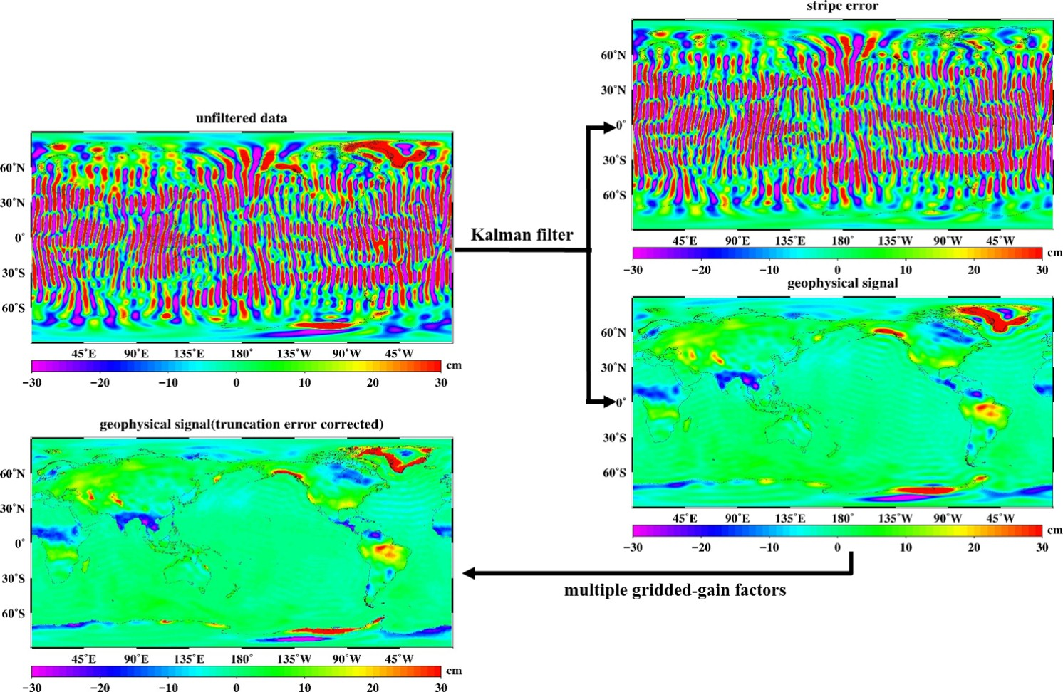
:Monthly gravitational field solutions as spherical harmonic coefficients produced by the GRACE satellite mission require post-processing to reduce the effects of shortwave-length noises and north–south stripe errors. However, the spatial smoothing and de-striping filter commonly used in the post-processing step will either reduce spatial resolution or remove short-wavelength features of geophysical signals, mainly at high latitudes. Here, by using prior covariance information that reflects the spatial and temporal features of the geophysical signals and the correlated errors derived from the synthetic model, together with the covariance matrix of the formal errors for the monthly gravity spherical harmonic coefficients, we apply the Kalman filter to separate the geophysical signal from GRACE Level-2 data and simultaneously to estimate the correlated errors. By increasing the number of observations, the iterative process is applied to update the state vector and covariance in the Kalman filter because the prior information is not accurate. Due to the inevitable truncation error, multiple gridded-gain factors method considering different temporal frequencies has been developed to recover the geophysical signal. The results show that the Kalman filter can reduce the high-frequency noises and correlated errors remarkably. When compared with the commonly used filter, no spatial filter (such as Gaussian filter) is used in the Kalman filter. Therefore, the estimated signal preserves its natural resolution, and more detailed information is retained. It shows good consistency when compared with mascon solutions in both secular trend and annual amplitude.

1. Introduction
After more than 15 productive years in orbit, the U.S./German Gravity Recovery and Climate Experiment (GRACE) satellite mission has provided unprecedented insights into how our planet is changing (mainly the surface mass variations) by tracking the continuous movement of liquid water, ice, and the solid Earth [1]. Generally, there are two categories of processing methods to obtain the surface mass variations from the GRACE observations. The first one is the mascon approach, directly using the intersatellite range-rate and acceleration observation to estimate the mass changes of mass concentration blocks (or “mascons”) on the Earth’s surface [2,3,4]. These mascon solutions are computed in presence of regularization constraint and no additional smoothing or empirical de-striping or filtering is applied. The second approach uses the monthly gravity field solutions (GRACE Level-2 data) as spherical harmonic (SH) Stokes coefficients provided by GRACE analysis centers [5]. Due to the errors of the satellite instruments and the imperfections of the background models [6], the SH coefficients are seriously polluted by errors. Therefore, the direct use of GRACE Level-2 data to measure the surface mass changes of the Earth is affected by different kinds of noises, and if they are not filtered in the post processing, it is difficult to extract useful geophysical signals from the Level-2 data.
The noises among the Level-2 data are mainly manifested in two types. One is the high-frequency (short-wavelength) noise, namely mainly existing in the high degree part of the gravity field. And the other is the north–south stripe error which is shown as north–south stripe distribution features. In order to obtain the pure geophysical signals, it is necessary to isolate the signals from the SH coefficients accurately. The principle of the separation is to obtain the signals as completely as possible (without any attenuation or damage) from the global observations of the GRACE mission. To solve this problem, many algorithms have been proposed.
One type of the algorithms is spatial smoothing filtering method mainly to weaken the impact of high-frequency noise. The first such filter is the degree-dependent isotropic Gaussian filter [5,7]. The higher degree of the SH coefficients, the more serious the effect caused by high-frequency noise is. Therefore, by reduction of the weight of high degree of the SH coefficients, this filter can obviously reduce the effects of the shortwave-length noise. Unlike the isotropic Gaussian filter, the non-isotropic filter [8], such as Fan filter [9], is constructed depending on both the degree and the order of the SH coefficients, and it has been proved to be a better method. The nature of this type of methods is to achieve a smooth effect by sacrificing spatial resolution of signals. Therefore, the selection of the smoothing radius of the filter is a problem. Only if the smoothing radius is large enough can the noise be eliminated significantly and can the signal be clearly displayed. However, the short-wavelength features of the original signals will be removed, and simultaneously the original spatial resolution will also be destroyed. Moreover, the smoothing radius will change with time and latitude, since the satellite orbit height changes with time, and the data on different latitudes on the Earth will have different spatial resolution. For example, a smoothing radius of 350 km may be appropriate for areas near the equator, but it is too large for denser ground track coverage near the poles. Another problem of this spatial smoothing filtering method is that it will yield signal leakage. Even though researchers have put forward the forward-modeling method [10] and the scaling technique [11,12,13,14,15] to restore the signal, and the effect is obvious, the signals cannot be completely restored.
Focusing on the north–south stripe errors, Swenson and Wahr [16] developed another type of algorithm called the de-striping filter, which aims to reduce the empirical errors owing to certain even–odd degree correlations found in the GRACE SH coefficients. Duan et al. [17] empirically designed a moving window filter to reduce these correlations. The core idea of this kind of filtering method is to use the polynomial to fit the correlation errors between certain SH coefficients. Next, by subtracting the fitted values from the original SH coefficients, the residual values are treated as the signals. The de-striping filter for the Stokes’ coefficients with order m or higher using a polynomial of degree n is also known as the PnMm filter, such as P7M7 and P11M11 [18], P3M10 [19], P3M6 [20,21], P4M6 [22],and P5M8 [23]. Different values of the parameter n and m in the de-striping filter can suppress the stripe features to a different extent in different research contexts. However, there are still many stripe features around the equator area after they are by de-striping filter method. After that, a spatial smoothing filtering method such as Gaussian or Fan smoothing is usually required. The so-called correlation and the parameters n and m are all empirical, so they cannot be accurately obtained. Because of a certain width of the moving window, the high order parts of the SH coefficients which have much more serious north–south stripe errors cannot be filtered [9]. Moreover, some shortwave-length features of the geophysical signals are removed after this filter method, mainly at high latitudes [16].
In addition to the algorithms above, some other algorithms have also been proposed to filter the observations to obtain useful signals. Chen et al. [24] constructed an optimized smoother based on a criterion of maximizing the ratio of variance over land relative to that over the oceans to suppress high-degree noise in the monthly gravity field solutions. Empirical orthogonal function (EOF) analysis [25,26] was developed to extract signals from the GRACE Level-2 data. Frappart et al. [27] denoised satellite gravity signals by independent component analysis (ICA).
Even though the filtering methods described above can successfully suppress the high-frequency noise and the north–south stripe errors, they do not take advantage of the prior information. Therefore, it is impossible to obtain the rigorous estimates of north–south stripe errors of SH coefficients and the signals are also suppressed at the same time. However, using some prior information that reflects both the spatial spectral features and temporal correlations among the data, Kurtenbach et al. [28] obtained daily gravity field solutions based on GRACE Level 1B data. Wang et al. [29] developed a new stochastic filter technique for the statistically rigorous separation of gravity signals and correlated “stripe” noises in the GRACE Level-2 data. This stochastic filter is able to remove the correlated stripe noise even without a spatial smoothing procedure. However, the stochastic model designed to reflect monthly GRACE correlated errors for all months is not time-varying, so this is not in line with the actual situation.
The study in this article is inspired by Kurtenbach et al. [28] and Wang et al. [29], who focused on the construction of stochastic models and used the Kalman filter to improve GRACE gravity field solutions. The correction of the truncation error is also the subject of our research. The main contents of this article are as follows: In Section 2, the Kalman filter approach is explained, and the prior covariance information used in the Kalman filter and multiple gridded-gain factors to correct the truncation error are given. Section 3 shows the results, and Section 4 is the discussion. Conclusions are presented in Section 5.
2. Methods
2.1. The Kalman Filter Approach
The surface mass temporal variations of the Earth can be expressed by the GRACE-derived SH coefficients. Due to the errors mentioned above, we can consider the SH coefficients are composed of geophysical signal, north–south stripe error, and a zero-mean Gaussian white noise. Therefore, the observation equations for the GRACE observations (Level-2 data) in time (i.e., a particular month) can be formulated as follows [29]:
where is the GRACE SH coefficients as the observation vector in time , is the design matrix, is the unknown state vector which contains geophysical signal and stripe noise , and is the Gaussian white noise with covariance matrix of the GRACE SH coefficients. Commonly, the degree of the monthly GRACE solutions is truncated to 60, so there are a total of 7434 unknown parameters in the state vector , and the design matrix is a sparse matrix of dimension 3717 × 7434.
Obviously, this is an ill-posed problem because the number of unknown parameters is twice the number of observations. Up to now, no temporal correlations have been introduced into the processing strategy. However, it can be safely predicted that the estimate of the gravity field will not change arbitrarily from one month to the next. Therefore, we can assume a simplified case that the time evolution of the gravity field is a linear process and can be written as the following first order Markov process [28]:
This represents a prediction of the gravity field coefficients from month to the current month . The prediction is characterized by the matrix of the process dynamic , namely the state transition matrix. is process noise and we assume that it is zero mean with covariance matrix (including covariance matrix of geophysical signal and stripe noise):
This is different from Wang et al. [29]; they assumed the stripe noise is uncorrelated with the temporal changes of the geophysical signal. Therefore, the part of the state transition matrix representing the stripe noise is a zero matrix, and the covariance matrix is the same for every month. However, since the evolving state of the GRACE flight segment will lead to varying errors in each monthly field over time [30], this is not consistent with the actual situation. Therefore, the state transition matrix here is a diagonal matrix, and time-varying month-by-month stochastic models of monthly GRACE correlated errors based on GRACE data quality information need be designed.
Based on the above assumptions and analysis, we can use standard Kalman filter formulation to estimate the state vector at the current month. The standard Kalman filter approach is divided into two steps: prediction and update. In the prediction step, the state of the current epoch is predicted by the previously updated state. Therefore, the previously updated state vector, with its covariance matrix, and the time-varying covariance matrix of process noise should be known. When in the update step, new observations (namely the monthly GRACE solutions) of the current epoch are included, and the predictions of the current epoch are improved by these observations. The Gaussian white noise with covariance matrices of these observations are also needed. Therefore, the construction of the previously updated state vector and the covariance matrices and are crucial in the Kalman filter. The design matrix and the state transition matrix are also important, and they are determined in this section.
It is clear that the prior information will have a significant impact on the filtering results. However, the synthetic model as the prior information is not accurate for various reasons. It is inevitable that the prior models have a variety of errors, but we can improve the accuracy and reliability of the results by increasing the number of observations. Here, we introduce an iterative process. The four sets of monthly gravity solutions and covariance matrices obtained by CSR [30], GFZ [31], JPL [32], and ITSG-Grace2014 [33] are introduced into the iterative process as observations. Firstly, the GRACE Level-2 data provided by the first analysis center is combined with the constructed prior information, so a solution through Kalman filtering can be obtained. The solution obtained in the first step is then taken as the prior information and combined with the GRACE Level-2 data provided by the second analysis center, so another solution is obtained by Kalman filtering. In the same way, the solutions from the remaining two analysis centers are incorporated into the iteration process. The observations, the state vectors, and the covariance matrices are updated in each iteration. Therefore, the final filtered result fuses the information of the solutions of each GRACE analysis center.
2.2. Prior Information
As we know, the estimated state at the current month depends on prior information, such as the earlier states and the associated covariance matrices in the Kalman filter approach. Therefore, a previously updated state vector with its covariance matrix as well as the time-varying process noise covariance matrix and the covariance matrix of the observational white noise as mentioned above should be determined. The acquisition and construction of the prior information and the associated covariance matrices used in the Kalman filter procedure are described in this section.
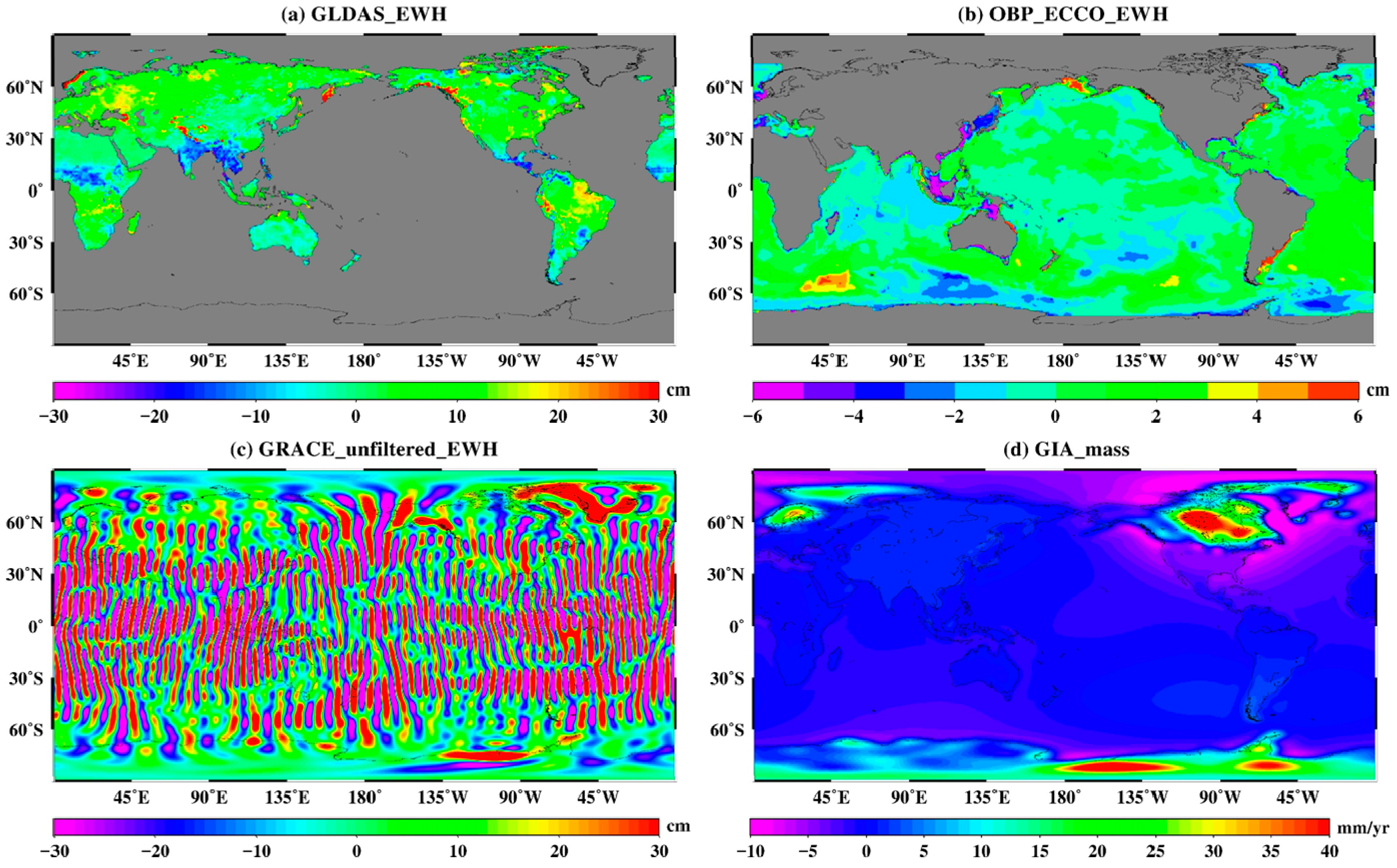
The geophysical signals detected by the GRACE satellites are the sum of terrestrial water storage changes, ocean mass variations, glacial isostatic adjustment (GIA), and the evolution of other geophysical phenomena [1]. In order to obtain prior information on the surface mass variation of the entire planet, we should make full use of various models and observations related. Here, we combine the global mass variations from the Global Land Data Assimilation System (GLDAS) land water content model [11], the GRACE-derived monthly mass variations (as in some regions, such as Antarctica and Greenland, few models are available), and the ocean bottom pressure (OBP) model [34], together with a GIA model [35], as synthetic monthly models (see Figure 1) that offer the prior information of the geophysical signals.
The monthly mass variations of all the synthetic models are truncated to degree 60, and we take the truncated SH coefficients of the synthetic models as the previously updated state of the geophysical signals. Therefore, drawing on the idea of degree variance [29,36], we can design the diagonal components of the SH coefficients variances as the matrix (Figure 2(a)). It is divided into two parts (coefficients of cosine and sine) and expressed as follows:
where and are the differences between the truncated SH coefficients of two adjacent months’ synthetic models. The values of degree variance at all different orders of the SH coefficients are the same when given a certain degree . It should be noted that the assumption that the SH coefficients are not correlated with each other is made here, so the matrix is diagonal.
However, no model or observation can be used to estimate the prior information of the stripe noise currently. According to the characteristics of the stripe error, Wang et al. [29] designed the matrix with a number of trials and choices. Therefore, the design is empirical and statistical. Most importantly, the covariance matrix does not change with the month, and this does not match the reality. By comparing the unfiltered results with the filtered results (traditionally, the PnMm filter and spatial smoothing such as Gaussian smoothing are adopted) expressed as the equivalent water height (EWH), we can find that the stripe noise is dominant in the observation, and almost no obvious signal can be used, especially in the middle and low latitudes. This is why the original GRACE Level-2 data needs to be post-processed. Thus, the original observation subtracted from the filtered result can be considered as the approximation of the time-varying stripe error. Although this is an approximation, since the magnitude of the stripe error is much larger than the magnitude of the geophysical signal, this approximation is very close to the true value of the stripe error. It should be noted that the spatial filtering here can only be Gaussian smoothing, because the PnMm filtering can significantly change the signal, especially in high latitudes [16]. Therefore, we can take the approximation as the previously updated state of the stripe noise. Similarly, we can also calculate the diagonal components the covariance matrix (Figure 2b) according to Equation (4).
Owing to the errors in the model and observation, and to the approximation of the error, these are just approximate estimates of the signal and stripe error (although they prevail in the true signal and stripe error), but we can reduce the errors caused by these approximations by increasing the observations with an iterative process as mentioned in Section 2.1. Moreover, Wang et al. [29] had proved that increasing or decreasing the covariance in a certain range in the Kalman filter procedure does not have great effect on the results. Thus, in some way, using a highly accurate covariance is not urgently needed.
When the monthly gravitational field solutions are released by each GRACE analysis center, the formal errors that can describe the white noise of the observations for the SH coefficients are also released. Therefore, the formal errors can be directly used as the covariance of the observational white noise in the Kalman filter. We used four analysis center products. Among them, CSR and ITSG-Grace2014 provided the full formal error covariance matrices, but the formal error covariance matrices obtained by GFZ and JPL were only diagonal components. To examine the feasibility of the simplified diagonal covariance matrix, the results of using a diagonal matrix and a full matrix were compared. The result of the comparison is that the RMS (root mean square) difference in mass estimate expressed as the EWH is less than 1 cm. In addition, the quotient of the latitude-weighted RMS of the EWH of the continental and oceanic signals that represent the signal-to-noise ratio (SNR) [24] was calculated, and the results showed that the difference was not obvious. Therefore, we used the diagonal components of the formal errors as the observational covariance matrices when the full formal error covariance matrices were not accessible. Figure 2c shows the covariance matrix of the observation provided by CSR. It can be seen in Figure 2c that the values of the main diagonal elements are much larger than the elements of other locations, and this can partly explain the feasibility of using diagonal elements. Moreover, using the full covariance matrices greatly increases computation time and consumes a substantial amount of memory.
2.3. Multiple Gridded-Gain Factors
Based on the method described above, the geophysical signals expressed by SH coefficients can be separated from the GRACE monthly solutions by using the Kalman filter. Typically, the geophysical signal is truncated to a certain spectral degree (60 in this article). When the truncated SH coefficients are converted to gridded surface mass variations of our planet [5], non-negligible signal attenuation and leakage can result. Therefore, the mass variations should be corrected for signal modification due to the truncation errors. The scaling technique is a commonly effective method [14,15], which employs the gain factor to reconcile the differences in spatial scale between the true signal and the truncated signal. Since the signals we need to recover are on a global scale, a single gain factor based on a regionally averaged time series is not appropriate. Moreover, the mass variability may have different temporal modes, so the scaling factor should consider the signals of seasonal, long-term trends and residual components [10,14].
In order to recover the signal more accurately, we decompose the synthetic model and the truncated model into three components (namely seasonal, trend, and residual components) respectively. Correspondingly, three kinds of global gridded-gain factors can be estimated separately by minimizing the misfit of the entire time series of each component. Therefore, the truncated signals separated by the Kalman filter can be recovered by the following formula:
where , , and represent the seasonal, trend, and residual components to be corrected, respectively; , , and represent the scale factors of the above three components derived through a least squares regression, respectively; represents the restored signals.
3. Results
In order to evaluate the performance of the methods as described above, we used the Kalman filter and multiple gridded-gain factors to process the monthly GRACE Level-2 data. The data sets provided by GFZ, JPL, and CSR start in April 2002 and end in June 2017, but the data sets provided by ITSG-Grace2014 lack a substantial amount of the month, so we selected the monthly data start in January 2003 and end in December 2014 (a total of 133 months) from the four GRACE analysis centers above.
According to our convention, the results are expressed as equivalent water height (EWH) [5]. Firstly, the mean gravity field of these months was subtracted from the GRACE monthly solutions so that the EWH can reflect the effects of variations in the gravity field. We then replaced the C2,0 terms with results observed by satellite laser ranging [37], and the Degree-1 terms obtained by the method of Swenson et al. [38] in the form of Stokes coefficients. The updated time series for these terms can be downloaded from PODAAC. Lastly, the results of the Kalman filter expressed as EWH Were compared with the traditional filtering results (P3M6+Fan filter, smoothing radius of 300 km) and the mascon products released by CSR. After separating geophysical signals from GRACE Level-2 data, we needed to correct the truncation error. Therefore, we first used simulation data to test the performance of multiple gridded-gain factors proposed in this article.
3.1. The Performance of Multiple Gridded-Gain Factors
We first expanded the synthetic model data to the degree of 60 in the form of harmonic coefficients, and then converted the harmonic coefficients into EWH as the truncated result. Next, the single gridded-gain factors and the multiple gridded-gain factors were calculated respectively using the synthetic model and the truncated result. At last, the truncated result was restored by using these two types of gridded-gain factors. As shown in Figure 3, we chose two typical grid points in the Amazon basin of time series to show the performance of these two restored methods. Moreover, we also tested this method for the averaged surface mass variations in the Mississippi Basin, the Yangtze River basin, Greenland, and Antarctica. Table 1 shows the RMS value of the surface mass variation differences between the original synthetic model and the data derived from different approaches in different regions.
Although the signals restored by these two methods were somewhat different from the original synthetic model data in Figure 3, we could also see that the signals restored by multiple gridded-gain factors were more consistent with the original synthetic model data than those restored by single gridded-gain factors intuitively. This is confirmed from statistical results in Table 1. Therefore, the multiple gridded-gain factors had better performance in the correction of truncated errors when compared with the single factor method. Therefore, the method of multiple gridded-gain factors was applied to restore signals.
3.2. Monthly Variations of the Separated Signal and Stripe Noise
For the sake of convenience, we show results for six consecutive months. Figure 4 shows the geophysical signal (surface mass) separated from the GRACE Level-2 data by the Kalman filter and recovered by multiple gridded-gain factors. It can be seen from the results in Figure 4 that the Kalman filter could effectively extract geophysical signals from the monthly gravity field model. High-frequency noise and stripe noise were successfully suppressed. Simultaneously, the short-wavelength features of the signals were well preserved since no spatial smoothing (such as Gaussian smoothing and Fan filtering) was applied. Seasonal signals in the mid-low latitudes (such as the Amazon basin, Northern India, Central Africa, and Northern Australia) could be intuitively represented. Long-term changes in high latitudes (mainly Greenland and Antarctica) can be clearly seen if the results of all months are observed. With the application of multiple gridded-gain factors, the attenuation and leakage of the geophysical signals due to the truncation error were effectively corrected.
The monthly variations in the separated stripe noise are shown in Figure 5, in which we can see the temporal and spatial variation characteristics of this noise. From the spatial perspective, the stripe errors are manifested by the linear characteristics of the north–south elongation. Furthermore, the stripe errors in the mid-low latitudes are much more serious than those in the high latitudes. This may be partly explained by the system’s polar orbit. It is important to emphasize that the stripe error varies significantly over time. This also proves that it is not reasonable to adopt the invariant stochastic models of north–south stripe errors and that the time-varying month-by-month stochastic models based on GRACE data quality information in this article are feasible.
3.3. Comparison with a Commonly Used Filter
Figure 6 compares the commonly used filtering method (the P3M6 and smoothed with the 300 km Fan filter) with the method used in this article. The left column is filtered with the common method, and the right column applies the Kalman filter. In order to better show the performance of the post-processing method, we selected three months (February 2003, December 2005, and January 2014) with relatively poor data quality. In addition, multiple gridded-gain factors were not used to eliminate the effect of signal correction for the truncation error. Hence, the signal leakage due to the truncation error using these two methods can be clearly seen in Figure 6. In the left column of Figure 6, some stripe noises have not been removed by the common method, primarily in the middle and low latitudes. However, with the Kalman filter, this phenomenon becomes inconspicuous.
It is important to note that signal distortions obtained by the common method are severe and produce many false signals, mainly in high latitudes, such as in the central and northeastern parts of Greenland [16,39]. Since the Kalman filter was used without any spatial smoothing, the original spatial resolution was preserved, and it seems that the resolution is higher because this method retains a substantial amount of detail signals. Moreover, the effect of the common filtering on signal attenuation is obvious, especially where the surface mass changes greatly. The signal amplitude is significantly smaller than the signal amplitude separated by the Kalman filter. This is verified by GPS results.
As we know, temporal mass variations at the Earth’s surface cause surface displacements that can be measured by GPS receivers. Therefore, monthly vertical station displacements of the global network of permanent GPS stations can act as independent observations to be compared with the monthly height series derived from GRACE data. The vertical station displacements of the time series used in this article are available at ftp://sopac-ftp.ucsd.edu/pub/timeseries/measures/ats/. All the GPS time series data used here span more than 5 years and we tried to ensure that these stations (a total of 175) were evenly distributed globally.
For each station’s daily height coordinate time series, a trend was removed and monthly means were computed, in order to correspond to monthly vertical displacements obtained by GRACE data series. The reduction ratios of the WRMS (weighted root-mean-square) values of the GPS observations when the GRACE solutions were subtracted were calculated [40]. The WRMS reduction ratio reflects the agreement of the GPS and GRACE time series in both amplitude and phase. A value of 1.0 indicates perfect agreement between GPS-observed and GRACE-observed annual plus semiannual seasonal displacements. Figure 7 shows the WRMS reduction ratio calculated by the GRACE monthly height series derived from the results of the Kalman filter and the commonly used filtering method (the P3M6 and smoothed with 300 km Fan filter), respectively. Table 2 lists the statistical results. Overall, the height time series with the Kalman filter are more consistent with GPS data than that with the commonly used filter. In addition, 69.7% (122 of 175) of the stations with the Kalman-filtered results have a larger WRMS reduction than those with the commonly used filtered results. Since GPS data reflect changes in a local point, we can say that the Kalman-filtered results reflect more details.
The secular trends and annual amplitudes of the global surface mass variations derived from the P3M6 and Fan (300 km) filter, the Kalman filter, and the mascon method are compared in Figure 8. Because the GIA effects are removed in the mascon products provided by CSR, the GIA models have to be added back. Note that the mascon solutions have restored the GAD products, representing the atmospheric and oceanic effects over the ocean. So here the effects of GAD are deducted from the mascon solution. In addition to the global results, we also compare the average mass changes of basin scales estimated by the Kalman filter with the commonly used filtered solution and the mascon solution. Figure 9 compares the average mass estimates at various spatial scales ranging from ∼950,000 km2 (the Orinoco River Basin) to ∼2,160,000 km2 (Greenland). Figure 9a–f are ordered by increasing area.
Moreover, the indexes of the SNR as mentioned in Section 2.2 are calculated with the results derived from these three methods, and they are 2.45 (P3M6 and Fan filtered), 3.35 (Kalman-filtered), 4.94 (Kalman-filtered and with truncated errors corrected), and 4.50 (mascon), respectively. When compared with the Kalman filter, it can also be seen that the common method has removed a substantial amount of detail as mentioned above. The signals obtained by the common method are attenuated in many places, while the other two methods perform well. When comparing the results with mascon solutions that do not need processing of de-striping or smoothing, the results obtained by the Kalman filter show good consistency in both secular trend and annual amplitude.
4. Discussion
When different temporal modes of mass variations are taken into consideration, the multiple gridded-gain factors method improves the signal recovery performance compared with the single gridded-gain factors method [14]. However, in some areas, where the temporal modes of mass changes vary simply, such as desert areas, the effect of this improvement will be weakened. Conversely, the more complex mass variations are at time scale, the better performance of the multiple gridded-gain factors method will be. The two grid points in the Amazon basin in Figure 3 are representative of this. Therefore, the reduced value of RMS is substantial at some grid points. However, in this basin, the reduction in average surface mass variations is smaller than the reduction at these grid points.
It should be noted that there is no signal attenuation and leakage caused by spatial filtering, because the Kalman filter is used to obtain the signal, and the signal recovery here is mainly aimed at truncation error. As we know, the more serious the signal is damaged, the harder it is to recover. Therefore, it is relatively easy to recover the signal here. In order to achieve better effects in a specific application of a certain area, we can divide the time series of mass changes into several periods to restore the signal separately.
In the separation of geophysical signals from GRACE gravity data based on the Kalman filter, the determination of the prior covariance information that reflects the spatial and temporal features of the geophysical signals and the correlated errors is crucial. Obviously, the more accurate the prior information, the more accurate the signal separated by the Kalman filtering. Therefore, we carefully used a variety of geophysical models to synthesize a priori models in order to achieve better results. Since there is no time-varying model to reflect the information of the stripe noise, we designed an approximate method to describe the temporal-spatial characteristics of the stripe error.
After obtaining the signals by Kalman filtering, we compared them with signals derived from the commonly used filter and the mascon solution. The data of a total of 175 GPS stations, which are evenly distributed globally, were used to evaluate the result of GRACE. The WRMS reduction ratio, which reflects the agreement of the GPS and GRACE time series, shows that the Kalman filter can obtain more details regarding geophysical signals than can the P3M6 and Fan filter. The approximate estimate of the SNR is based on the fact that GRACE measurement errors are at approximately the same level over both land and ocean, but the surface mass variability is stronger in the continents than that in the oceans [24]. We used this estimate to evaluate the signals derived from different methods. Furthermore, we used the average mass changes of different basins to compare the secular trend and annual amplitude of the signal.
5. Conclusions
We used the Kalman filter to separate the geophysical signals from GRACE gravity data with prior information derived from a variety of models and observations. In order to correct the truncation error, a multiple gridded-gain factors method considering different temporal frequencies of the geophysical signal was developed to recover the signal. The results show that this method can considerably reduce the high-frequency noises and correlated errors. Without spatial filtering, the estimated signal preserves its original resolution and retains more detailed information. This is confirmed by the GPS data and the SNR value. Good consistency is shown when comparing the results with mascon solutions in both secular trend and annual amplitude.
The covariance matrix of process noise based on time-varying prior information was designed, and the results of the separated stripe noise prove that this error does vary with time. By increasing the number of observations with an iterative process, the accuracy of the results is improved. Therefore, the Kalman filter can fuse the information of the solutions provided by each GRACE analysis center. Because no spatial smoothing is needed, more details on the separated signal are retained. Without the signal distortion due to spatial smoothing, after using the multiple gridded-gain factors method to correct the truncation error, the method performs satisfactorily. In addition, full covariance matrices in the prior information are not urgently needed, so we can use the diagonal components of the formal errors when the full formal error covariance matrices are not accessible.
These methods can be used as a complete post-processing method for monthly GRACE Level-2 data, and the results can then be used in continental water, ice, ocean mass, and atmospheric mass research. We believe that, as these models become more refined in the future, the results of this algorithm will greatly improve. In application, more prior information will lead to better results.
Author Contributions
X.W., Z.L. and B.Z. conceived and designed the research; X.W., Y.W., and Z.H. performed the experiments and analyzed the data; X.W. wrote the article; H.Z. and Q.L. revised the article.
Funding
This work was supported by the National Natural Science Foundation of China (No.41474019, 41704012 and 41504014), the project funded by the Key Laboratory of Geospace Environment and Geodesy, Ministry of Education, Wuhan University (No.16-01-04, 17-01-08 and 17-01-09), and the Open Research Fund Program of the State Key Laboratory of Geodesy and Earth’s Dynamics (No. SKLGED 2018-1-2-E).
Acknowledgments
GRACE Level-2 products (monthly gravity solutions and their covariance matrices) can be obtained from http://icgem.gfz-potsdam.de/series, ftp://ftp.csr.utexas.edu/pub/, and http://ftp.tugraz.at/outgoing/ITSG/GRACE/. CSR GRACE RL05 Mascon Solutions can be obtained from http://www2.csr.utexas.edu/grace/RL05_mascons.html. The OBP model can be downloaded from ftp://podaac-ftp.jpl.nasa.gov/allData/tellus/L3/ecco_obp/. The GLDAS model can be obtained from https://mirador.gsfc.nasa.gov/.
Conflicts of Interest
The authors declare no conflict of interest.
References
- Tapley, B.D.; Bettadpur, S.; Watkins, M.; Reigber, C. The gravity recovery and climate experiment: Mission overview and early results. Geophys. Res. Lett. 2004, 31, L09607. [Google Scholar] [CrossRef]
- Rowlands, D.D.; Luthcke, S.B.; McCarthy, J.J.; Klosko, S.M.; Chinn, D.S.; Lemoine, F.G.; Boy, J.P.; Sabaka, T.J. Global mass flux solutions from GRACE: A comparison of parameter estimation strategies—Mass concentrations versus Stokes coefficients. J. Geophys. Res. 2010, 115, B01403. [Google Scholar] [CrossRef]
- Luthcke, S.; Sabaka, T.; Loomis, B.; Arendt, A.; McCarthy, J.; Camp, J. Antarctica, Greenland and Gulf of Alaska land-ice evolution from an iterated GRACE global mascon solution. J. Glaciol. 2013, 59, 613–631. [Google Scholar] [CrossRef] [Green Version]
- Watkins, M.M.; Wiese, D.N.; Yuan, D.N.; Boening, C.; Landerer, F.W. Improved methods for observing Earth’s time variable mass distribution with GRACE using spherical cap mascons. J. Geophys. Res. Solid Earth 2015, 120, 2648–2671. [Google Scholar] [CrossRef]
- Wahr, J.; Molenaar, M.; Bryan, F. Time variability of the Earth’s gravity field: Hydrological and oceanic effects and their possible detection using GRACE. J. Geophys. Res. 1998, 103, 30205–30229. [Google Scholar] [CrossRef]
- Zhou, H.; Luo, Z.; Zhou, Z.; Li, Q.; Zhong, B.; Lu, B.; Hsu, H. Impact of different kinematic empirical parameters processing strategies on temporal gravity field model determination. J. Geophys. Res. Solid Earth 2018, 123, 10252–10276. [Google Scholar] [CrossRef]
- Jekeli, C. Alternative Methods to Smooth the Earth’s Gravity Field; Scientific Report 327; School of Earth Science, The Ohio State University: Columbus, OH, USA, 1981. [Google Scholar]
- Han, S.-C.; Shum, C.K.; Jekeli, C.; Kuo, C.-Y.; Wilson, C.; Seo, K.-W. Non-isotropic filtering of GRACE temporal gravity for geophysical signal enhancement. Geophys. J. Int. 2005, 163, 18–25. [Google Scholar] [CrossRef] [Green Version]
- Zhang, Z.Z.; Chao, B.F.; Lu, Y.; Hsu, H.T. An effective filtering for GRACE time-variable gravity: Fan filter. Geophys. Res. Lett. 2009, 36, L17311. [Google Scholar] [CrossRef]
- Chen, J.L.; Wilson, C.R.; Famiglietti, J.S.; Rodell, M. Attenuation effect on seasonal basin-scale water storage changes from GRACE time-variable gravity. J. Geod. 2007, 81, 237–245. [Google Scholar] [CrossRef]
- Rodell, M.; Famiglietti, J.S.; Chen, J.; Seneviratne, S.I.; Viterbo, P.; Holl, S.; Wilson, C.R. Basin scale estimates of evapotranspiration using GRACE and other observations. Geophys. Res. Lett. 2004, 31, L20504. [Google Scholar] [CrossRef]
- Swenson, S.; Wahr, J. Multi-sensor analysis of water storage variations of the Caspian Sea. Geophys. Res. Lett. 2007, 34, L16401. [Google Scholar] [CrossRef]
- Klees, R.; Zapreeva, E.A.; Winsemius, H.C.; Savenije, H.H.G. The bias in GRACE estimates of continental water storage variations. Hydrol. Earth Syst. Sci. 2007, 11, 1227–1241. [Google Scholar] [CrossRef] [Green Version]
- Landerer, F.W.; Swenson, S.C. Accuracy of scaled GRACE terrestrial water storage estimates. Water Resour. Res. 2012, 48, W04531. [Google Scholar] [CrossRef]
- Long, D.; Longuevergne, L.; Scanlon, B.R. Global analysis of approaches for deriving total water storage changes from GRACE satellites. Water Resour. Res. 2015, 51, 2574–2594. [Google Scholar] [CrossRef] [Green Version]
- Swenson, S.; Wahr, J. Post-processing removal of correlated errors in GRACE data. Geophys. Res. Lett. 2006, 33, L08402. [Google Scholar] [CrossRef]
- Duan, X.J.; Guo, J.Y.; Shum, C.K.; van der Wal, W. On the postprocessing removal of correlated errors in GRACE temporal gravity field solutions. J. Geod. 2009, 83, 1095–1106. [Google Scholar] [CrossRef] [Green Version]
- Chambers, D.P. Evaluation of new GRACE time-variable gravity data over the ocean. Geophys. Res. Lett. 2006, 33, L17603. [Google Scholar] [CrossRef]
- Chambers, D.P. Observing seasonal steric sea level variations with GRACE and satellite altimetry. J. Geophys. Res. 2006, 111, C03010. [Google Scholar] [CrossRef]
- Chen, J.L.; Wilson, C.R.; Tapley, B.D.; Grand, S. GRACE detects coseismic and postseismic deformation from the Sumatra-Andaman earthquake. Geophys. Res. Lett. 2007, 34, L13302. [Google Scholar] [CrossRef]
- Luo, Z.C.; Li, Q.; Zhang, K.; Wang, H.H. Trend of mass change in the Antarctic ice sheet recovered from the GRACE temporal gravity field. Sci. China Earth Sci. 2012, 55, 76. [Google Scholar] [CrossRef]
- Chen, J.L.; Wilson, C.R.; Tapley, B.D.; Blankenship, D.; Young, D. Antarctic regional ice loss rates from GRACE. Earth Planet. Sci. Lett. 2008, 266, 140–148. [Google Scholar] [CrossRef]
- Chao, N.; Wang, Z.; Jiang, W.; Chao, D. A quantitative approach for hydrological drought characterization in southwestern China using GRACE. Hydrogeol. J. 2016, 24, 893–903. [Google Scholar] [CrossRef]
- Chen, J.L.; Wilson, C.R.; Seo, K.-W. Optimized smoothing of Gravity Recovery and Climate Experiment (GRACE) time-variable gravity observations. J. Geophys. Res. 2006, 111, B06408. [Google Scholar] [CrossRef]
- Wouters, B.; Schrama, E.J.O. Improved accuracy of GRACE gravity solutions through empirical orthogonal function filtering of spherical harmonics. Geophys. Res. Lett. 2007, 34, L23711. [Google Scholar] [CrossRef]
- Eom, J.; Seo, K.-W.; Ryu, D. Estimation of Amazon River discharge based on EOF analysis of GRACE gravity data. Remote Sens. Environ. 2017, 191, 55–66. [Google Scholar] [CrossRef]
- Frappart, F.; Ramillien, G.; Maisongrande, P.; Bonnet, M.-P. Denoising Satellite Gravity Signals by Independent Component Analysis. IEEE Geosci. Rem. Sens. Lett. 2010, 7, 421–425. [Google Scholar] [CrossRef] [Green Version]
- Kurtenbach, E.; Eicker, A.; Mayer-Gürr, T.; Holschneider, M.; Hayn, M.; Fuhrmann, M.; Kusche, J. Improved daily GRACE gravity field solutions using a Kalman smoother. J. Geodyn. 2012, 59, 39–48. [Google Scholar] [CrossRef]
- Wang, L.; Davis, J.L.; Hill, E.M.; Tamisiea, M.E. Stochastic filtering for determining gravity variations for decade-long time series of GRACE gravity. J. Geophys. Res. Solid Earth 2016, 121, 2915–2931. [Google Scholar] [CrossRef] [Green Version]
- Bettadpur, S.; The CSR Level-2 Team. Assessment of GRACE mission performance and the RL05 gravity fields. Presented at the 2012 Fall Meeting, AGU, San Francisco, CA, USA, 3–7 December 2012. [Google Scholar]
- Dahle, C. GFZ GRACE Level-2 Processing Standards Document for Level-2 Product Release 0005; Deutsches GeoForschungsZentrum GFZ: Potsdam, Germany, 2013. [Google Scholar]
- Watkins, M.M.; Yuan, D.N. JPL Level-2 Processing Standards Document for Level-2 Product Release 05; GRACE Document: Pasadena, CA, USA, 2012; pp. 327–744. [Google Scholar]
- Mayer-Gürr, T.; Zehentner, N.; Klinger, B.; Kvas, A. ITSG-Grace2014: A new GRACE gravity field release computed in Graz. In Proceedings of the GRACE Science Team Meeting, Potsdam, Germany, 29 September–1 October 2014. [Google Scholar]
- Kim, S.B.; Lee, T.; Fukumori, I. Mechanisms Controlling the Interannual Variation of Mixed Layer Temperature Averaged over the Niño-3 Region. J. Clim. 2007, 20, 3822. [Google Scholar] [CrossRef]
- Geruo, A.; Wahr, J.; Zhong, S. Computations of the viscoelastic response of a 3-D compressible Earth to surface loading: An application to Glacial Isostatic Adjustment in Antarctica and Canada. Geophys. J. Int. 2013, 192, 557–572. [Google Scholar]
- Pellinen, L. Estimation and application of degree variances of gravity. Stud. Geophys. Geod. 1970, 14, 168–173. [Google Scholar] [CrossRef]
- Cheng, M.; Tapley, B.D. Variations in the Earth’s oblateness during the past 28 years. J. Geophys. Res. 2004, 109. [Google Scholar] [CrossRef]
- Swenson, S.; Chambers, D.; Wahr, J. Estimating geocenter variations from a combination of GRACE and ocean model output. J. Geophys. Res. 2008, 113, 113. [Google Scholar] [CrossRef]
- Bjørk, A.A.; Aagaard, S.; Lütt, A.; Khan, S.A.; Box, J.E.; Kjeldsen, K.K.; Larsen, N.K.; Korsgaard, N.J.; Cappelen, J.; Colgan, W.T.; et al. Changes in Greenland’s peripheral glaciers linked to the North Atlantic Oscillation. Nat. Clim. Chang. 2018, 8, 48–52. [Google Scholar] [CrossRef]
- Van Dam, T.; Wahr, J.; Lavallée, D. A comparison of annual vertical crustal displacements from GPS and Gravity recovery and climate experiment (GRACE) over Europe. J. Geophys. Res. 2007, 112, B03404. [Google Scholar] [CrossRef]
Figure 1.
The components of the geophysical signal part in the synthetic model including (a) GLDAS, (b) OBP, (c) GRACE (unfiltered) expressed as the equivalent water height (EWH, unit: cm), and (d) GIA expressed as the EWH rate (unit: mm/year).
Figure 1.
The components of the geophysical signal part in the synthetic model including (a) GLDAS, (b) OBP, (c) GRACE (unfiltered) expressed as the equivalent water height (EWH, unit: cm), and (d) GIA expressed as the EWH rate (unit: mm/year).

Figure 2.
Prior covariance matrices used in the Kalman filter: (a) covariance matrix of geophysical signal, (b) the covariance matrix of stripe noise, and (c) the Gaussian white noise covariance matrix (with dimension 3717 × 3717, provided by CSR) of the observation, expressed in logarithmic scale (log10).

Figure 3.
Time series of surface mass variations at two grid points: (a) located at (75.5°W, 12.5S) and (b) located at (76.5°W, 10.5S). These time series include the variations derived from the original synthetic model (red), the truncated result (black), signals restored by single gridded-gain factors (blue), and signals restored by multiple gridded-gain factors (green) at both grid points.

Figure 4.
Monthly surface mass variations (from June 2002 to December 2002) separated from the Kalman filter, using GRACE RL05 Level-2 monthly gravity solutions. The estimates have been recovered by multiple gridded-gain factors.
Figure 4.
Monthly surface mass variations (from June 2002 to December 2002) separated from the Kalman filter, using GRACE RL05 Level-2 monthly gravity solutions. The estimates have been recovered by multiple gridded-gain factors.

Figure 5.
Monthly stripe error variations (from June 2002 to December 2002) separated from the Kalman filter, using GRACE RL05 Level-2 monthly gravity solutions.
Figure 5.
Monthly stripe error variations (from June 2002 to December 2002) separated from the Kalman filter, using GRACE RL05 Level-2 monthly gravity solutions.

Figure 6.
GRACE-derived maps of surface mass variations. The left column is filtered with the P3M6 and smoothed with 300 km Fan, and the right column applies the Kalman filter.
Figure 6.
GRACE-derived maps of surface mass variations. The left column is filtered with the P3M6 and smoothed with 300 km Fan, and the right column applies the Kalman filter.

Figure 7.
Comparison of the reduction ratio of the WRMS values derived from the results of the Kalman filter (left) and the commonly used filtering method (right).
Figure 7.
Comparison of the reduction ratio of the WRMS values derived from the results of the Kalman filter (left) and the commonly used filtering method (right).

Figure 8.
The estimates of secular trend (left column) and annual amplitude (right column) applying P3M6 and Fan (300 km) filter (the top row), the Kalman filter (the middle row), and the mascon method (the bottom row).
Figure 8.
The estimates of secular trend (left column) and annual amplitude (right column) applying P3M6 and Fan (300 km) filter (the top row), the Kalman filter (the middle row), and the mascon method (the bottom row).

Figure 9.
Comparison of the average mass variations over different basins estimated by the commonly used filter (in red), the Kalman filter (in green), and the mascon solution (in blue). The plots from (a–f) are ordered by increasing area, and their scales are different.
Figure 9.
Comparison of the average mass variations over different basins estimated by the commonly used filter (in red), the Kalman filter (in green), and the mascon solution (in blue). The plots from (a–f) are ordered by increasing area, and their scales are different.


Table 1.
The root mean square (RMS) of the surface mass variation differences between the original synthetic model and the data derived from different approaches in different regions (unit in mm).
Table 1.
The root mean square (RMS) of the surface mass variation differences between the original synthetic model and the data derived from different approaches in different regions (unit in mm).
| Point/Region | RMS1 1 | RMS2 2 | RMS3 3 |
|---|---|---|---|
| Point of Figure 3a | 30.32 | 26.82 | 7.77 |
| Point of Figure 3b | 34.19 | 31.18 | 9.74 |
| Amazon | 7.24 | 6.35 | 4.46 |
| Mississippi | 4.31 | 3.68 | 2.31 |
| Yangtze River | 4.82 | 4.39 | 2.93 |
| Greenland | 40.60 | 10.94 | 7.31 |
| Antarctica | 12.24 | 6.87 | 4.22 |
1 The RMS of the surface mass variation difference obtained by the original synthetic model and the truncated result. 2 The RMS of the surface mass variation difference obtained by the original synthetic model and the single factor. 3 The RMS of the surface mass variation difference obtained by the original synthetic model and multiple gridded-gain factors.
Table 2.
Statistics of the WRMS reduction ratio derived from the results of the Kalman filter and the commonly used filtering method.
Table 2.
Statistics of the WRMS reduction ratio derived from the results of the Kalman filter and the commonly used filtering method.
| Method | Max | Min | Median | Number (>0) |
|---|---|---|---|---|
| Kalman filter | 0.788 | −0.303 | 0.302 | 162 |
| P3M6 and Fan filter | 0.769 | −0.312 | 0.266 | 159 |
© 2019 by the authors. Licensee MDPI, Basel, Switzerland. This article is an open access article distributed under the terms and conditions of the Creative Commons Attribution (CC BY) license (http://creativecommons.org/licenses/by/4.0/).
Share and Cite
MDPI and ACS Style
Wang, X.; Luo, Z.; Zhong, B.; Wu, Y.; Huang, Z.; Zhou, H.; Li, Q. Separation and Recovery of Geophysical Signals Based on the Kalman Filter with GRACE Gravity Data. Remote Sens. 2019, 11, 393. https://doi.org/10.3390/rs11040393
AMA Style
Wang X, Luo Z, Zhong B, Wu Y, Huang Z, Zhou H, Li Q. Separation and Recovery of Geophysical Signals Based on the Kalman Filter with GRACE Gravity Data. Remote Sensing. 2019; 11(4):393. https://doi.org/10.3390/rs11040393
Chicago/Turabian StyleWang, Xiaolong, Zhicai Luo, Bo Zhong, Yihao Wu, Zhengkai Huang, Hao Zhou, and Qiong Li. 2019. "Separation and Recovery of Geophysical Signals Based on the Kalman Filter with GRACE Gravity Data" Remote Sensing 11, no. 4: 393. https://doi.org/10.3390/rs11040393
Note that from the first issue of 2016, this journal uses article numbers instead of page numbers. See further details here.