Prospects for Imaging Terrestrial Water Storage in South America Using Daily GPS Observations

 ,
,  , , ,
, , ,  and
and
Abstract
:
1. Introduction
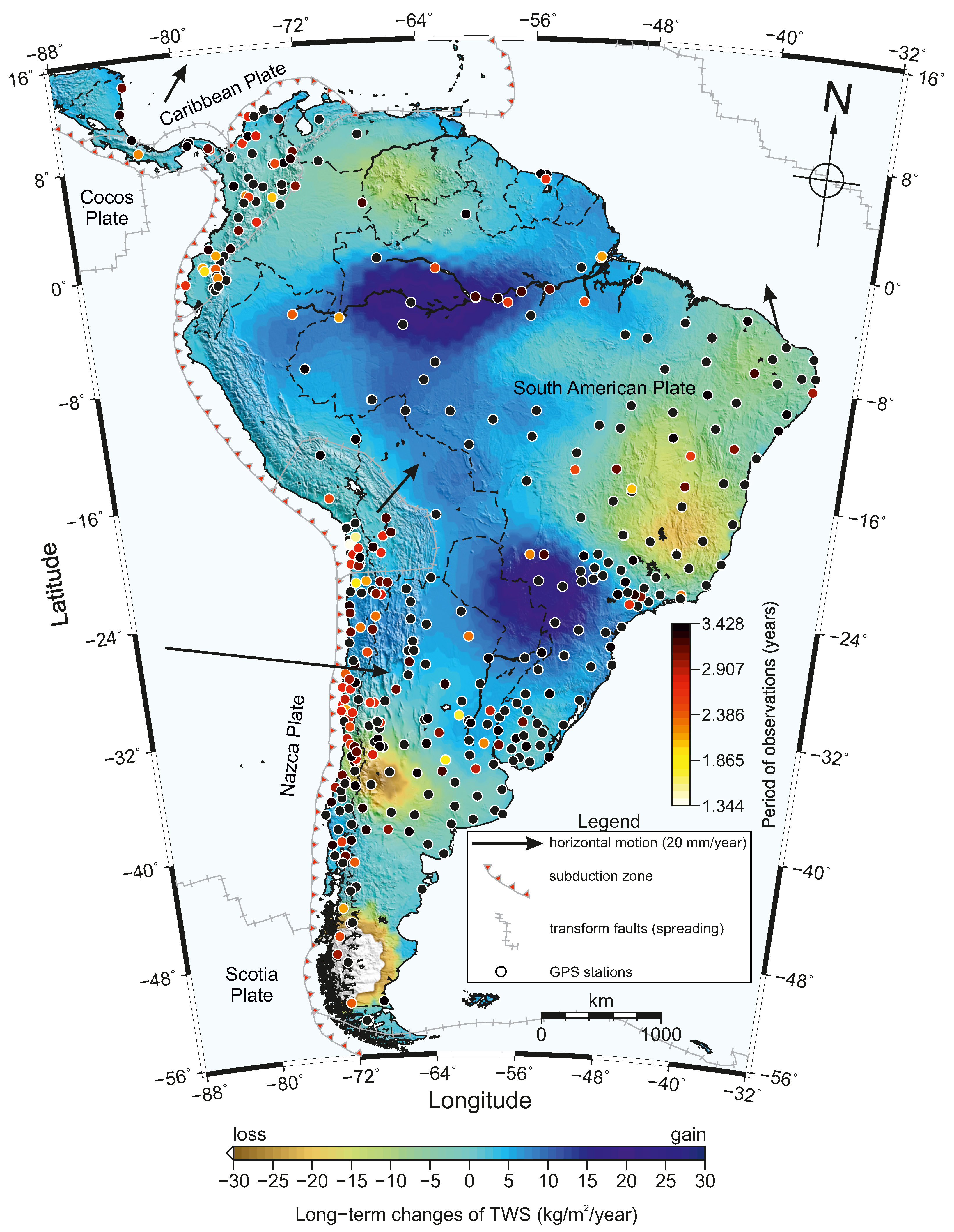
2. Study Area
2.1. Hydrology
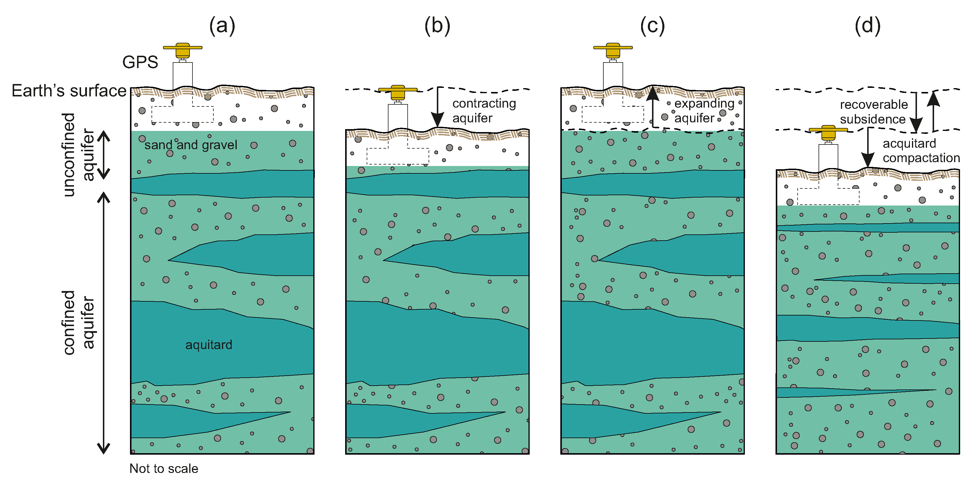
2.2. Geodynamics
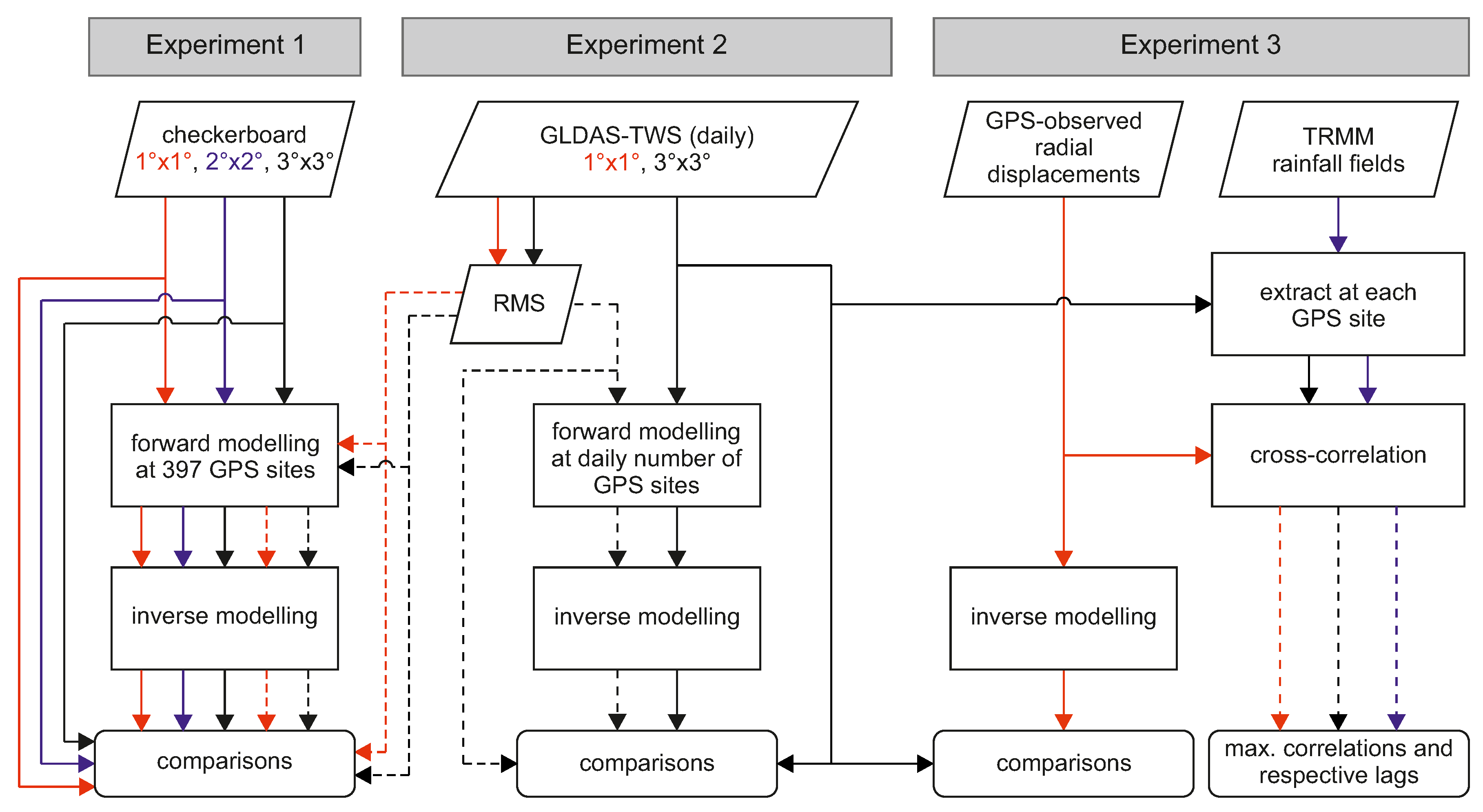
3. Material and Methods
3.1. Datasets
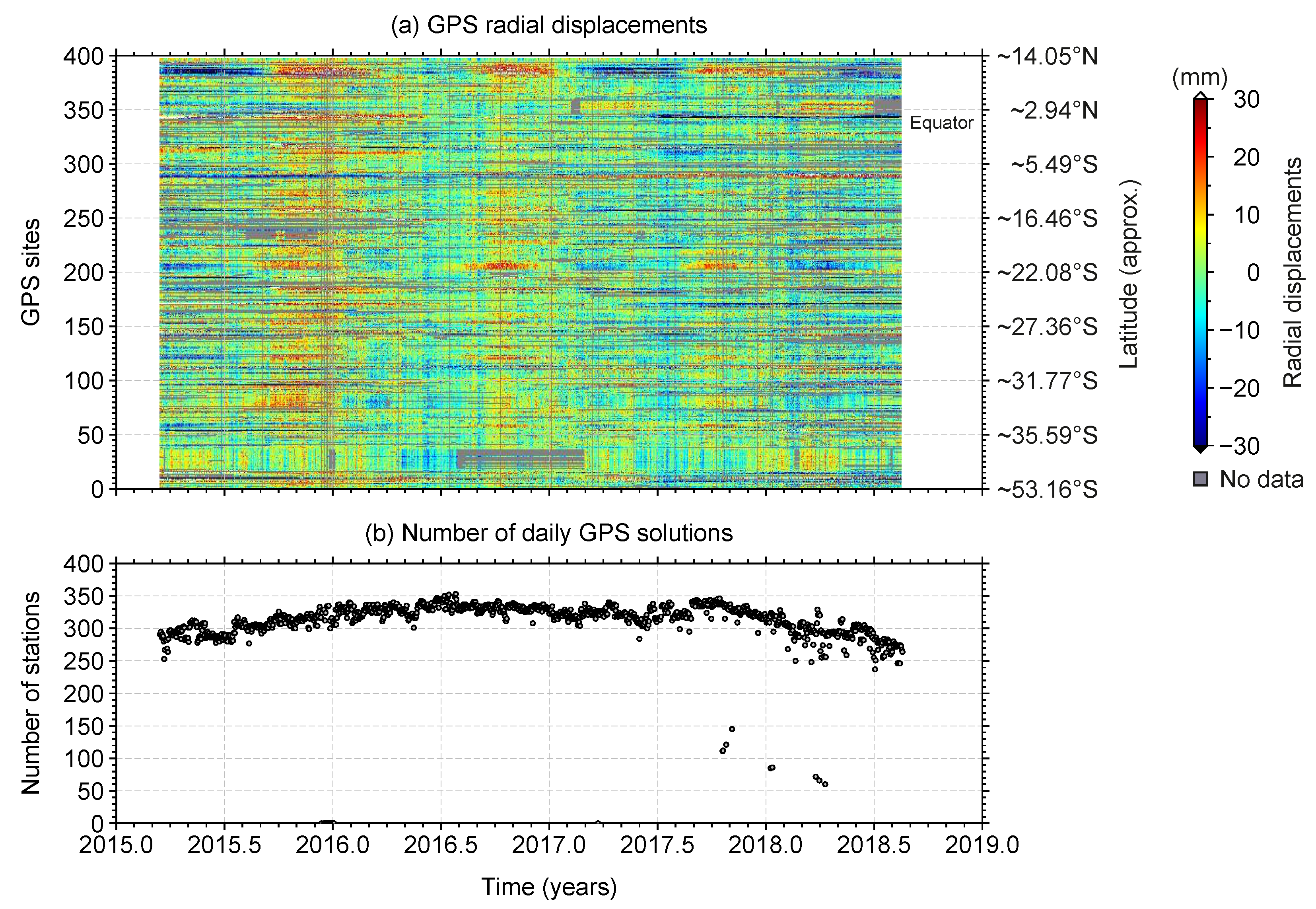
3.1.1. GPS Time Series
3.1.2. Model for Continental Hydrology
3.1.3. TRMM Rainfall Fields
3.1.4. GRACE TWS Solutions
3.2. Methods
3.2.1. Forward Modeling: From Mass Loadings to Radial Displacements
3.2.2. Inverse Modeling: From Radial Displacements to Mass Loadings
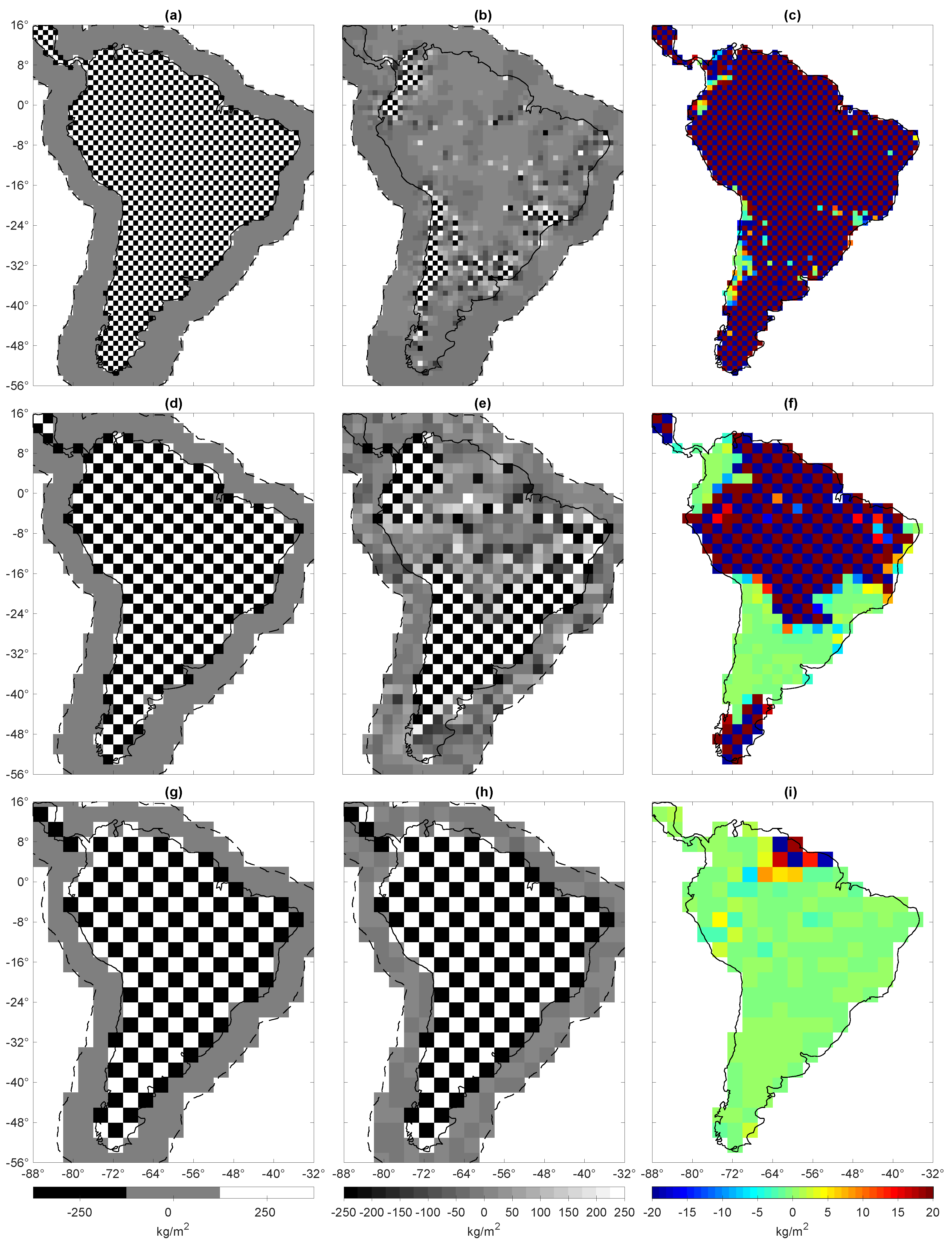
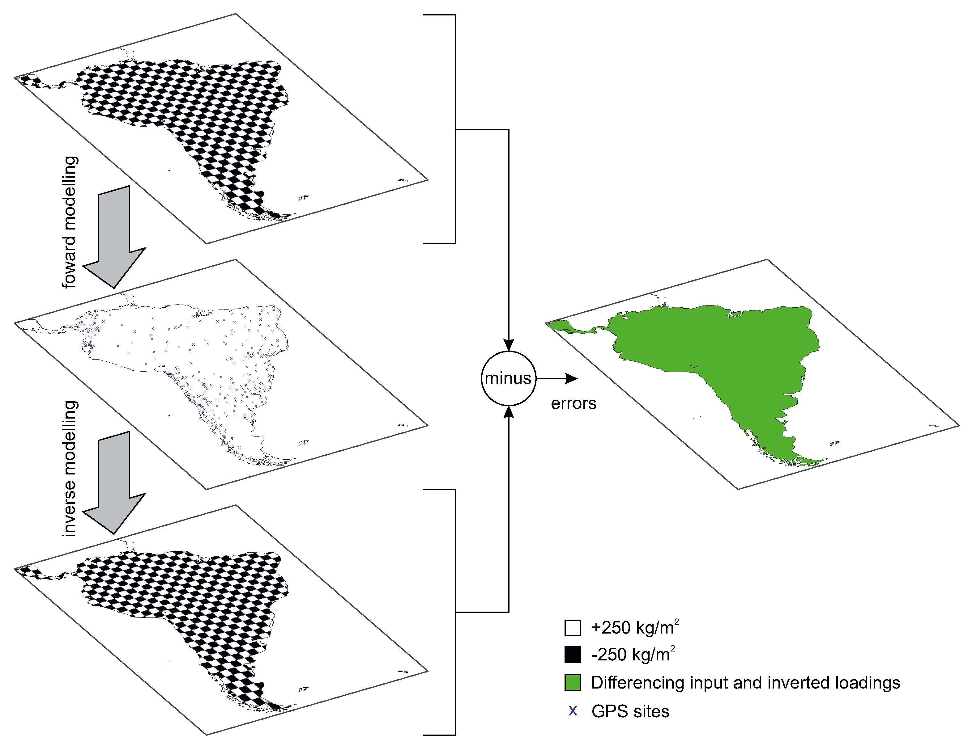
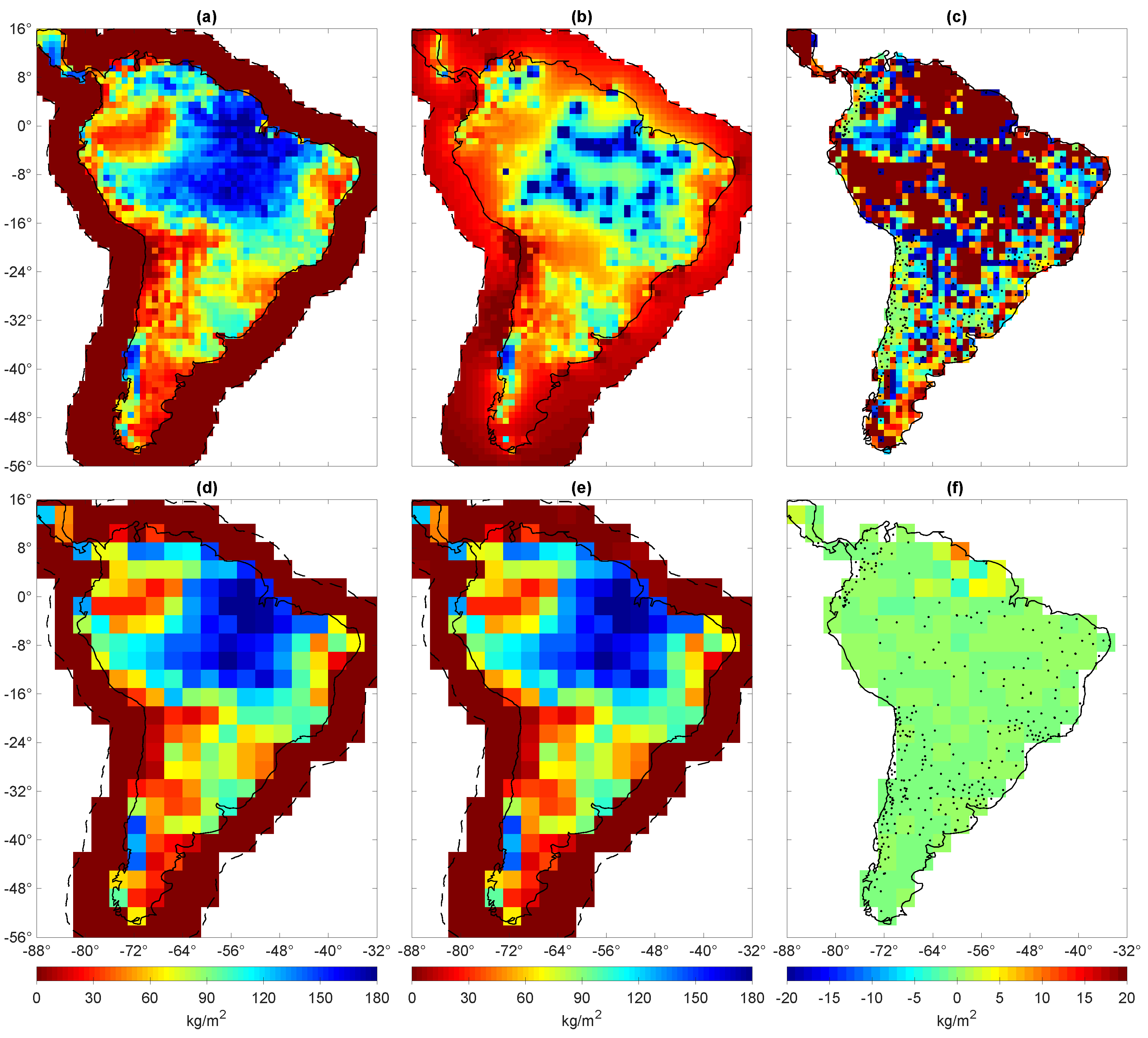
3.2.3. Checkerboard Test: Model Resolution
4. Results
4.1. Experiment 1: What Is the Potential Spatial Resolution of GPS-Imaged TWS over South America?
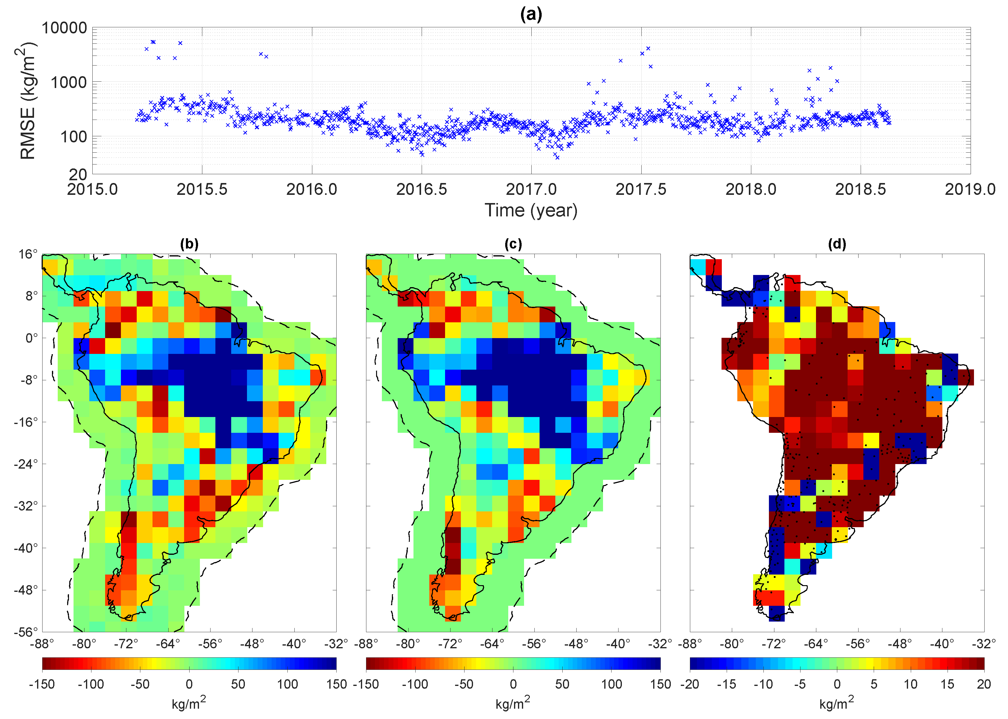
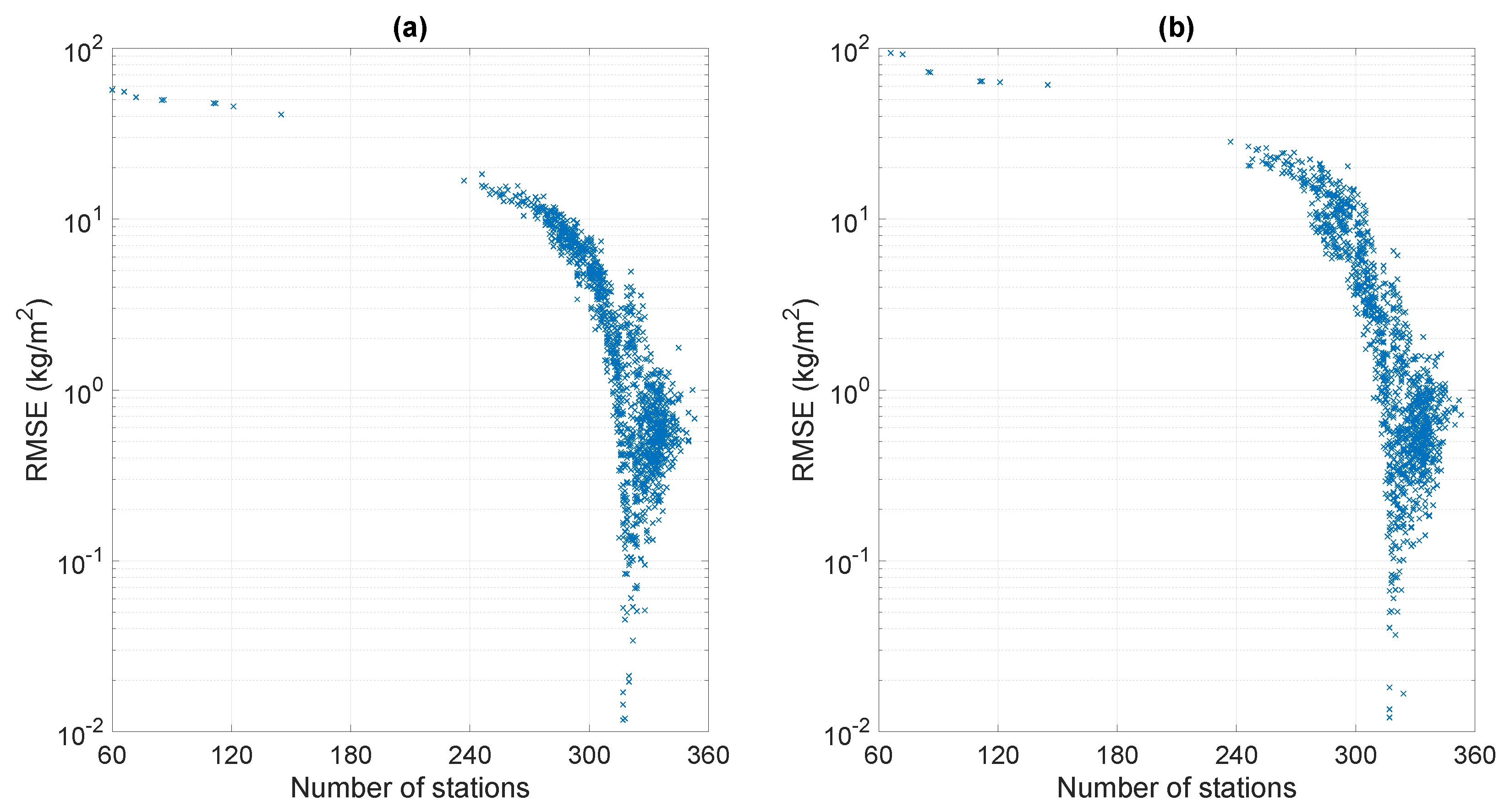
4.2. Experiment 2: How About the Impact of the Varied Number of Daily GPS Data?
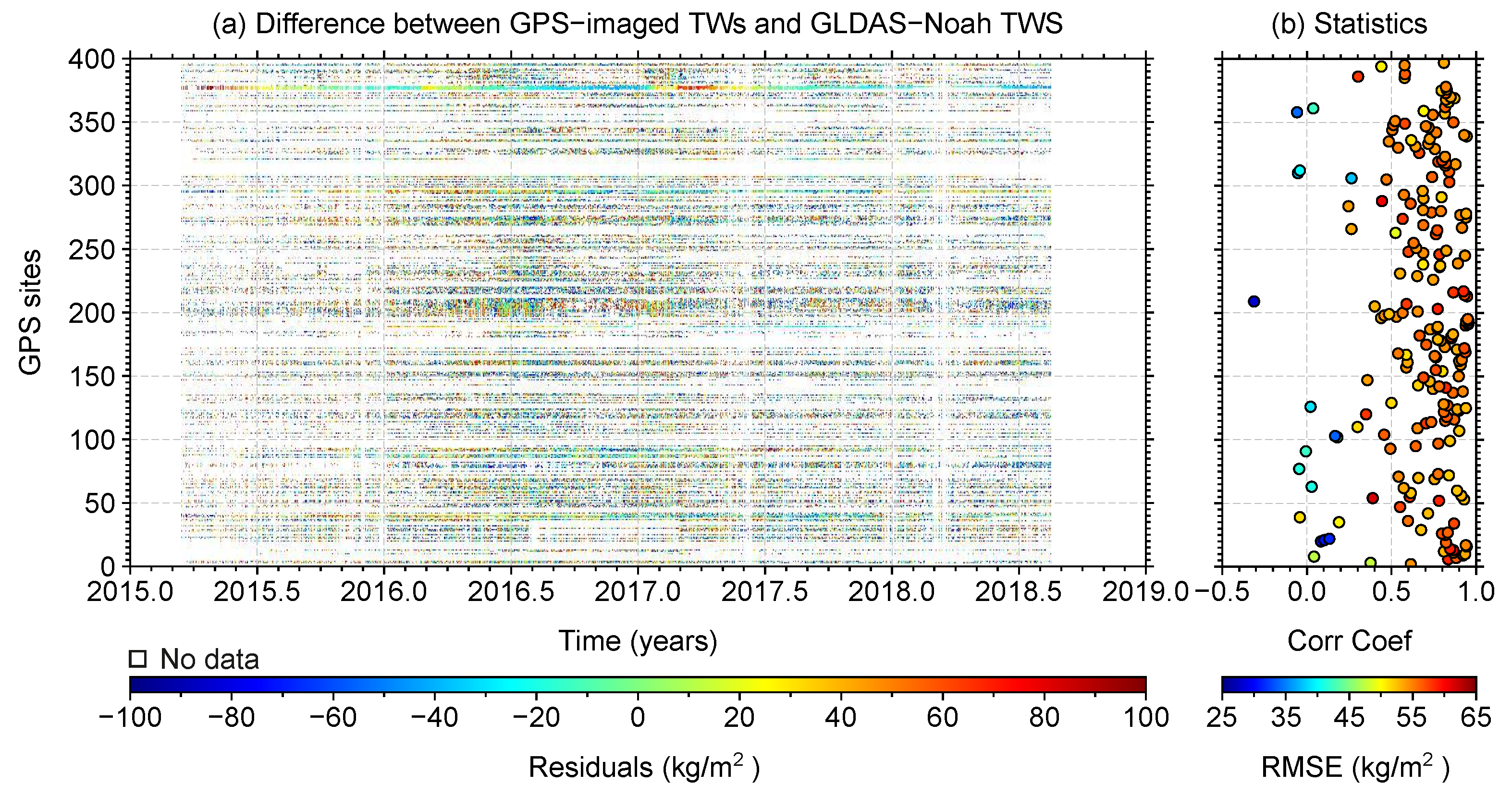
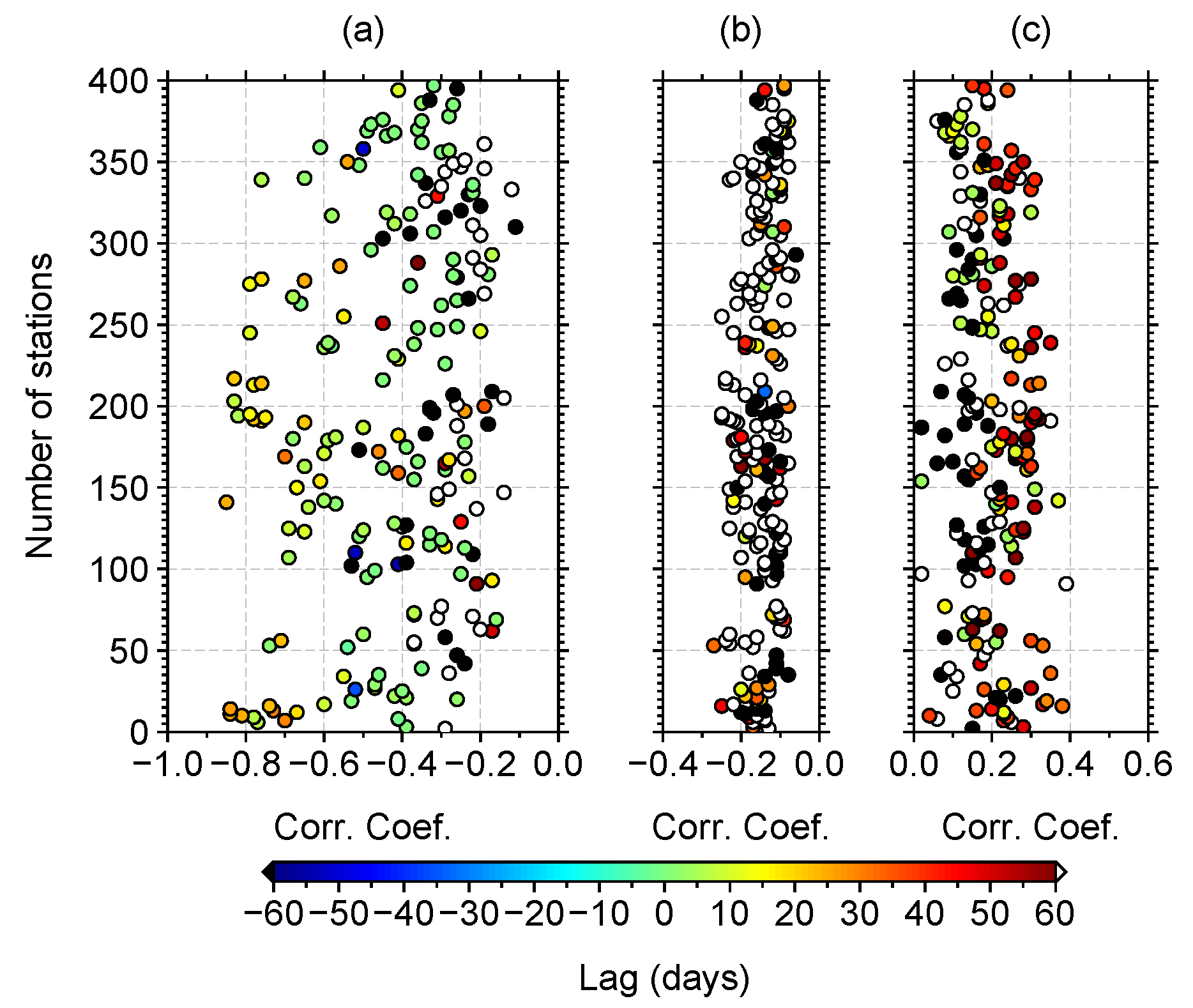
4.3. Experiment 3: What Is the Result of Considering the Actual GPS Data?
5. Discussion
6. Conclusions
Author Contributions
Funding
Acknowledgments
Conflicts of Interest
Appendix A

References
- Cazenave, A.; Chen, J. Time-variable gravity from space and present-day mass redistribution in the Earth system. Earth Planet. Sci. Lett. 2010, 298, 263–274. [Google Scholar] [CrossRef]
- Kusche, J.; Klemann, V.; Bosch, W. Mass distribution and mass transport in the Earth system. J. Geodyn. 2012, 59–60, 1–8. [Google Scholar] [CrossRef]
- Hinderer, J.; Pfeffer, J.; Boucher, M.; Nahmani, S.; Linage, C.; Boy, J.P.; Genthon, P.; Seguis, L.; Favreau, G.; Bock, O.; et al. Land Water Storage Changes from Ground and Space Geodesy: First Results from the GHYRAF (Gravity and Hydrology in Africa) Experiment. Pure Appl. Geophys. 2011, 169, 1391–1410. [Google Scholar] [CrossRef]
- Jacob, T.; Bayer, R.; Chery, J.; Jourde, H.; Moigne, N.L.; Boy, J.P.; Hinderer, J.; Luck, B.; Brunet, P. Absolute gravity monitoring of water storage variation in a karst aquifer on the larzac plateau (Southern France). J. Hydrol. 2008, 359, 105–117. [Google Scholar] [CrossRef]
- Kroner, C.; Jahr, T.; Naujoks, M.; Weise, A. Hydrological signals in gravity—Foe or friend. In Dynamic Planet; Tregoning, P., Rizos, C., Eds.; Springer: Berlin/Heidelberg, Germany, 2007; pp. 504–510. [Google Scholar]
- Hasan, S.; Troch, P.A.; Boll, J.; Kroner, C. Modeling the Hydrological Effect on Local Gravity at Moxa, Germany. J. Hydrometeorol. 2006, 7, 346–354. [Google Scholar] [CrossRef] [Green Version]
- Mäkinen, J.; Tattari, S. Soil moisture and groundwater: Two sources of gravity variations. Bur. Gravim. Int. 1998, 62, 103–110. [Google Scholar]
- Naujoks, M.; Weise, A.; Kroner, C.; Jahr, T. Detection of small hydrological variations in gravity by repeated observations with relative gravimeters. J. Geod. 2008, 82, 543–553. [Google Scholar] [CrossRef]
- Müller, J.; Dirkx, D.; Kopeikin, S.M.; Lion, G.; Panet, I.; Petit, G.; Visser, P.N. High Performance Clocks and Gravity Field Determination. Space Sci. Rev. 2018, 214, 1–31. [Google Scholar] [CrossRef]
- Tapley, B.D.; Bettadpur, S.; Ries, J.C.; Thompson, P.F.; Watkins, M.M. GRACE measurements of mass variability in the Earth system. Science 2004, 305, 503–505. [Google Scholar] [CrossRef]
- National Aeronautics and Space Administration. GRACE-FO: Gravity Recovery and Climate Experiment Follow-On. Available online: https://gracefo.jpl.nasa.gov/resources/38/grace-fo-fact-sheet/ (accessed on 19 January 2019).
- Ouellette, K.J.; de Linage, C.; Famiglietti, J.S. Estimating snow water equivalent from GPS vertical site-position observations in the western United States. Water Resour. Res. 2013, 49, 2508–2518. [Google Scholar] [CrossRef] [Green Version]
- Argus, D.F.; Fu, Y.; Landerer, F.W. Seasonal variation in total water storage in California inferred from GPS observations of vertical land motion. Geophys. Res. Lett. 2014, 41, 1971–1980. [Google Scholar] [CrossRef] [Green Version]
- Borsa, A.A.; Agnew, D.C.; Cayan, D.R. Ongoing drought-induced uplift in the western United States. Science 2014, 345, 1587–1590. [Google Scholar] [CrossRef]
- Fu, Y.; Argus, D.F.; Landerer, F.W. GPS as an independent measurement to estimate terrestrial water storage variations in Washington and Oregon. J. Geophys. Res. Solid Earth 2015, 120, 552–566. [Google Scholar] [CrossRef] [Green Version]
- Enzminger, T.L.; Small, E.E.; Borsa, A.A. Accuracy of Snow Water Equivalent Estimated From GPS Vertical Displacements: A Synthetic Loading Case Study for Western U.S. Mountains. Water Resour. Res. 2018, 54, 581–599. [Google Scholar] [CrossRef]
- Jin, S.; Zhang, T. Terrestrial Water Storage Anomalies Associated with Drought in Southwestern USA from GPS Observations. Surv. Geophys. 2016, 37, 1139–1156. [Google Scholar] [CrossRef]
- Zhang, B.; Yao, Y.; Fok, H.S.; Hu, Y.; Chen, Q. Potential seasonal terrestrial water storage monitoring from GPS vertical displacements: A case study in the lower three-rivers headwater region, China. Sensors 2016, 16, 1526. [Google Scholar] [CrossRef]
- Chew, C.C.; Small, E.E. Terrestrial water storage response to the 2012 drought estimated from GPS vertical position anomalies. Geophys. Res. Lett. 2014, 41, 6145–6151. [Google Scholar] [CrossRef] [Green Version]
- Jiang, W.; Yuan, P.; Chen, H.; Cai, J.; Li, Z.; Chao, N.; Sneeuw, N. Annual variations of monsoon and drought detected by GPS: A case study in Yunnan, China. Sci. Rep. 2017, 7, 5874. [Google Scholar] [CrossRef]
- Ferreira, V.; Montecino, H.; Ndehedehe, C.; Heck, B.; Gong, Z.; de Freitas, S.; Westerhaus, M. Space-based observations of crustal deflections for drought characterization in Brazil. Sci. Total Environ. 2018, 644, 256–273. [Google Scholar] [CrossRef]
- Azmi, M.; Rüdiger, C.; Walker, J.P. A data fusion-based drought index. Water Resour. Res. 2016, 52, 2222–2239. [Google Scholar] [CrossRef]
- Birhanu, Y.; Bendick, R. Monsoonal loading in Ethiopia and Eritrea from vertical GPS displacement time series. J. Geophys. Res. Solid Earth 2015, 120, 7231–7238. [Google Scholar] [CrossRef]
- Moreira, D.M.; Calmant, S.; Perosanz, F.; Xavier, L.; Rotunno Filho, O.C.; Seyler, F.; Monteiro, A.C. Comparisons of observed and modeled elastic responses to hydrological loading in the Amazon basin. Geophys. Res. Lett. 2016, 43, 9604–9610. [Google Scholar] [CrossRef]
- Orme, A.R. The Tectonic Framework of South America; Oxford Regional Environments; Oxford University Press: Oxford, UK, 2007; Chapter 1; pp. 3–22. [Google Scholar]
- Orme, A.R. Tectonism, Climate, and Landscape Change; Oxford Regional Environments; Oxford University Press: Oxford, UK, 2007; Chapter 2; pp. 23–44. [Google Scholar]
- de Linage, C.; Kim, H.; Famiglietti, J.S.; Yu, J.Y. Impact of Pacific and Atlantic sea surface temperatures on interannual and decadal variations of GRACE land water storage in tropical South America. J. Geophys. Res. Atmos. 2013, 118, 10,811–10,829. [Google Scholar] [CrossRef] [Green Version]
- Buytaert, W.; Breuer, L. Water resources in South America: Sources and supply, pollutants and perspectives. In Understanding Freshwater Quality Problems in a Changing World; International Association of Hydrological Sciences: London, UK, 2013; Volume 359, pp. 106–113. [Google Scholar]
- Dunne, T.; Mertes, L.A.K. Rivers; Oxford Regional Environments; Oxford University Press: Oxford, UK, 2007; Chapter 5; pp. 76–90. [Google Scholar]
- Zarfl, C.; Lumsdon, A.E.; Berlekamp, J.; Tydecks, L.; Tockner, K. A global boom in hydropower dam construction. Aquat. Sci. 2014, 77, 161–170. [Google Scholar] [CrossRef]
- Veblen, T.T.; Young, K.R.; Orme, A.R. Future Environments of South America; Oxford Regional Environments; Oxford University Press: Oxford, UK, 2007; Chapter 21; pp. 340–352. [Google Scholar]
- Reboućas, A.d.C. Groundwater resources in South America. Episodes 1999, 3, 232–237. [Google Scholar]
- Da Silva, G.C.; Bocanegra, E.; Montenegro, S.; Custodio, E.; Manzano, M. State of knowledge of coastal aquifer management in South America. Hydrogeol. J. 2009, 18, 261–267. [Google Scholar] [CrossRef] [Green Version]
- Siebert, S.; Burke, J.; Faures, J.M.; Frenken, K.; Hoogeveen, J.; Döll, P.; Portmann, F.T. Groundwater use for irrigation—A global inventory. Hydrol. Earth Syst. Sci. 2010, 14, 1863–1880. [Google Scholar] [CrossRef]
- Morris, B.L.; Lawrence, A.R.L.; Chilton, P.J.C.; Adams, B.; Calow, R.C.; Klinck, B.A. Groundwater and Its Susceptibility to Degradation: A Global Assessment of the Problem and Options for Management; Technical Report RS. 03-3; United Nations Environment Programme: Nairobi, Kenya, 2003. [Google Scholar]
- Rodell, M.; Famiglietti, J.S.; Wiese, D.N.; Reager, J.T.; Beaudoing, H.K.; Landerer, F.W.; Lo, M.H. Emerging trends in global freshwater availability. Nature 2018, 557, 651–659. [Google Scholar] [CrossRef]
- Frappart, F.; Papa, F.; Santos Da Silva, J.; Ramillien, G.; Prigent, C.; Seyler, F.; Calmant, S. Surface freshwater storage and dynamics in the Amazon basin during the 2005 exceptional drought. Environ. Res. Lett. 2012, 7. [Google Scholar] [CrossRef]
- Frappart, F.; Papa, F.; Malbeteau, Y.; León, J.G.; Ramillien, G.; Prigent, C.; Seoane, L.; Seyler, F.; Calmant, S. Surface freshwater storage variations in the Orinoco floodplains using multi-satellite observations. Remote Sens. 2015, 7, 89–110. [Google Scholar] [CrossRef]
- Alves, L.M.; Camargo, H.; Nobre, C.A.; Oyama, M.D.; Marengo, J.A.; Tomasella, J.; Sampaio de Oliveira, G.; Brown, I.F.; de Oliveira, R. The Drought of Amazonia in 2005. J. Clim. 2008, 21, 495–516. [Google Scholar] [CrossRef]
- Getirana, A. Extreme Water Deficit in Brazil Detected from Space. J. Hydrometeorol. 2016, 17, 591–599. [Google Scholar] [CrossRef]
- Sun, T.; Ferreira, V.; He, X.; Andam-Akorful, S. Water Availability of São Francisco River Basin Based on a Space-Borne Geodetic Sensor. Water 2016, 8, 213. [Google Scholar] [CrossRef]
- Trotman, A.R.; Farrell, D.A. Drought Impacts and Early Warning in the Caribbean: The Drought of 2009–2010. Available online: https://www.wmo.int/pages/prog/drr/events/Barbados/Pres/4-CIMH-Drought.pdf (accessed on 27 January 2019).
- Willis, M.J.; Melkonian, A.K.; Pritchard, M.E.; Rivera, A. Ice loss from the Southern Patagonian Ice Field, South America, between 2000 and 2012. Geophys. Res. Lett. 2012, 39, L17501. [Google Scholar] [CrossRef]
- Han, S.C.; Sauber, J.; Luthcke, S. Regional gravity decrease after the 2010 Maule (Chile) earthquake indicates large-scale mass redistribution. Geophys. Res. Lett. 2010, 37, 1–5. [Google Scholar] [CrossRef]
- Vigny, C.; Socquet, A.; Peyrat, S.; Ruegg, J.C.; Métois, M.; Madariaga, R.; Morvan, S.; Lancieri, M.; Lacassin, R.; Campos, J.; et al. The 2010 Mw 8.8 Maule megathrust earthquake of Central Chile, monitored by GPS. Science 2011, 332, 1417–1421. [Google Scholar] [CrossRef] [PubMed]
- Sánchez, L.; Drewes, H. Crustal deformation and surface kinematics after the 2010 earthquakes in Latin America. J. Geodyn. 2016, 102, 1–23. [Google Scholar] [CrossRef]
- Biggs, J.; Ebmeier, S.K.; Aspinall, W.P.; Lu, Z.; Pritchard, M.E.; Sparks, R.S.J.; Mather, T.A. Global link between deformation and volcanic eruption quantified by satellite imagery. Nat. Commun. 2014, 5, 3471. [Google Scholar] [CrossRef] [Green Version]
- Reath, K.; Pritchard, M.; Poland, M.; Delgado, F.; Carn, S.; Coppola, D.; Andrews, B.; Ebmeier, S.K.; Rumpf, E.; Henderson, S.; et al. Thermal, Deformation, and Degassing Remote Sensing Time Series (CE 2000-2017) at the 47 most Active Volcanoes in Latin America: Implications for Volcanic Systems. J. Geophys. Res. Solid Earth 2019, 124, 195–218. [Google Scholar] [CrossRef]
- Pritchard, M.E.; Jay, J.A.; Aron, F.; Henderson, S.T.; Lara, L.E. Subsidence at southern Andes volcanoes induced by the 2010 Maule, Chile earthquake. Nat. Geosci. 2013, 6, 632–636. [Google Scholar] [CrossRef]
- Pritchard, M.E.; Simons, M. An InSAR-based survey of volcanic deformation in the central Andes. Geochem. Geophys. Geosyst. 2004, 5. [Google Scholar] [CrossRef] [Green Version]
- Save, H.; Bettadpur, S.; Tapley, B.D. High-resolution CSR GRACE RL05 mascons. J. Geophys. Res. Solid Earth 2016, 121, 7547–7569. [Google Scholar] [CrossRef]
- Bird, P. An updated digital model of plate boundaries. Geochem. Geophys. Geosyst. 2003, 4. [Google Scholar] [CrossRef] [Green Version]
- Ingebritsen, S.E.; Sanford, W.E. Groundwater in Geologic Processes, 1st ed.; Cambridge University Press: Cambridge, UK, 1998. [Google Scholar]
- Mohr, C.H.; Manga, M.; Wang, C.Y.; Korup, O. Regional changes in streamflow after a megathrust earthquake. Earth Planet. Sci. Lett. 2017, 458, 418–428. [Google Scholar] [CrossRef]
- Verdugo, R.; Villalobos, F.; Yasuda, S.; Konagai, K.; Sugano, T.; Okamura, M.; Tobita, T.; Torres, A. Description and analysis of geotechnical aspects associated to the 2010 Chile earthquake. Obras y Proyectos 2010, 8, 27–33. [Google Scholar]
- Montecino, H.D.; de Freitas, S.R.; Báez, J.C.; Ferreira, V.G. Effects on Chilean Vertical Reference Frame due to the Maule Earthquake co-seismic and post-seismic effects. J. Geodyn. 2017, 112, 22–30. [Google Scholar] [CrossRef]
- Dill, R.; Dobslaw, H. Numerical simulations of global-scale high-resolution hydrological crustal deformations. J. Geophys. Res. Solid Earth 2013, 118, 5008–5017. [Google Scholar] [CrossRef] [Green Version]
- Kennett, B.L.N.; Engdahl, E.R.; Buland, R. Constraints on seismic velocities in the Earth from traveltimes. Geophys. J. Int. 1995, 122, 108–124. [Google Scholar] [CrossRef] [Green Version]
- Bevis, M.; Brown, A. Trajectory models and reference frames for crustal motion geodesy. J. Geod. 2014, 88, 283–311. [Google Scholar] [CrossRef] [Green Version]
- Rodell, M.; Houser, P.R.; Jambor, U.; Gottschalck, J.; Mitchell, K.; Meng, C.J.; Arsenault, K.; Cosgrove, B.; Radakovich, J.; Bosilovich, M.; et al. The Global Land Data Assimilation System. Bull. Am. Meteorol. Soc. 2004, 85, 381–394. [Google Scholar] [CrossRef] [Green Version]
- Hiroko, B.; Rodell, M.; NASA/GSFC/HSL. GLDAS Noah Land Surface Model L4 3 hourly 0.25 × 0.25 degree V2.1. Goddard Earth Sciences Data and Information Services Center (GES DISC). 2016. Available online: https://disc.gsfc.nasa.gov/datasets/GLDAS_NOAH025_3H_V2.1/summary?keywords=GLDAS (accessed on 25 December 2018).
- Eriksson, D.; MacMillan, D.S. Continental hydrology loading observed by VLBI measurements. J. Geod. 2014, 88, 675–690. [Google Scholar] [CrossRef]
- Huffman, G.J.; Bolvin, D.T.; Nelkin, E.J.; Wolff, D.B.; Adler, R.F.; Gu, G.; Hong, Y.; Bowman, K.P.; Stocker, E.F. The TRMM Multisatellite Precipitation Analysis (TMPA): Quasi-Global, Multiyear, Combined-Sensor Precipitation Estimates at Fine Scales. J. Hydrometeorol. 2007, 8, 38–55. [Google Scholar] [CrossRef]
- Scanlon, B.R.; Zhang, Z.; Save, H.; Sun, A.Y.; Müller Schmied, H.; van Beek, L.P.H.; Wiese, D.N.; Wada, Y.; Long, D.; Reedy, R.C.; et al. Global models underestimate large decadal declining and rising water storage trends relative to GRACE satellite data. Proc. Natl. Acad. Sci. USA 2018, 115, E1080–E1089. [Google Scholar] [CrossRef] [PubMed] [Green Version]
- Lambeck, K. Geophysical Geodesy: The Slow Deformations of the Earth; Oxford University Press: Oxford, UK, 1988. [Google Scholar]
- Ray, R.D.; Sanchez, B.V. Radial Deformation of the Earth by Oceanic Tidal Loading; 1989. Available online: https://denali.gsfc.nasa.gov/personal_pages/ray/MiscPubs/19890016938_1989016938.pdf (accessed on 21 July 2018).
- Farrell, W.E. Deformation of the Earth by surface loads. Rev. Geophys. 1972, 10, 761–797. [Google Scholar] [CrossRef]
- Wang, H.; Xiang, L.; Jia, L.; Jiang, L.; Wang, Z.; Hu, B.; Gao, P. Load Love numbers and Green’s functions for elastic Earth models PREM, iasp91, ak135, and modified models with refined crustal structure from Crust 2.0. Comput. Geosci. 2012, 49, 190–199. [Google Scholar] [CrossRef]
- Galloway, D.; Jones, D.R. Land Subsidence in the United States; Technical Report Circular 1182; U.S. Geological Survey: Reston, VA, USA, 1999.
- Bouman, J. Quality of Regularization Methods; Technical Report 98.2; TU Delft, DEOS: Delft, The Netherlands, 2010. [Google Scholar]
- Aster, R.C.; Borchers, B.; Thurber, C.H. Parameter Estimation and Inverse Problems, 1st ed.; Elsevier: Amsterdam, The Netherlands, 2005; p. 316. [Google Scholar]
- Golub, G.H.; Heath, M.; Wahba, G. Generalized Cross-Validation as a Method for Choosing a Good Ridge Parameter. Technometrics 1979, 21, 215–223. [Google Scholar] [CrossRef]
- Wahba, G. Estimating the Smoothing Parameter. In Spline Models for Observational Data; Wahba, G., Ed.; CBMS-NSF Regional Conference Series in Applied Mathematics; Society for Industrial and Applied Mathematics (SIAM): Montpelier, Vermont, 1990; Chapter 4; pp. 45–65. [Google Scholar] [CrossRef]
- Hansen, P.C. Analysis of Discrete Ill-Posed Problems by Means of the L–Curve. SIAM Rev. 2005, 34, 561–580. [Google Scholar] [CrossRef]
- Page, M.T.; Custódio, S.; Archuleta, R.J.; Carlson, J.M. Constraining earthquake source inversions with GPS data: 1. Resolution-based removal of artifacts. J. Geophys. Res. Solid Earth 2009, 114, 1–13. [Google Scholar] [CrossRef]
- Lévěque, J.J.; Rivera, L.; Wittlinger, G. On the use of the checker-board test to assess the resolution of tomographic inversions. Geophys. J. Int. 1993, 115, 313–318. [Google Scholar] [CrossRef] [Green Version]
- de Luna, R.M.R.; Garnés, S.J.d.A.; Cabral, J.J.d.S.P.; dos Santos, S.M. Groundwater overexploitation and soil subsidence monitoring on Recife plain (Brazil). Nat. Hazards 2017, 86, 1363–1376. [Google Scholar] [CrossRef]
- Coelho, V.H.R.; Bertrand, G.F.; Montenegro, S.M.; Paiva, A.L.; Almeida, C.N.; Galvão, C.O.; Barbosa, L.R.; Batista, L.F.; Ferreira, E.L. Piezometric level and electrical conductivity spatiotemporal monitoring as an instrument to design further managed aquifer recharge strategies in a complex estuarial system under anthropogenic pressure. J. Environ. Manag. 2018, 209, 426–439. [Google Scholar] [CrossRef] [PubMed]


| Synthetic Experiments | |||||||||
|---|---|---|---|---|---|---|---|---|---|
| Summary | Checkerboard | GLDAS-TWS | Daily GPS Data | ||||||
| RMS of TWS | Daily TWS | ||||||||
| Resolution | site | ||||||||
| No. of observ. | 397 | 397 | 397 | 397 | 397 | varied | varied | varied | - |
| RMSE (kg/m) | 233.88 | 163.00 | 3.90 | 38.34 | 1.10 | 3.29 | 4.50 | 80.49 | 53.48 |
| Bias (kg/m) | −0.85 | −0.76 | −0.02 | 12.86 | 0.13 | 0.50 | 0.11 | 3.36 | −0.29 |
| Is it feasible? | ✗ | ✗ | ✓ | ✗ | ✓ | ✓ | ✓ | ✓ * | ✓ |
© 2019 by the authors. Licensee MDPI, Basel, Switzerland. This article is an open access article distributed under the terms and conditions of the Creative Commons Attribution (CC BY) license (http://creativecommons.org/licenses/by/4.0/).
Share and Cite
Ferreira, V.G.; Ndehedehe, C.E.; Montecino, H.C.; Yong, B.; Yuan, P.; Abdalla, A.; Mohammed, A.S. Prospects for Imaging Terrestrial Water Storage in South America Using Daily GPS Observations. Remote Sens. 2019, 11, 679. https://doi.org/10.3390/rs11060679
Ferreira VG, Ndehedehe CE, Montecino HC, Yong B, Yuan P, Abdalla A, Mohammed AS. Prospects for Imaging Terrestrial Water Storage in South America Using Daily GPS Observations. Remote Sensing. 2019; 11(6):679. https://doi.org/10.3390/rs11060679
Chicago/Turabian StyleFerreira, Vagner G., Christopher E. Ndehedehe, Henry C. Montecino, Bin Yong, Peng Yuan, Ahmed Abdalla, and Abubakar S. Mohammed. 2019. "Prospects for Imaging Terrestrial Water Storage in South America Using Daily GPS Observations" Remote Sensing 11, no. 6: 679. https://doi.org/10.3390/rs11060679