Abstract
The Visible Infrared Imaging Radiometer Suite (VIIRS) on the Suomi National Polar-orbiting Partnership (SNPP) and National Oceanic and Atmospheric Administration (NOAA)-20 has been providing a large amount of global ocean color data, which are critical for monitoring and understanding of ocean optical, biological, and ecological processes and phenomena. However, VIIRS-derived daily ocean color images on either SNPP or NOAA-20 have some limitations in ocean coverage due to its swath width, high sensor-zenith angle, high sun glint, and cloud, etc. Merging VIIRS ocean color products derived from the SNPP and NOAA-20 significantly increases the spatial coverage of daily images. The two VIIRS sensors on the SNPP and NOAA-20 have similar sensor characteristics, and global ocean color products are generated using the same Multi-Sensor Level-1 to Level-2 (MSL12) ocean color data processing system. Therefore, the merged VIIRS ocean color data from the two sensors have high data quality with consistent statistical property and accuracy globally. Merging VIIRS SNPP and NOAA-20 ocean color data almost removes the gaps of missing pixels due to high sensor-zenith angles and high sun glint contamination, and also significantly reduces the gaps due to cloud cover. However, there are still gaps of missing pixels in the merged ocean color data. In this study, the Data Interpolating Empirical Orthogonal Functions (DINEOF) are applied on the merged VIIRS SNPP/NOAA-20 global Level-3 ocean color data to completely reconstruct the missing pixels. Specifically, DINEOF is applied to 30 days of daily merged global Level-3 chlorophyll-a (Chl-a) data of 9-km spatial resolution from 19 June to 18 July 2018. To quantitatively evaluate the accuracy of the DINEOF reconstructed data, a set of valid pixels are intentionally treated as “missing pixels”, so that reconstructed data can be compared with the original data. Results show that mean ratios of the reconstructed/original are 1.012, 1.012, 1.015, and 0.997 for global ocean, oligotrophic waters, deep waters, and coastal and inland waters, respectively. The corresponding standard deviation (SD) of the ratios are 0.200, 0.164, 0.182, and 0.287, respectively. Gap-filled daily Chl-a images reveal many large-scale and meso-scale ocean features that are invisible in the original SNPP or NOAA-20 Chl-a images. It is also demonstrated that the gap-filled data based on the merged products show more details in the dynamic ocean features than those based on SNPP or NOAA-20 alone.
1. Introduction
Ocean color data are critical for monitoring and understanding of water optical, biological, and ecological processes and phenomena, and it is also an important source of input data for physical and biogeochemical ocean models [1]. Since the launch of the Visible Infrared Imaging Radiometer Suite (VIIRS) on the Suomi National Polar-Orbiting Partnership (SNPP) [2,3] in October 2011, ocean color products derived from VIIRS-SNPP have been routinely produced globally [3,4]. On 18 November 2017, the follow-up VIIRS sensor housed in the National Oceanic and Atmospheric Administration (NOAA)-20 satellite was launched as the first of four sensors in the Joint Polar Satellite System (JPSS) satellite series, and global ocean color data from NOAA-20 are also being routinely produced. For both SNPP and NOAA-20, chlorophyll-a (Chl-a) concentration [5,6,7], normalized water-leaving radiance spectra nLw(λ) [8,9], including new nLw(λ) data using VIIRS imaging bands [10], and water diffuse attenuation coefficient at the wavelength of 490 nm Kd(490) and at the domain of photosynthetically available radiation (PAR) Kd(PAR) [11,12], are all generated as standard VIIRS ocean color products. Some experimental products such as inherent optical properties (IOPs) [13,14], and a newly added quality assurance (QA) score product for measuring data quality [15] are also included for evaluation. In addition, to improve ocean color data quality over turbid coastal and inland waters [16,17,18], the shortwave infrared (SWIR)-based and near-infrared (NIR)-SWIR combined atmospheric correction algorithms have been used to routinely produce global VIIRS ocean color products for both SNPP and NOAA-20 [19,20]. Furthermore, VIIRS ocean color data processing algorithms have been significantly improved, including improved sensor on-orbit calibration using both solar and lunar approaches [21,22]. However, for either VIIRS-SNPP or VIIRS-NOAA-20, there are always missing pixels in the VIIRS-measured ocean color data imageries due to cloud cover and various other reasons, e.g., strong sun glint contamination, dust storms, very large solar- and sensor-zenith angles, etc. It is certainly useful to fill the gap of missing pixels before being used as input for ocean models and for various other applications.
As a follow-up VIIRS instrument, VIIRS-NOAA-20 is essentially built the same as VIIRS-SNPP. Therefore, the sensor characteristics of the two instruments are very similar. Both SNPP and NOAA-20 operate at the 824-km sun-synchronous polar orbit, which crosses the equator at about 13:30 local time. There is about a 50-minute delay between the paths of NOAA-20 and SNPP, which makes the NOAA-20’s path running through the middle of two adjacent SNPP paths, and vice versa. The overlap of the spatial coverages of the two sensors automatically fills each other’s gaps caused by high sensor-zenith angles and high sun glint contamination, and it significantly reduces the missing pixels in the merged images. In addition, ocean color products from SNPP and NOAA-20 have the same spatial and temporal resolution, and are processed with the same software package, i.e., the Multi-Sensor Level-1 to Level-2 (MSL12) ocean color data processing system [3]. Therefore, the statistics of their ocean color products are very close to each other, and in fact the data can be directly merged without adjustment for matching up each other’s statistical properties. However, there are still lots of missing data in the merged VIIRS SNPP/NOAA-20 products.
To completely fill the gaps of missing pixels in the merged VIIRS SNPP/NOAA-20 ocean color data, the Data Interpolating Empirical Orthogonal Functions (DINEOF) [23,24] method is used in this study to reconstruct the missing data in the ocean color images. The DINEOF exploits the spatio-temporal coherency of the data to infer a value at the missing location and has been successfully adopted in various applications using ocean remote sensing data [25,26,27,28,29,30]. With more and more availability and usage of ocean color data in recent years, the DINEOF method has also been applied to ocean color data from various sensors including the Moderate Resolution Imaging Spectroradiometer (MODIS) [31,32,33], the Spinning Enhanced Visible and Infrared Imager (SEVIRI) onboard Meteosat Second Generation 2 [34], and the Korean Geostationary Ocean Color Imager (GOCI) [35]. Most recently, Liu and Wang [36] used the DINEOF to fill the gaps of missing pixels in VIIRS-SNPP global ocean color data. In that study, the DINEOF is applied to VIIRS-SNPP global Level-3 binned ocean color data of 9-km spatial resolution and the DINEOF reconstructed ocean color data are used to fill the gap of missing data. In particular, daily, 8-day, and monthly VIIRS global Level-3 binned ocean color data, including Chl-a concentration, Kd(490), as well as nLw(λ) at the five VIIRS visible bands are tested and evaluated. Results show that the DINEOF method can successfully reconstruct and gap-fill meso-scale and large-scale spatial ocean features in the global VIIRS Level-3 images, as well as capture the temporal variations of these features.
In this study, the DINEOF method is used to reconstruct and gap-fill a merged VIIRS SNPP/NOAA-20 global daily ocean color product, specifically the Chl-a data. With the reconstructed (gap-filled) VIIRS global daily Chl-a images, ocean features can now be well identified and observed both spatially and temporally. Some examples that demonstrate the advantages and usefulness of the gap-filled VIIRS SNPP/NOAA-20 merged global ocean color products are provided. The DINEOF is also applied to ocean color data from a single sensor, VIIRS-SNPP or VIIRS-NOAA-20, and the gap-filled data based on SNPP or NOAA-20 are compared with those based on the two-sensor merged Chl-a product.
2. Data and Methods
2.1. VIIRS SNPP and NOAA-20 Ocean Color Level-2 and Global Level-3 Data
The MSL12 is the official NOAA VIIRS ocean color data processing system for both SNPP and NOAA-20 (and all other follow-on VIIRS sensors), and it has been used for processing VIIRS data from Sensor Data Records (SDR or Level-1B data) to the Environmental Data Records (EDR or Level-2 data) [3,4]. MSL12 was developed for producing consistent ocean color products using the same ocean color data processing system for multiple satellite ocean color sensors [37,38,39]. In addition to the standard NIR-based atmospheric correction algorithm [8], the current version of MSL12 has been improved to include the SWIR- and NIR-SWIR-based atmospheric correction algorithms [16,19,20], including a recent algorithm improvement using the information from the short blue band, i.e., M1 in Table 1 [40], for improved satellite ocean color data over coastal and inland waters. Indeed, advantages of the SWIR-based ocean color data processing over global highly turbid coastal and inland waters for various applications have been demonstrated in several previous studies [41,42,43].

Table 1.
The VIIRS reflective solar band (RSB) spectral band nominal center wavelength (in nm) for SNPP and NOAA-20.
The VIIRS SNPP and NOAA-20 global Level-3 ocean color product data are generated using the spatial and temporal binning from the corresponding Level-2 data [44]. In this study, VIIRS SNPP and NOAA-20 global daily Level-3 binned data of 9-km spatial resolution from 19 June to 18 July 2018 are produced. In the Level-3 data processing, the grid elements (9 × 9 km2 bins) are arranged in rows beginning at the South Pole. Each row begins at 180° longitude and circumscribes the Earth at a given latitude. For 9-km spatial resolution Level-3 data, there are only three bins in the first row near the South Pole, and the number of bins in each row gradually increases with latitude in the southern hemisphere. The maximum number of bins in a row is reached at the equator, and then the number of bins decreases with latitude in the northern hemisphere. Pixels containing valid Level-2 data are mapped to bins of 9 × 9 km2. Within each bin, statistics of mean or median are accumulated for periods of one day for daily ocean color products. Before the binning process, several Level-2 masks and data quality flags from MSL12 (e.g., land, cloud [45], stray-light [46], high sun glint [47], high sensor-zenith angle, high solar-zenith angle, etc.) are applied to VIIRS ocean color Level-2 data. As examples, Figure 1a,b shows the global Level-3 daily Chl-a images of 21 June 2018 for SNPP and NOAA-20, respectively. Obviously, there are many missing pixels in the original Level-3 VIIRS Chl-a images. In fact, there are ~70% missing pixels in these global daily images due to cloud cover, high sun glint contamination, high solar- or sensor-zenith angles, and various other reasons.
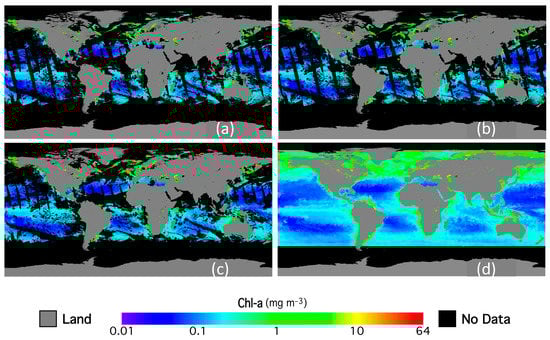
Figure 1.
The Visible Infrared Imaging Radiometer Suite (VIIRS)-measured global Level-3 Chl-a image on 21 June 2018 from (a) Suomi National Polar-Orbiting Partnership (SNPP), (b) National Oceanic and Atmospheric Administration (NOAA)-20, (c) merged VIIRS SNPP/NOAA-20 Chl-a image on the same day, and (d) gap-filled VIIRS SNPP/NOAA-20 merged Chl-a image on the same day.
2.2. Merging VIIRS SNPP and NOAA-20 Global Level-3 Ocean Color Data
As noted previously, SNPP and NOAA-20 operate at the same sun-synchronous polar orbit of 824-km. However, the positions of the two satellites in the orbit are intentionally arranged so that NOAA-20 leads SNPP by a half orbit, or ~50 minutes. The 50-minute difference between their paths makes the NOAA-20’s nadir points always running through SNPP’s gaps due to high sensor-zenith angle, and vice versa. This special arrangement of satellite positions in the orbit significantly benefits the observation of the ocean color from the space: the overlap of the spatial coverages of the two sensors fills most of each other’s gaps in images due to high sensor-zenith angles and high sun glint contamination, and significantly reduces the missing pixels in the merged images. In addition, ocean biological features are assumed to have little change in ~50 minutes, so that the ocean color data from the two sensors can be directly merged.
The VIIRS SNPP and NOAA-20 instruments both have 14 reflective solar bands (RSBs) with three image bands (I1–I3) and 11 moderate bands (M1–M11) operating in the spectral region of 0.41–2.25 µm. There are slight differences between VIIRS-SNPP and VIIRS-NOAA-20 in the nominal center wavelengths of each band. Table 1 lists the VIIRS RSB spectral band nominal center wavelength for VIIRS-SNPP and VIIRS-NOAA-20. In the ocean color data processing, the VIIRS-NOAA-20 nLw(λ) of five bands (M1–M5) are adjusted to match up with those of VIIRS-SNPP, so that Chl-a, Kd(490), and Kd(PAR) products are equivalent from the two sensors, and can be merged. In this study, only Chl-a products are merged as a preliminary test.
The VIIRS SNPP and NOAA-20 have the same swath width of 3040 km, and horizontal resolution of 750 m for M bands, and 375 m for I bands at nadir. With the same spatial and temporal resolutions, and their ocean color products processed using the same MSL12 software package, Chl-a data from the two instruments are statistically equivalent. Figure 2 shows the scatter plots of VIIRS NOAA-20 versus SNPP Chl-a data on 21 June 2018. The mean ratios of VIIRS NOAA-20/SNPP are 1.069, 1.024, 1.057, and 1.127 in global ocean, global oligotrophic waters (Chl-a < 0.1 mg/m3), global deep waters (water depth > 1 km), and global coastal and inland waters (water depth ≤ 1 km), respectively; and the corresponding standard deviation (SD) values are 0.212, 0.162, 0.175, and 0.336, respectively. Therefore, the statistics of the ocean color products from the two sensors are very close to each other, and they can be directly merged. In this study, the merged VIIRS SNPP/NOAA-20 ocean color products are calculated as weighted averages, where the weight is the number of valid pixels in each bin. The input datasets of the merging process are 30 days of daily SNPP and NOAA-20 global 9-km resolution Level-3 binned Chl-a data from June 19 to July 18, 2018, and the output data are merged SNPP/NOAA-20 global 9-km resolution data in Level-3 binned format.
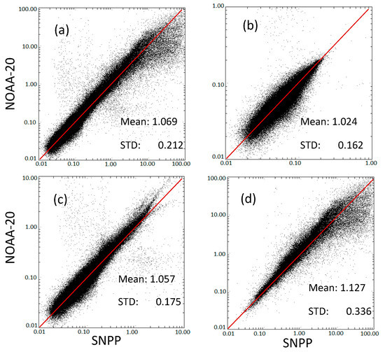
Figure 2.
Scatter plots of VIIRS NOAA-20 versus SNPP Chl-a in (a) global all regions, (b) global oligotrophic waters, (c) global deep waters, and (d) global coastal and inland waters on 21 June 2018.
2.3. Gap-Filling of the Merged VIIRS SNPP/NOAA-20 Data
The DINEOF method [23,24] is an Empirical Orthogonal Function (EOF)-based technique, which allows the extraction of the dominant spatial patterns observed in a data time series through an iterative approach, while simultaneously filling in the missing data. During the DINEOF process, the original dataset is first stored in a spatio-temporal matrix with m × n dimensions, where m is the number of grids in the spatial domain and n is the number of time steps in the time series. Initially, the temporal and spatial mean is removed from the data, and all missing values are set to zeroes. The first EOF mode is then calculated by using the singular value decomposition (SVD) technique, and the missing values are replaced with the initial guess by the data reconstruction using the spatial and temporal functions of only the first EOF mode. The first EOF mode is then recalculated iteratively using the previous best guess as the initial value of the missing data for the subsequent iteration until the process converges. Subsequently, the number of EOFs increases one by one and for each EOF mode, the whole reconstruction is operated again until convergence. Then, by using a cross-validation technique, the optimal number of EOF modes can be determined. Finally, the reconstruction procedure is performed again, based on the optimal EOF modes, until convergence is reached. The process to determine the optimum number of EOF modes in the final reconstruction is fully automatic. For example, if the error (reconstructed − original) of the validation pixels decreases gradually from mode 1 to mode 10, but the error starts to increase gradually from mode 11 to mode 13, then the first 10 modes are considered as optimum.
In this study, the DINEOF is utilized to reconstruct (gap-filled) the missing pixels in the merged VIIRS SNPP/NOAA-20 Chl-a data. Specifically, DINEOF is applied to 30 days of daily merged global Level-3 Chl-a data of 9-km spatial resolution from 19 June to 18 July 2018. It is noted that DINEOF is applied directly to the VIIRS Level-3 bin data files, rather than the mapped data files. However, it is a very large dataset for 30 days of global Chl-a data with 9-km spatial resolution, which makes the performance of DINEOF analysis very inefficient. To speed up the DINEOF process, the same procedure used for gap-filling of SNPP ocean color data by Liu and Wang [36] is used. Basically, the global dataset is evenly divided into 16 10°-zonal sections between 80°S and 80°N, and DINEOF is applied to each of the zonal sections separately. In fact, DINEOF analyses on the 16 zonal sections are performed in parallel to further improve data processing efficiency.
3. Results
3.1. Merged VIIRS SNPP/NOAA-20 Products
The VIIRS SNPP and NOAA-20 global daily Level-3 Chl-a data of 9-km spatial resolution, from 19 June to 18 July 2018, were merged. As an example, Figure 1c shows the merged SNPP/NOAA-20 Chl-a concentration on 21 June 2018. The spatial coverage of the merged ocean color data was significantly improved compared with either SNPP (Figure 1a) or NOAA-20 (Figure 1b). Particularly, in Figure 1a,b, the gaps of high sensor-zenith angle occurred in both the northern and southern hemisphere. The gaps of sun glint, however, occurred only to the north of the equator because it was summer (June–July) in the northern hemisphere. In Figure 1c, gaps of missing pixels due to the high sensor-zenith angle and high sun glint contamination from both VIIRS sensors were almost filled, thanks to the overlap of the swath of the two sensors. The remaining missing pixels were due to a very small part of high sensor-zenith angles from the one sensor and a small part of high sun glint contamination from the other. They were significantly reduced. It can be clearly seen in Figure 1c that the gaps of the missing pixels due to the high sensor-zenith angles and high sun glint contamination were much narrower than those in Figure 1a,b. In the southern hemisphere, however, it was completely free of gaps from sun glint contamination and high sensor-zenith angle. In addition, the missing pixels due to cloud cover were also reduced in the merged Chl-a image, because of the shifts of the cloud pixels during the 50-minute period. Overall, the merged VIIRS SNPP/NOAA-20 global Level-3 daily data had ~38% more valid pixels than those from the SNPP or NOAA-20 data alone.
The major gaps of missing pixels in the merged VIIRS SNPP/NOAA-20 data were due to cloud covers. Since there was only a 50-minute delay between the paths of the two satellites, cloud usually had little change in its shape, but could travel a short distance. The merging only reduced some limited pixels on the edges of the cloud cover, but the general pattern of gaps due to cloud cover was still the same in the merged data as in the SNPP or NOAA-20 data. Indeed, the merging could not improve spatial coverage in regions with large areas of thick clouds, such as in the Arabian Sea and Bay of Bengal, equatorial Atlantic Ocean, and high-latitude Pacific and Atlantic Oceans. The summer monsoon usually brings large amounts of moisture and rainfall to the Arabian Sea from June to July.
3.2. Gap-Filled VIIRS SNPP/NOAA-20 Products
The DINEOF method was applied to the merged VIIRS SNPP/NOAA-20 global daily Level-3 Chl-a data from 19 June to 18 July 2018. The DINEOF has two options to reconstruct missing data: fully reconstructed images and filled images. A fully reconstructed image was calculated from the retained EOF modes using the DINEOF method. In the fully reconstructed image, all ocean color data were reconstructed on every ocean pixel (including non-missing pixels). The reconstructed image had no-gaps spatially. However, there were some small differences between reconstructed and original data even for non-missing pixels due to truncated EOF modes in computing all data values. The filled image was a combination of the original image and the reconstructed image, i.e., missing pixels were filled with reconstructed data and original data were kept for non-missing pixels. As an example, the fully reconstructed global Chl-a image of 21 June 2018 is shown in Figure 1d. All gaps of missing pixels due to the high sun glint and large sensor-zenith angles were filled with valid pixels. The gaps of cloud-covered pixels were also reconstructed, especially in the northern Atlantic and Pacific, Arabian Sea and Bay of Bengal, and the equatorial Atlantic Ocean as well. The gaps of missing pixels were all filled very smoothly in Figure 1d. However, the large area of missing pixels in the Southern Ocean close to Antarctica were not reconstructed, since there were no valid pixels in the entire area from 19 June to 18 July 2018 due to high solar-zenith angles during the northern hemisphere summer time.
To evaluate the accuracy of the value from reconstructed pixels, 5% of valid (non-missing) pixels in the original Level-3 data were randomly selected, and intentionally treated as “missing pixels.” These pixels were reconstructed and compared with the original data for validation. Figure 3 shows the density scatter plots of the reconstructed data versus original data in the global ocean, oligotrophic waters, deep waters, and coastal and inland waters. In general, most points are close to the 1:1 line in the global ocean, but the oligotrophic waters show the best results (Figure 3b), whilst the highest level of scatter is found in the coastal and inland waters (Figure 3d). Quantitatively, the mean and SD of the reconstructed/original ratios in oligotrophic water are 1.012 and 0.164, respectively. The mean and SD in deep waters are 1.015 and 0.182, respectively, which are slightly higher than those in oligotrophic waters. In the coastal and inland waters, the mean and SD are 0.997 and 0.287, respectively. Overall, for all pixels in the global ocean, the mean and SD of the reconstructed/original ratios are 1.012 and 0.200, respectively. It is noted that the locations of the validation pixels are selected randomly using the random number generator in the Interactive Data Language (IDL). In addition, the DINEOF package includes a built-in function to specify the “size of cloud surface” for cross-validation as a parameter of input. We tested the cross-validation with different cloud patch sizes and found that the cross-validation result does not change significantly with the size of the cloud surface. The main reason is that DINEOF considers not only spatial coherence, but also temporal coherence. Since the location of the cloud patches are selected randomly, even with the large size of cloud patch, the temporal variations in the time-series can still be used to infer the missing values. The advantage of the DINEOF over traditional interpolation is that it utilizes major EOF modes to reconstructs the missing pixels, which capture the major signals of variations in both spatial and temporal domains simultaneously.
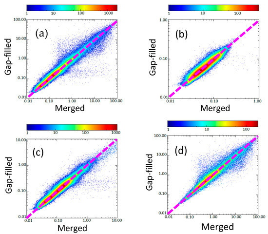
Figure 3.
Density scatter plots of gap-filled versus merged Chl-a values for (a) all selected validation pixels, (b) oligotrophic waters, (c) deep waters, and (d) coastal and inland waters on 21 June 21 2018.
3.3. Ocean Features Revealed in the Gap-Filled VIIRS SNPP/NOAA-20 Chl-a Data
Gap-filled daily Chl-a images reveal many large-scale and meso-scale ocean features that are invisible in the merged Chl-a images, or the original VIIRS SNPP, NOAA-20 Chl-a images. As shown in Figure 1d, the most obvious large-scale ocean features are the oligotrophic waters (Chl-a < 0.1 mg/m3) in the center of the five subtropical ocean gyres, i.e., North Atlantic, South Atlantic, North Pacific, South Pacific, and South Indian Ocean, which cover major parts of the global oceans. Because of the easterly winds near the equator and the equatorial upwelling, there is more enhanced Chl-a concentration (~0.1–0.5 mg/m3) in the equatorial Pacific Ocean and equatorial Atlantic Ocean regions than in the subtropical gyres. However, no significant Chl-a enhancement is found in the equatorial Indian Ocean. In addition, the Gulf Stream in the North Atlantic Ocean and Kuroshio in the North Pacific Ocean mark a clear boundary in the high latitude ocean regions: high Chl-a concentrations are found to the north of the boundary, while low Chl-a to the south.
In addition to these large-scale features, the gap-filled images also reveal many meso-scale ocean features, such as eddies and filaments associated with western boundary currents or coastal currents. Figure 4 shows the transformation of meso-scale eddies in the Gulf of Mexico (GOM) from 19 June to 18 July 2018. Ocean circulation in the GOM is dominated by the loop current (LC), an extension of the western boundary current system of the North Atlantic Ocean that loops into the GOM. The LC enters the Gulf through the Yucatan Channel and exits through the Florida Straits. The LC occasionally extends further northward into the GOM, approaching the northern shelf break. This long extension of the loop will eventually separate to form an anticyclonic loop current eddy (LCE). Formation of an LCE by separation from the LC happens irregularly every several months, and there can be a number of LCEs in the GOM at one time. Figure 4 shows three LCEs in the GOM: two of them (A and B) were aged LCEs that already moved to the west side of GOM, and one (C) was a new LCE that just separated from the LC. Loop current eddy A and B are about 100 km in diameter, and C is about 200 km in diameter. During the one-month period from 19 June to 18 July 2018, A and B were still moving continuously to the west, and A was showing some changes in its shape while interacting with the LC. The LC was very flat till 7 July, when the LC started to bulge northward, getting ready to shed a new LCE. The details of the transformation of these meso-scale ocean features were not available in either SNPP, NOAA-20, or in the merged images, but only revealed in the gap-filled images. The transitions of these meso-scale ocean features were very smooth both temporally and spatially. To compare with the original VIIRS images without gap-fillings, Chl-a global daily images from SNPP, NOAA-20, or merged SNPP/NOAA-20 can be found in the NOAA Ocean Color Team website (https://www.star.nesdis.noaa.gov/sod/mecb/color/), in particular, using the powerful image display tool, i.e., the Ocean Color Viewer (OCView) [48]. With OCView, the user can zoom in to the GOM region (or any other region) with high spatial resolution (2 km) images, and select SNPP, NOAA-20 or the merged SNPP/NOAA-20 images.
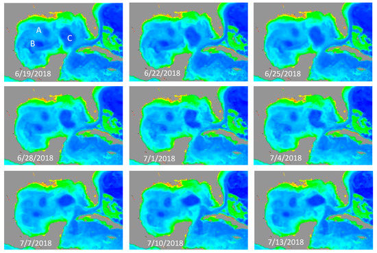
Figure 4.
Daily Chl-a images of the Gulf of Mexico (GOM) from 19 June to 13 July 2018 with three loop current eddies (A, B, and C) marked on the 19 June 2018 Chl-a image.
3.4. Comparison with Gap-Filled Data Based on VIIRS SNPP or NOAA-20
The DINEOF was also applied to Chl-a data from a single sensor, VIIRS-SNPP or VIIRS-NOAA-20, and the gap-filled data based on a single sensor were compared with gap-filled data based on the merged products. Figure 5 shows the gap-filled data based on VIIRS-SNPP, VIIRS-NOAA-20, and merged VIIRS SNPP/NOAA-20 products in the GOM on 21 June, 30 June, and 18 July 2018, as examples. It can be seen that, in general, the gap-filled data based on the merged products show the same pattern as those based on SNPP or NOAA-20 alone. However, there are more details in the dynamic features in the gap-filled data based on the merged product than those based on SNPP or NOAA-20 alone, and the interactions of the loop current with surrounding eddies are different in the merged products. On 21 June, the gap-filled data based on merged VIIRS SNPP/NOAA-20 products (Figure 5c) show more details in the coastal eddy feature “A” than VIIRS-SNPP (Figure 5a) or VIIRS-NOAA-20 (Figure 5b) alone. On 30 June 2018, the feature of the big eddy “B” are different in the gap-filled data based on merged products (Figure 5f). From 30 June to 18 July, the eddy “B” was pushed northward by the loop current, and transformed from a north–south oriented shape to a west–east oriented shape. In the animation of the daily images (not shown here), the interactions of the eddy “B” with the loop current were more clearly shown in the merged products. On 18 July 2018, the eddy “C” was seen more clearly in Figure 5i than that in Figure 5g or Figure 5h. Generally, the merged data have more spatial coverage than that from either SNPP or NOAA-20 alone. Indeed, some ocean dynamic features could be partially blocked by pixels with high sensor-zenith angle, sun glint, or cloud in VIIRS SNPP or NOAA-20 images. But, merging data from the two sensors can significantly increase valid pixels in the coverage. Consequently, the gap-filled ocean color products based on the merged data set can capture more details of the ocean dynamic features.
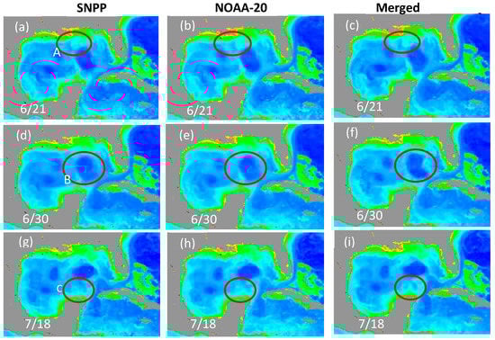
Figure 5.
Comparison of the VIIRS-derived ocean features in the GOM in the gap-filled images based on SNPP (left column), NOAA-20 (middle column), and SNPP/NOAA-20 merged (right column) data in 2018 on 21 June (top row) (a–c), 30 June (middle row) (d–f), and 18 July (bottom row) (g–i).
4. Discussion and Conclusions
In a recent study [36], we used the DINEOF to fill the gaps of missing pixels in daily VIIRS-SNPP ocean color data, and it was demonstrated that the DINEOF method can successfully reconstruct and reveal meso-scale and large-scale spatial ocean features in the global VIIRS Level-3 images, as well as capture the temporal variations of these features. Based on the same methodology, in this study, the DINEOF was applied on the daily merged VIIRS SNPP/NOAA-20 global Level-3 ocean Chl-a data. The VIIRS-SNPP and VIIRS-NOAA-20 have very similar sensor characteristics, and the statistics of the ocean color data derived from the two sensors are very close to each other. In addition, global VIIRS SNPP and NOAA-20 ocean color data are derived using the same MSL12 ocean color data processing system. As shown in examples, merging VIIRS-SNPP and VIIRS-NOAA-20 data almost removes the gaps of missing pixels due to high sensor-zenith angles and high sun glint contamination, and also significantly reduces the gaps due to cloud cover. The remaining regular gaps in the merged images are due to small gaps from high sensor-zenith angles in one sensor and sun glint contamination in another. Overall, there are ~38% more valid ocean color pixels in the merged VIIRS SNPP/NOAA 20 global Level-3 daily data than those in the SNPP or NOAA-20 data alone.
In the gap-filled Chl-a data, all missing pixels due to the high sensor-zenith angle and high sun glint were mostly reconstructed. The gaps of cloud-covered pixels were also reconstructed, especially in regions with large areas of thick clouds, such as in the northern Atlantic and Pacific, Arabian Sea and Bay of Bengal, and the equatorial Atlantic Ocean as well. Quantitatively, the mean ratios of the reconstructed/original data are 1.012, 1.012, 1.015, and 0.997 for the global ocean, global oligotrophic waters, global deep waters, and global coastal and inland waters, respectively; and the corresponding SD values are 0.200, 0.164, 0.182, and 0.287, respectively. Gap-filled daily Chl-a images reveal many large-scale and meso-scale ocean features and their variations, which are invisible in the original VIIRS-SNPP or VIIRS-NOAA-20 Chl-a images.
The gap-filled Chl-a data based on two-sensor merged products were compared with gap-filled data based on single sensor VIIRS-SNPP or VIIRS-NOAA-20 alone. It is demonstrated that the gap-filled data based on the merged products show more details in the ocean features than those based on a single sensor alone, and there are differences in the dynamics of ocean features. This is an important message that adding more sensors into the merged products will significantly improve the quality of gap-filled ocean color data. Previous missions such as the Sea-viewing Wide Field-of-view Sensor (SeaWiFS) (1997–2010), MODIS on the Terra (1999–present) and Aqua (2002–present) satellites, and the Medium-Resolution Imaging Spectrometer (MERIS) on the ENVISAT (2002–2012) had provided long-term high-quality global ocean color data to the community. Currently, in addition to the VIIRS on SNPP and NOAA-20, the Ocean and Land Color Instrument (OLCI) on the Sentinel-3A (2016–present) and Sentinel-3B (2018–present) satellites, and the Second-Generation Global Imager (SGLI) on the Global Change Observation Mission-Climate (GCOM-C) (2017–present) are all providing an unprecedented view of ocean optical, biological, and biogeochemical properties on a global scale simultaneously. Adding these sensors in the data merging process will significantly improve the spatial coverage in the merged global ocean color data, and the quality of gap-filled ocean color data as well.
Author Contributions
X.L. carried out the main research work for developing algorithm, obtaining the results, and analyzing the data. M.W. suggested the topic and contributed to the algorithm development and evaluation.
Funding
This work was supported by the Joint Polar Satellite System (JPSS) funding and NOAA Product Development, Readiness, and Application (PDRA)/Ocean Remote Sensing (ORS) Program funding.
Acknowledgments
We thank two anonymous reviewers for their useful comments. The views, opinions, and findings contained in this paper are those of the authors and should not be construed as an official NOAA or U.S. Government position, policy, or decision.
Conflicts of Interest
The authors declare no conflict of interest.
References
- Yoder, J.A.; Doney, S.C.; Siegel, D.A.; Wilson, C. Study of marine ecosystem and biogeochemistry now and in the future: Example of the unique contributions from the space. Oceanography 2010, 23, 104–117. [Google Scholar] [CrossRef]
- Goldberg, M.D.; Kilcoyne, H.; Cikanek, H.; Mehta, A. Joint Polar Satellite System: The United States next generation civilian polar-orbiting environmental satellite system. J. Geophys. Res. Atmos. 2013, 118, 13463–13475. [Google Scholar] [CrossRef]
- Wang, M.; Liu, X.; Tan, L.; Jiang, L.; Son, S.; Shi, W.; Rausch, K.; Voss, K. Impact of VIIRS SDR performance on ocean color products. J. Geophys. Res. Atmos. 2013, 118, 10347–10360. [Google Scholar] [CrossRef]
- Wang, M.; Shi, W.; Jiang, L.; Voss, K. NIR- and SWIR-based on-orbit vicarious calibrations for satellite ocean color sensors. Opt. Express 2016, 24, 20437–20453. [Google Scholar] [CrossRef] [PubMed]
- O’Reilly, J.E.; Maritorena, S.; Mitchell, B.G.; Siegel, D.A.; Carder, K.L.; Garver, S.A.; Kahru, M.; McClain, C.R. Ocean color chlorophyll algorithms for SeaWiFS. J. Geophys. Res. 1998, 103, 24937–24953. [Google Scholar] [CrossRef]
- Hu, C.; Lee, Z.; Franz, B.A. Chlorophyll a algorithms for oligotrophic oceans: A novel approach based on three-band reflectance difference. J. Geophys. Res. 2012, 117, C01011. [Google Scholar] [CrossRef]
- Wang, M.; Son, S. VIIRS-derived chlorophyll-a using the ocean color index method. Remote Sens. Environ. 2016, 182, 141–149. [Google Scholar] [CrossRef]
- Gordon, H.R.; Wang, M. Retrieval of water-leaving radiance and aerosol optical thickness over the oceans with SeaWiFS: A preliminary algorithm. Appl. Opt. 1994, 33, 443–452. [Google Scholar] [CrossRef]
- Wang, M. (Ed.) Atmospheric Correction for Remotely-Sensed Ocean-Colour Products; Reports of International Ocean-Colour Coordinating Group IOCCG: Dartmouth, NS, Canada, 2010. [Google Scholar] [CrossRef]
- Wang, M.; Jiang, L. VIIRS-derived ocean color product using the imaging bands. Remote Sens. Environ. 2018, 206, 275–286. [Google Scholar] [CrossRef]
- Wang, M.; Son, S.; Harding, J.L.W. Retrieval of diffuse attenuation coefficient in the Chesapeake Bay and turbid ocean regions for satellite ocean color applications. J. Geophys. Res. 2009, 114, C10011. [Google Scholar] [CrossRef]
- Son, S.; Wang, M. Diffuse attenuation coefficient of the photosynthetically available radiation Kd(PAR) for global open ocean and coastal waters. Remote Sens. Environ. 2015, 159, 250–258. [Google Scholar] [CrossRef]
- Lee, Z.P.; Carder, K.L.; Arnone, R.A. Deriving inherent optical properties from water color: A multiple quasi-analytical algorithm for optically deep waters. Appl. Opt. 2002, 41, 5755–5772. [Google Scholar] [CrossRef] [PubMed]
- Shi, W.; Wang, M. Characterization of particle backscattering of global highly turbid waters from VIIRS ocean color observations. J. Geophys. Res. Oceans 2017, 122, 9255–9275. [Google Scholar] [CrossRef]
- Wei, J.; Lee, Z.; Shang, S. A system to measure the data quality of spectral remote-sensing reflectance of aquatic environments. J. Geophys. Res. Oceans 2016, 121, 8189–8207. [Google Scholar] [CrossRef]
- Wang, M.; Shi, W. Estimation of ocean contribution at the MODIS near-infrared wavelengths along the east coast of the U.S.: Two case studies. Geophys. Res. Lett. 2005, 32, L13606. [Google Scholar] [CrossRef]
- Wang, M.; Shi, W.; Tang, J. Water property monitoring and assessment for China’s inland Lake Taihu from MODIS-Aqua measurements. Remote Sens. Environ. 2011, 115, 841–854. [Google Scholar] [CrossRef]
- Wang, M.; Son, S.; Shi, W. Evaluation of MODIS SWIR and NIR-SWIR atmospheric correction algorithm using SeaBASS data. Remote Sens. Environ. 2009, 113, 635–644. [Google Scholar] [CrossRef]
- Wang, M. Remote sensing of the ocean contributions from ultraviolet to near-infrared using the shortwave infrared bands: Simulations. Appl. Opt. 2007, 46, 1535–1547. [Google Scholar] [CrossRef]
- Wang, M.; Shi, W. The NIR-SWIR combined atmospheric correction approach for MODIS ocean color data processing. Opt. Express 2007, 15, 15722–15733. [Google Scholar] [CrossRef]
- Sun, J.; Wang, M. Radiometric calibration of the VIIRS reflective solar bands with robust characterizations and hybrid calibration coefficients. Appl. Opt. 2015, 54, 9331–9342. [Google Scholar] [CrossRef]
- Sun, J.; Chu, M.; Wang, M. On-orbit characterization of the VIIRS solar diffuser and attenuation screens for NOAA-20 using yaw measurements. Appl. Opt. 2018, 57, 6605–6619. [Google Scholar] [CrossRef] [PubMed]
- Alvera-Azcarate, A.; Barth, A.; Rixen, M.; Beckers, J. Reconstruction of incomplete oceanographic data sets using Empirical Orthogonal Functions. Application to the Adriatic Sea. Ocean Model. 2005, 9, 325–346. [Google Scholar] [CrossRef]
- Beckers, J.; Rixen, M. EOF calculations and data filling from incomplete oceanographic data sets. J. Atmos. Ocean Technol. 2003, 20, 1839–1856. [Google Scholar] [CrossRef]
- Ganzedo, U.; Alvera-Azcarate, A.; Esnaola, G.; Ezcurra, A.; Saenz, J. Reconstruction of sea surface temperature by means of DINEOF. A case study during the fishing season in the Bay of Biscay. Int. J. Remote Sens. 2011, 32, 933–950. [Google Scholar] [CrossRef]
- Mauri, E.; Poulain, P.M.; Juznic-Zontac, Z. MODIS chlorophyll variability in the northern Adriatic Sea and relationship with forcing parameters. J. Geophys. Res. 2007, 112, C03S11. [Google Scholar] [CrossRef]
- Mauri, E.; Poulain, P.M.; Notarstefano, G. Spatial and temporal variability of the sea surface temperature in the Gulf of Trieste between January 2000 and December 2006. J. Geophys. Res. 2008, 113, C10012. [Google Scholar] [CrossRef]
- Nechad, B.; Alvera-Azcarate, A.; Ruddick, K.; Greenwood, N. Reconstruction of MODIS total suspended matter time series maps by DINEOF and validation with autonomous platform data. Ocean Dyn. 2011, 61, 1205–1214. [Google Scholar] [CrossRef]
- Sirjacobs, D.; Alvera-Azcarate, A.; Barth, A.; Lacroix, G.; Park, Y.; Nechad, B.; Ruddick, K.; Beckers, J. Cloud filling of ocean color and sea surface temperature remote sensing products over the Southern North Sea by the data interpolating empirical orthogonal functions methodology. J. Sea Res. 2011, 65, 114–130. [Google Scholar] [CrossRef]
- Volpe, G.; Nardelli, B.B.; Cipollini, P.; Santoleri, R.; Robinson, I.S. Seasonal to interannual phytoplankton response to physical processes in the Mediterranean Sea from satellite observations. Remote Sens. Environ. 2012, 117, 223–235. [Google Scholar] [CrossRef]
- Li, Y.; He, R. Spatial and temporal variability of SST and ocean color in the Gulf of Maine based on cloud-free SST and chlorophyll reconstructions in 2003–2012. Remote Sens. Environ. 2014, 144, 98–108. [Google Scholar] [CrossRef]
- Moradi, M.; Kabiri, K. Spatio-temporal variability of SST and chlorophyll-a from MODIS data in the Persian Gulf. Mar. Pollut. Bull. 2015, 98, 14–25. [Google Scholar] [CrossRef] [PubMed]
- Hilborn, A.; Costa, M. Applications of DINEOF to Satellite-Derived Chlorophyll-a from a Productive Coastal Region. Remote Sens. 2018, 10, 1449. [Google Scholar] [CrossRef]
- Alvera-Azcarate, A.; Vanhellemont, Q.; Ruddick, K.G.; Barth, A.; Beckers, J.-M. Analysis of high frequency geostationary ocean colour data using DINEOF. Estuarine Coast. Shelf Sci. 2015, 159, 28–36. [Google Scholar] [CrossRef]
- Liu, X.; Wang, M. Analysis of diurnal variations from the Korean Geostationary Ocean Color Imager measurements using the DINEOF method. Estuarine Coast. Shelf Sci. 2016, 180, 230–241. [Google Scholar] [CrossRef]
- Liu, X.; Wang, M. Gap filling of missing data for VIIRS global ocean color product using the DINEOF method. IEEE Trans. Geosci. Remote Sens. 2018, 56, 4464–4476. [Google Scholar] [CrossRef]
- Wang, M. A sensitivity study of SeaWiFS atmospheric correction algorithm: Effects of spectral band variations. Remote Sens. Environ. 1999, 67, 348–359. [Google Scholar] [CrossRef]
- Wang, M.; Franz, B.A. Comparing the ocean color measurements between MOS and SeaWiFS: A vicarious intercalibration approach for MOS. IEEE Trans. Geosci. Remote Sens. 2000, 38, 184–197. [Google Scholar] [CrossRef]
- Wang, M.; Isaacman, A.; Franz, B.A.; McClain, C.R. Ocean color optical property data derived from the Japanese Ocean Color and Temperature Scanner and the French Polarization and Directionality of the Earth’s Reflectances: A comparison study. Appl. Opt. 2002, 41, 974–990. [Google Scholar] [CrossRef]
- Wang, M.; Jiang, L. Atmospheric correction using the information from the short blue band. IEEE Trans. Geosci. Remote Sens. 2018, 56, 6224–6237. [Google Scholar] [CrossRef]
- Shi, W.; Wang, M. Satellite views of the Bohai Sea, Yellow Sea, and East China Sea. Prog. Oceanogr. 2012, 104, 35–45. [Google Scholar] [CrossRef]
- Shi, W.; Wang, M.; Jiang, L. Spring-neap tidal effects on satellite ocean color observations in the Bohai Sea, Yellow Sea, and East China Sea. J. Geophys. Res. 2011, 116, C12032. [Google Scholar] [CrossRef]
- Shi, W.; Wang, M. Ocean reflectance spectra at the red, near-infrared, and shortwave infrared from highly turbid waters: A study in the Bohai Sea, Yellow Sea, and East China Sea. Limnol. Oceanogr. 2014, 59, 427–444. [Google Scholar] [CrossRef]
- Campbell, J.W.; Blaisdell, J.M.; Darzi, M. Level-3 SeaWiFS Data Products: Spatial and Temporal Binning Algorithms. Oceanogr. Lit. Rev. 1996, 9, 952. [Google Scholar]
- Wang, M.; Shi, W. Cloud masking for ocean color data processing in the coastal regions. IEEE Trans. Geosci. Rem. Sens. 2006, 44, 3196–3205. [Google Scholar] [CrossRef]
- Jiang, L.; Wang, M. Identification of pixels with stray light and cloud shadow contaminations in the satellite ocean color data processing. Appl. Opt. 2013, 52, 6757–6770. [Google Scholar] [CrossRef] [PubMed]
- Wang, M.; Bailey, S.W. Correction of the sun glint contamination on the SeaWiFS ocean and atmosphere products. Appl. Opt. 2001, 40, 4790–4798. [Google Scholar] [CrossRef] [PubMed]
- Mikelsons, M.; Wang, M. Interactive online maps make satellite ocean data accessible. EOS 2018, 99. [Google Scholar] [CrossRef]
© 2019 by the authors. Licensee MDPI, Basel, Switzerland. This article is an open access article distributed under the terms and conditions of the Creative Commons Attribution (CC BY) license (http://creativecommons.org/licenses/by/4.0/).