Article

Thermo-Physical and Geo-Mechanical Characterization of Faulted Carbonate Rock Masses (Valdieri, Italy)

Dipartimento di Scienze della Terra, Università di Torino, 10125 Turin, Italy
*
Author to whom correspondence should be addressed.
Remote Sens. 2019, 11(2), 179; https://doi.org/10.3390/rs11020179
Submission received: 1 December 2018 / Revised: 10 January 2019 / Accepted: 13 January 2019 / Published: 18 January 2019
(This article belongs to the Special Issue Remote Sensing of Engineering Geological Science)

Abstract

:
Water in rock masses is a key factor in geo-mechanics, hydrogeology, mining, geo-thermics, and more. It is relevant in interpreting rock mass behavior (e.g., water-rock interaction or slope stability), as well as in defining heat transfer mechanisms. Pointing out the contribution of secondary porosity in increasing advective heat transfer instead of the conduction phenomenon, this study aims to highlight a different thermal response of sound rocks and faulted zones. Moreover, it provides some methodological suggestions to minimize environment disturbance in data collection and a robust interpretation of the results. An interesting outcrop was identified in a carbonate quarry near Valdieri (north-west Italian Alps): it was studied coupling a geo-mechanical and a thermo-physical approach. In particular, geo-mechanical and photogrammetric surveys, InfraRed Thermography (IRT), and Thermal Conductivity (TC) measurements were conducted. The rationale of the research is based on the fact that, when a substantial temperature difference between flowing groundwater and rocks was detected, IRT can reveal information about geo-mechanical and hydrogeological properties of the rock masses such as a degree of fracturing and joint interconnection. A comparative field and laboratory analysis using different devices enabled a more detailed insight providing values in both dry and wet conditions. A different thermal response was highlighted for the cataclastic zone as well. IRT results showed an evident inverse relationship among the number of joints per meter and the detected surface temperature. This is probably caused by the higher water flow within the cataclastic fault zone. Moreover, low fractured portions of the rock mass presented higher cooling rates and conducted heat far more than those with poor geo-mechanical characteristics (difference up to 40%). A negligible ratio between wet and dried thermal conductivity (about 1%) was also detected in lab measurements, which confirmed that primary porosity is not usually relevant in influencing thermal properties of the sound rock.

Graphical Abstract

1. Introduction

Groundwater flow in fractured rock masses has been studied by many earth scientists. It reveals one of the most important factors to be considered in slope stability problems [1,2,3] as well as in the hydrogeological assessment and in heat transfer mechanisms [4,5]. In particular, understanding geo-mechanical features, thermo-physical patterns, and their relationship with groundwater flow, is particularly important when facing non-homogeneous rock masses (flysches, calcschists, or faulted hard rock lithologies). The presence of groundwater flow can significantly improve the heat transfer mechanism [5], which increases the general heat budget. If the groundwater flow is negligible, the subsurface system is heat-conduction dominated and the amount of heat stored and removed depends only on the rate at which heat is conducted through the geologic media. When the groundwater flow is relevant, heat removal via conduction can be negligibly small because heat is rapidly dissipated through convection or advection [6]. A relevant advective heat transfer can be ruled by the presence of fractures acting as secondary porosity and making the rock mass even much more permeable than the matrix.
In order to understand groundwater paths, as well as its discharge and role, a complete characterization of rock masses is essential, especially regarding the definition of orientation, aperture, persistence, and interconnection of discontinuities [7]. This kind of information is usually obtained through geo-mechanical surveys. On the other hand, since water flow with a different temperature than surrounding medium can produce a thermal anomaly, a supplemental remote survey technique as the Infrared Thermography (IRT) coupled with Thermal Conductivity (TC) measures can provide useful data too.
IRT is widely applied in civil engineering and architecture especially for building diagnostics and insulation inspections [8,9]. In Earth Sciences, it is mainly used for the surveillance of volcanic systems [10], to calculate lava discharge rates [11] and fumarole emissions [12,13]. Reference [14] resume an interesting application, such as the study of heat capacity of rocky walls and monitoring of waste disposal sites. Moreover, some authors [15,16,17] used IRT to characterize the thermal response of rocks and joints, as well as landslide mapping [18,19,20,21]. On the other hand, TC measurement techniques are usually applied in engineering to test buildings materials, such as concrete and insulations [22], in the electronics industry [23], in developing new materials (e.g., nanomaterials and polymers, [24]), and for fire prevention [25]. Furthermore, thermal conductivity methods are widely employed in the Earth sciences such as testing heat transfer from rocks and soils [26] to evaluate thermal evolution of oil-bearing basins [27], to assess the thermal potential for geothermal exploration [28,29,30], or aim at the study of the Earth’s thermal regime [31,32]. This study aims to recognize different thermal behaviors between sound rocks and faulted zones.
In this context, an interesting test site located in a carbonate quarry in the Argentera Massif (Southern Piedmont, Italian Western Alps) was identified. In this case, a well exposed fault with a clear cataclastic belt is easy to reach and to photograph, so it is a very good site where both the cataclastic fault zone and the sound rock can be compared. In detail, the following was completed.
  • Geo-mechanical and a photogrammetric survey of the faults and the surroundings to characterize the rock mass;
  • time-lapse sequences of IRT thermal images in order to detect thermal transient within both the fault zone and the low fractured mass rock sectors;
  • thermal conductivity measurements to characterize thermal properties of rocks.
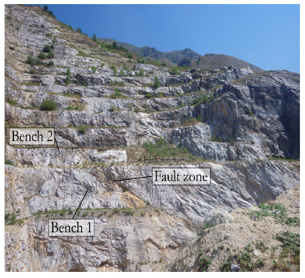
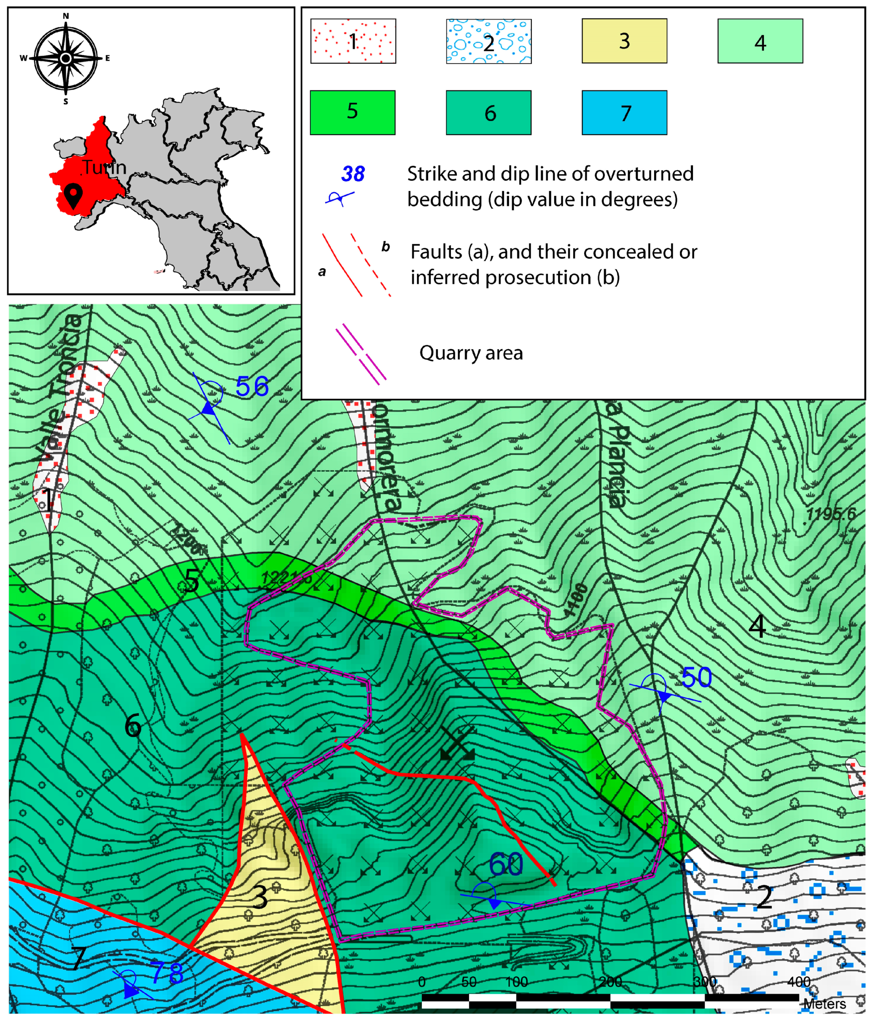
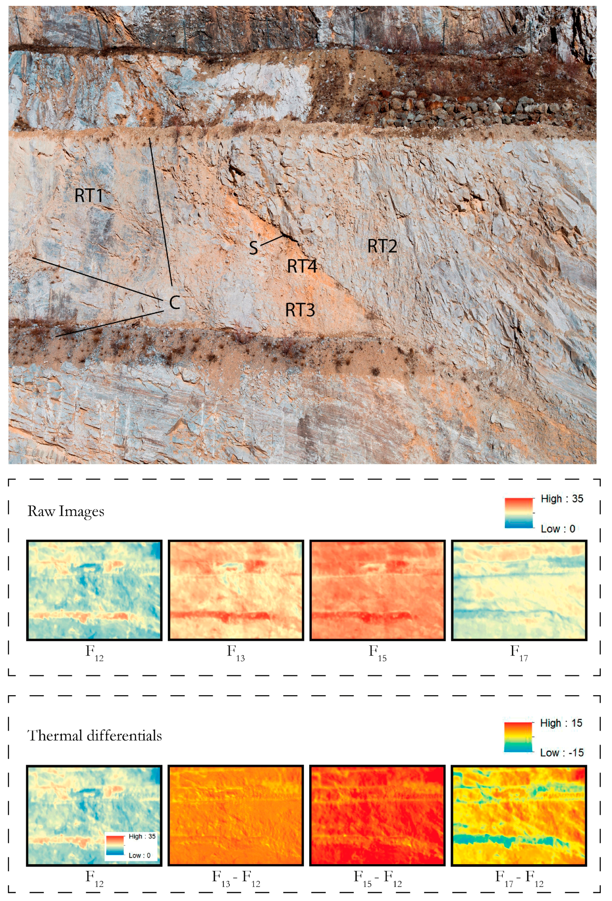
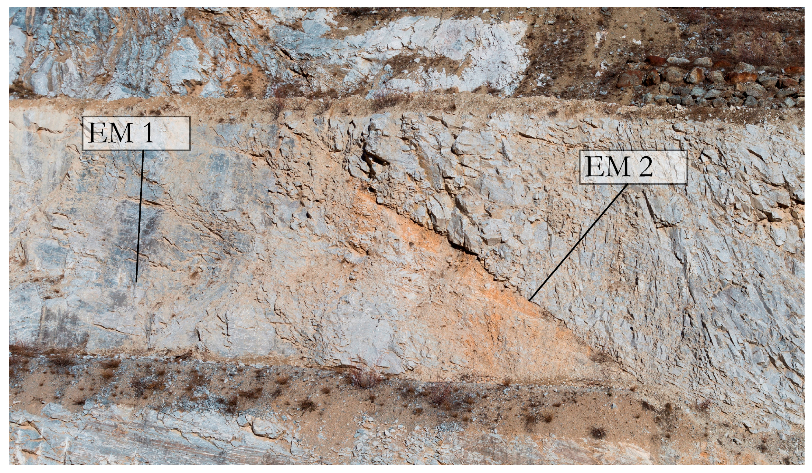
In detail, efforts were focused on comparing IRT and TC data with geo-mechanical parameters acquired on two scanlines following a standard ISRM procedure. In addition, a photogrammetric modelling of the area was conducted, and its derivative products such the orthomosaic and the texturized 3D model were used to double check the geo-mechanical features.

2. Study Site

The quarry is located close to the village of S. Lorenzo di Valdieri, nearby Cuneo village (North-Western Alps, Piedmont, Italy, Figure 1 and Figure 2). The geological units outcropping in the area belong to the Middle Jurassic–Lower Cretaceous Provençal succession located at the North-Eastern side of the Argentera Massif. The quarry produces pure calcium carbonate (99.9% volume of Calcite, Carbocalcio Cuneese S.p.A., and personal communication) treated and selected for sale as granulated and micronized.
The carbonate rock mass (Lausa Limestone) consists of fine-grained limestone, with abundant decimeter-thick beds of polymictic breccias, generally clast-supported, and with millimeter to decimeter sized clasts of mudstones, coarsely crystalline dolostones and finely crystalline dolostones. Lausa Limestones are followed by grey mudstones and crinoid-rich wackestones, in centimeter to decimeter thick beds, with abundant silicified portions. Fault rocks (Carnieules) and Entracque Marl outcrops toward SW while, in the uppermost part of the quarry, Aptian–upper Cretaceous rocks (Puriac Limestones and Marne Nere fm.) are present (Figure 2). Carbonates are locally affected by a diffuse hydrothermal dolomitization occurring in the Early Cretaceous period at a very shallow burial depth, which is related to the expulsion of hot fluids (about 200 °C) through faults and fractures during episodes of fault activity. The studied outcrop can be considered as belonging to the Valdieri Marbles according to Reference [33].
The quarry is at an elevation roughly between 900 and 1250 m. The front has an envelope slope of approximatively 53° and the dip direction is southeast (about 125°). It is structured in benches (10 m high, 2–2.5 m wide). The dip of the single terrace face is approximatively 62°–65° with local situations of greater acclivity. The front perpendicular to the cultivation has an envelope slope of approximatively 45° and is set on the schistosity planes. The dip direction of the front envelope is towards the South-West (about 200°). The dip of the single step elevation is that of the schistosity and is approximately equal to 50° but is locally higher.

3. Procedure and Methods

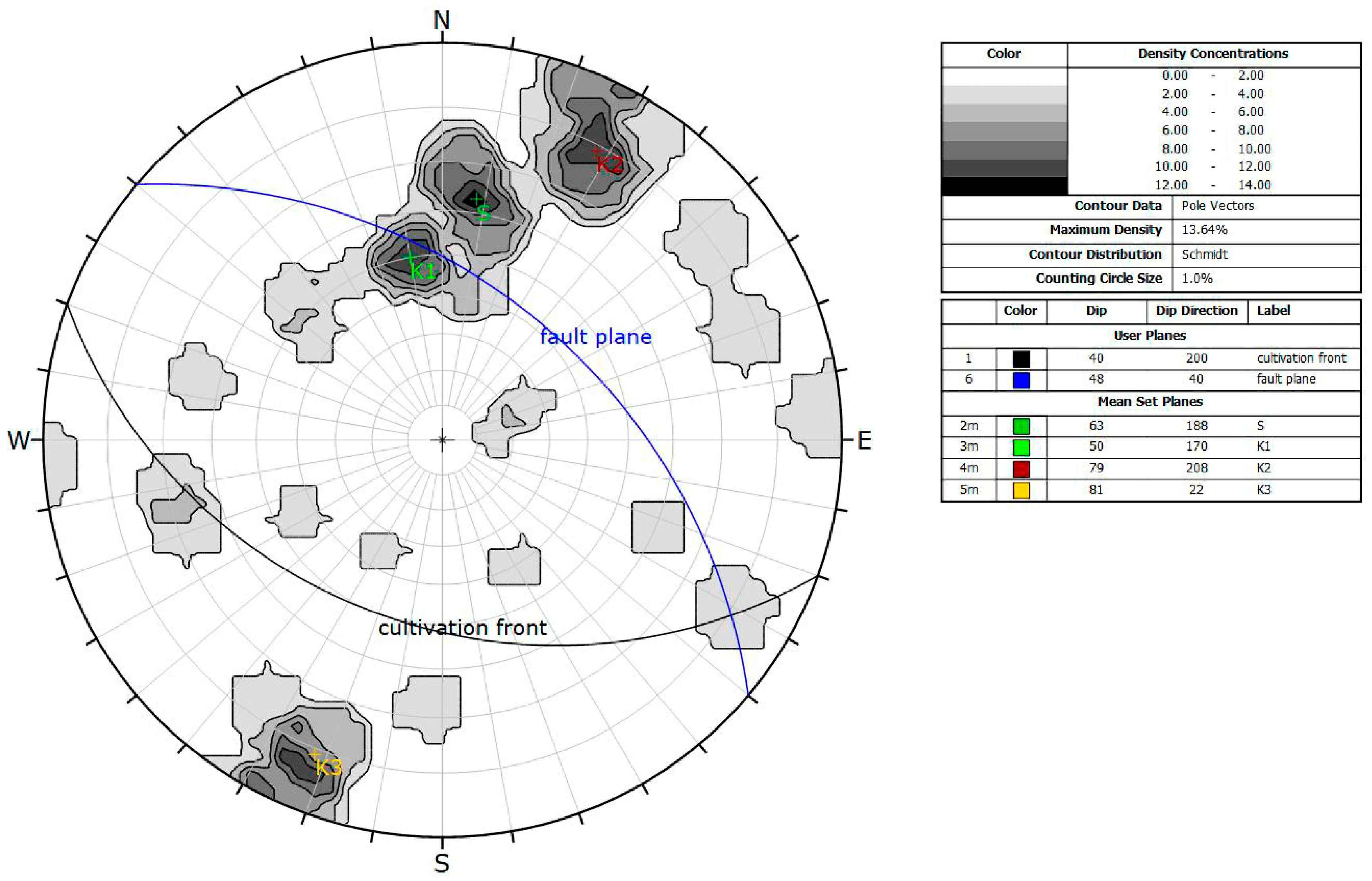
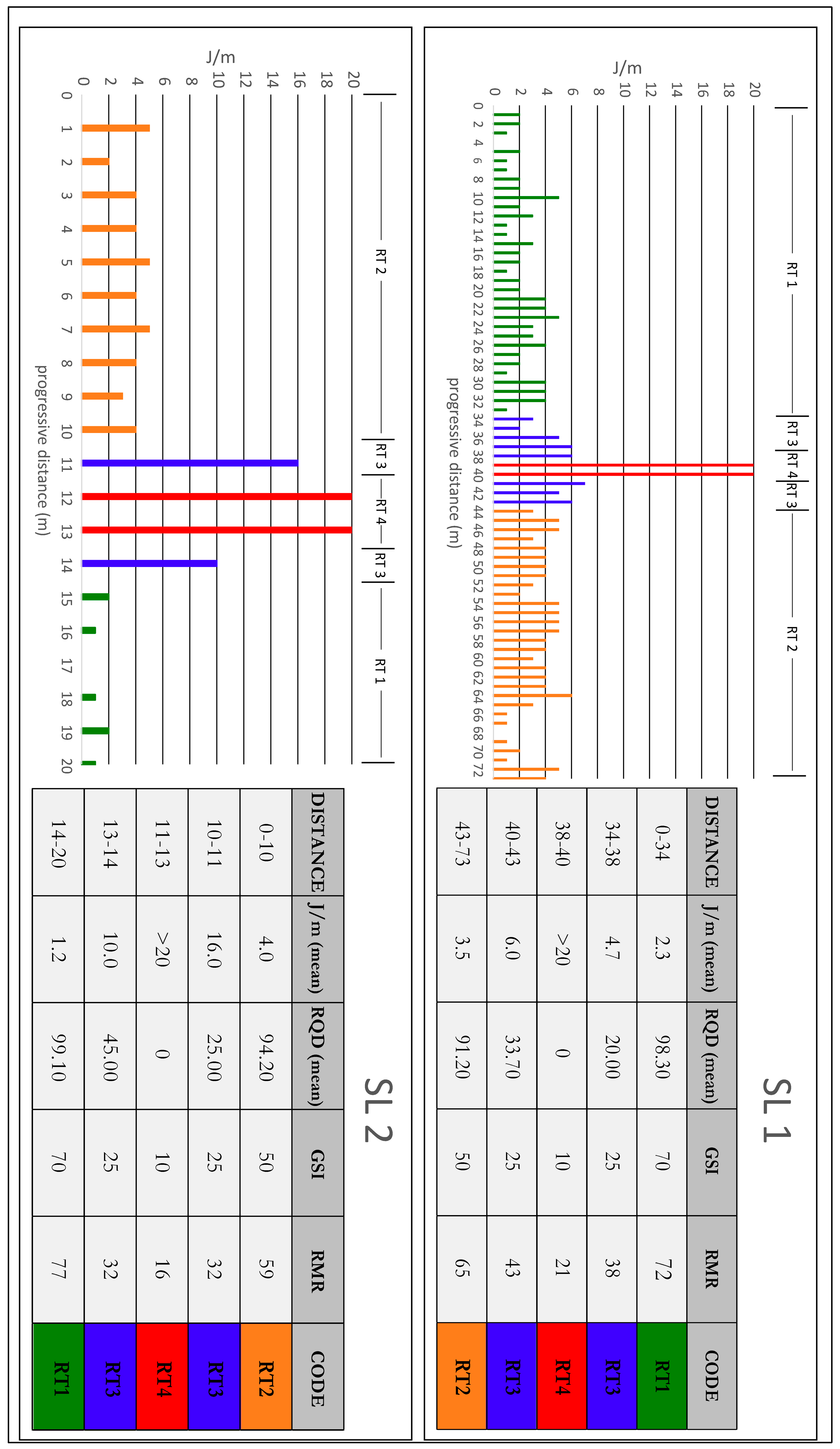
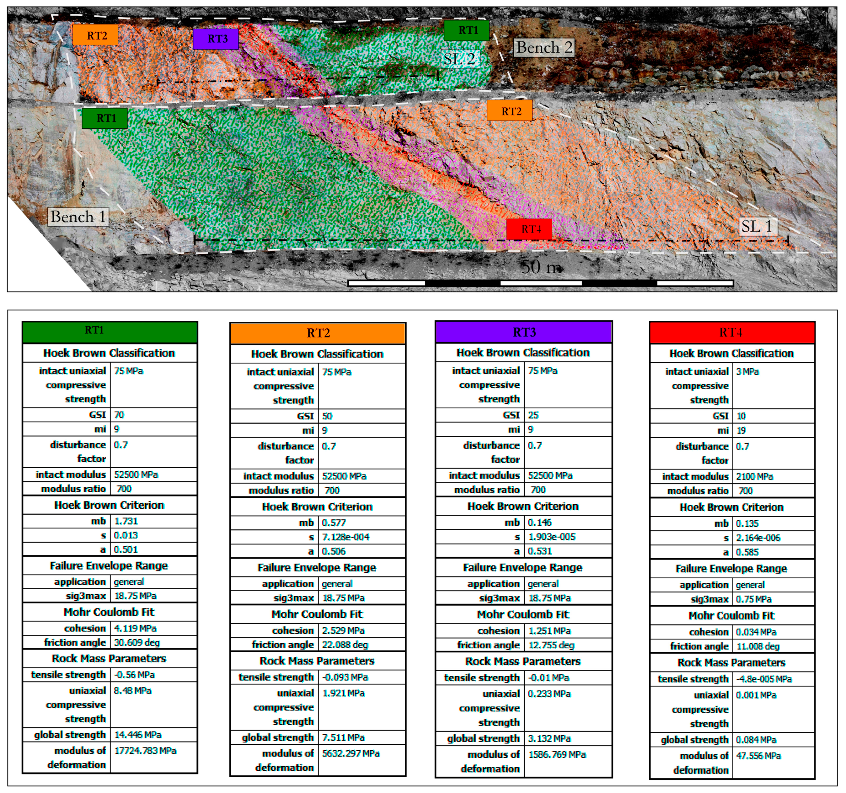
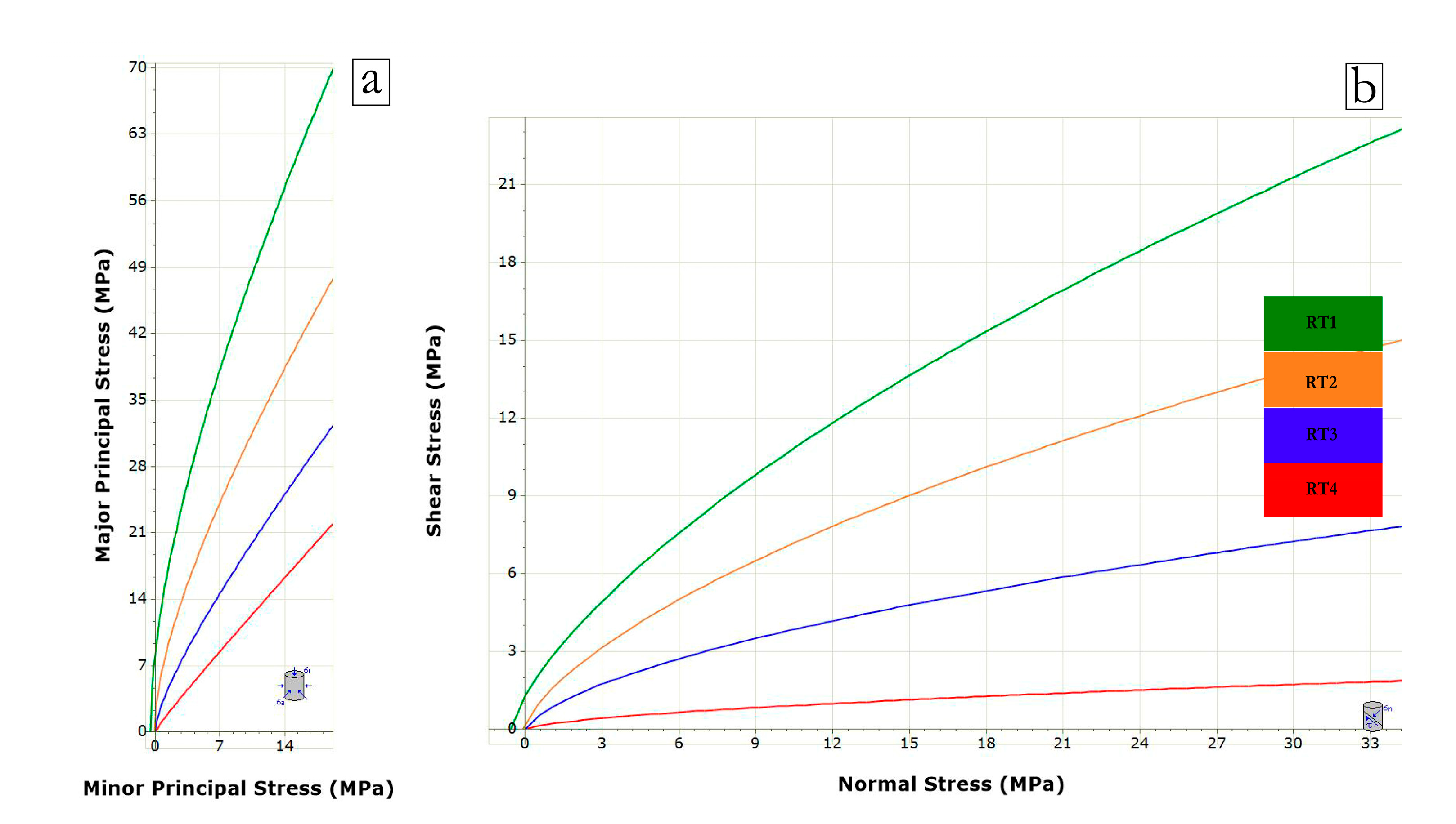
3.1. Geo-Mechanical Surveys

The outcrop was investigated by two geo-mechanical scanlines (SL1 and SL2), 73 and 20 m long, respectively (Figure 3a), according to the ISRM procedures [7]. Data were elaborated aiming at highlighting joint density (number of joints per meter, [J/m]) across the fault zone.
In Figure 3b, the 3D reproduction of the test site is shown. The photogrammetric survey consists of a series of overlapping images acquired with a Canon full frame DSLR coupled with a 50 mm lens. Ground control points for model orientation were dislocated over the quarry front and were acquired by using a rugged GPS tablet (Leica CS25 plus) able to reach a positioning error below 2 cm in the real time RTK mode. MicMac, an open source software, was used to perform tie point extraction, bundle block adjustment, dense image matching, and 3D reconstruction. The obtained cloud consisting of 7.7 million points has been interrogated by means of CloudCompare software for checking structural data using the Compass plugin [34]. A high resolution orthophoto (Figure 3a) with a Ground Sample Distance (GSD) of 1 cm/pixel was produced in order to measure joint spacing in non-reachable portions of the outcrop.

3.2. Infrared Thermography

3.2.1. Principles

Thermography is based on the physical principle stating that, any object having temperature higher than absolute zero, produces electromagnetic radiation. The electromagnetic spectrum is divided arbitrarily into several wavelength regions, called bands, which are distinguished by the methods used to produce and detect the radiation. Thermal radiation occurs in the portion of the spectrum between 0.1 and 100 μm, including parts of the ultraviolet along with visible and infrared regions. However, most of the thermal radiation falls within the IR band [15,35,36]. Thermal cameras for a remote sensing purpose are usually designed and calibrated for the Long-Wavelength IR band (8–14 μm) due to the peak energy emissions for ambient Earth surface temperatures and to the presence of atmospheric windows ([20]). The relation between the total emissive power and an object’s temperature is stated by the Stefan-Bolzmann’s Law [37,38].
W = ε σ T4,
where W, is the total radiant emittance from the body, expressed in Watt m−2, ε is the object emissivity, σ, is the Stephan Boltzmann constant = 5.6697 × 10⁻⁸ Wm−2 K−4, and T is the absolute temperature (expressed in K) of the emitting material.
When a surface is sensed by a thermal camera, the thermal radiation pattern acquired depends not only on the surface temperature but also on the emissivity of the material, on the atmospheric absorption, as well as on the reflection observed on the radiation surface, due to the surrounding bodies [10,39]. These variables must be taken into account at the time of measurement, and their contribution must be known in order to estimate the real temperature of the object.

3.2.2. Surveys Methodology

Two measurement sessions were carried out in 2018 including the first one on January 23 (winter session) and the second one on June 18 (summer session). The aim was to evaluate the behavior of the rock mass in different seasons, insulation conditions, and water content within the fault zone. In every session, a series of thermal images were acquired at an hourly rate. The instrument employed was a FLIR E8 thermal camera (FLIR Systems Inc, [40]) equipped with an uncooled FPA micro bolometer sensor, with a resolution of 320 × 240 pixel, IFOV = 2.6 mrad. It can perform measurements in the thermal infrared band (between 7.5–13 μm). The device was placed on a stable tripod 80 m away from the target, giving a GSD, Ground Sample Distance, of approximatively 0,18 m/pix. In addition to the thermal image, this device produces an optical image, which helps identify the measured area and interpret more easily the obtained thermal data. Thermal data and frames were imported and calibrated by using Flir Tools software (FLIR Systems Inc, version 5.13.17214.2001). After that, the data matrix and optical images were exported to be aligned and to calculate differentials by using the ArcGis Raster Calculator (ESRI ArcMap 10.2.2).
Images were labelled using the following convention: the letter F means the Frame, followed by two numbers identifying the hour when the image was taken, omitting minutes (e.g., F16 refers to an image taken at 16.00 p.m.). During both measuring sessions, the air temperature and humidity were recorded. The first session, conducted from the late morning, allowed for detecting both the heating and the onset of the cooling phase of the rock mass. The air temperature varied between −1 and 11 °C. The second one recorded only the cooling phase of the rock wall, avoiding the contribution of the solar radiation. The measurement session lasted from 19:00 to 23:00, while the air temperature ranged between 24 and 14 °C. In this session, an appreciable run-off flow coming from the top of the quarry front was detected on the Bench 1, steaming from East to West (Left to right in Figure 1 and Figure 3). The temperature of the water flowing was 16.0 °C. The environmental conditions are shown in Table 1.
The emissivity of the rock, the reflected temperature, the shooting length, and the relative humidity have been set appropriately for each shot (except for the winter session, when humidity and reflected temperature were not recorded). In particular, emissivity has been detected by means of lab tests on a rock sample heated in the hoven up to 40 °C. A piece of black electrical tape with a known emissivity of 0.95 was used as a reference, following the “reference emissivity material method” as given in Reference [41]. By assuming emissivity equal to one and by placing a crumpled and re-flattened piece of aluminum foil in front of the camera, the reflected temperature was measured by using the reflector method [42,43]. In particular, the reflector was positioned trying to reproduce the same slope angle and filling the frame. Although outdoor conditions could affect this measure, we consider this approach the one optimizing time saving and accuracy.

3.3. Thermal Conductivity Analysis

Thermal conductivity defines the ability of a material to transfer heat corresponding to the amount of heat transferred from a body per unit area, as it is expressed by the Fourier’s Law of thermal conduction defined using the formula below.
q = λ δ T δ X
where q is the heat flow in the direction of X, and T is the temperature. The coefficient of proportionality λ is the thermal conductivity [43].
A sequence of field and laboratory measures adopting two different methods such as Transient Line Source (TLS, [44]) and Transient Divide Bar (TDB, [43]), was, therefore, carried out on a meaningful number of samples. This is important in order to understand the influence and the accuracy of some experimental conditions, as well as to compare obtained results with known mixing models for measuring bulk thermal conductivity, as proposed in the literature [45].
Aiming at obtaining precise and reliable values of thermal conductivity, density, and porosity parameters were also measured in intact rock specimens. Because of the irregular shapes of the collected samples, bulk density was obtained by water saturation and by weighing all the collected rocks, which refers to Archimede’s Principles [23]. Each specimen was then oven-dried at 70 °C for one day in order to obtain the dry mass and to infer porosity [46].

3.3.1. Transient Line Source (TLS)

K2DPro, which is a thermal property analyzer developed by Decagon Devices, compliant to standards ASTM D5334 and IEEE 442 [47,48] was used. It relies on the Transient Line Source (TLS) method, assuming a heat production at a constant rate by a heated wire and predicting an infinitely long and small source inside an infinite and homogeneous medium.
The obtained temperature, can be found in (Equation (3)).
T 2 T 1 = q 4 π λ · ( ln t 2 ln t 1 ) ,
where q′ (W m−1), is the specific rate at which the heat is generated, T1 and T2 (°C) are the recorded temperatures at time steps t1 and t2 (s), respectively, and λ is the thermal conductivity.
The device uses a specific algorithm based on References [49,50] line heat source analysis. This permits measurements during a heating and a cooling interval, and the separation of the effects of the heat pulse from ambient temperature changes. The algorithm fits time and temperature data using an exponential integral function through a non-linear least squares method. Based on this theory, the K2Dpro device allows for measures with an accuracy of ±10% [47]. It consists of four specific sensors designed for well-defined samples. In this study, the most proper single needle probe (RK-1 sensor, 0 cm long, 3.9 mm diameter) was directly inserted into the investigated materials. With regard to field measures, since thermal conductivity gives a punctual value, two “end members” were tested: sound rock and cataclastic zone. The needle probe was easily introduced in the abundant fine-grained matrix of the cataclastic zone, ensuring a good coupling. Regarding the sound rock, a 4 mm hole was drilled on the surface, and a low quantity of thermal grease was introduced to improve thermal contact between the needle and the rock. Since thermal conductivity is strictly linked to physical, mechanical, and mineralogical characteristics of the material [51,52], laboratory measures both in dry and in wet conditions were conducted too. Due to the difficulty to collect undisturbed samples of the cataclastic fault zone, only sound rock was tested in the laboratory. Each final value achieved is an average over 10 measurements.

3.3.2. Transient Divided Bar (TDB)

The Transient Divided Bar (TDB) is an implemented apparatus designed by Reference [44]. It consists of a stack of two copper blocks acting as a heat sink (the upper one) and a heat source (the lower one), respectively, and, in between the cylindrical rock specimen, is interposed. It is based on Reference [53], adapted for defining thermal conductivity of semiconductors. It predicts that thermal conductivity is obtained through temperature changes between the heat sink and the heat source during the test as well. Temperature changes are recorded and defined by the amount of heat removed from the upper copper block CuΔTu in a specific period of time ΔT, according to the Fourier’s postulate. This is given by (Equation (4)).
C u Δ T u = λ S h t 1 t 2 ( T u T l )   d t
where Cu, is the volume heat capacity (J m−3 K−1) at a constant pressure, ΔTu (°C) is the temperature variation of the upper copper block during a time step dt, λ (W m−1 K−1) is the thermal conductivity of the rock sample, h (m) is the height, S (m2) is the cross-sectional area of the rock sample respectively, T is the temperature, and u and l are suffixes that refer to the upper and lower block. Details of the TDB device as well as the procedure followed to conduct tests, are described in Reference [43]. In particular, TDB is designed for laboratory analysis on sound rocks. For this study, it was applied as a comparative methodology with the TLS apparatus, in order to obtain more reliable thermal conductivity data. Cylindrical specimens 25 ± 0.1 mm in diameter and 20 ± 0.5 mm in thickness, and with parallel, flat (within 0.1 mm) and smooth (within 0.03 mm) surfaces, were prepared. A film of silicone paste (0.1 mm) was applied to improve thermal contact between the rock sample and copper blocks of the used device. Similar to TLS, each final value obtained is averaged over 10 measurements.

4. Results

4.1. Geo-Mechanical Surveys

Bench 1 and 2 are characterized by four main intersecting discontinuity systems (Figure 3a) wich are the schistosity (188/63) and three persistent joint systems, K1, K2, and K3 (respectively, 170/50, 208/79 and 022/81). Fractures are generally closed or with aperture <2 mm while the filling, present as an abundant fraction only in the fault zone, is mostly soft and made of sandy/silty weathered material. No water flows were reported in the winter survey session (probably due to freezing), while a certain humidity degree was present in the summer session. Surface alteration increases approaching to the fault zone. The main geo-structural parameters are summarized in Table 2 and Figure 4.
The number of fractures per linear meter (J/m) provides a good estimate for the potential water circulating through the rock mass. This indicator is consistent with more standardized indexes, such as RQD [54], GSI [55], and RMR [56], as can be seen in Figure 5.
With respect to the Hoek & Brown classification, the GSI value was inferred according to rock mass interlocking and surface conditions, while UCS and mi values were chosen based on an empiric field observation, according to authors’ suggestions [55].
Considering arbitrary joint density thresholds, four lithotechnical units are identified and labelled RT1, RT2, RT3, and RT4, respectively. Quality (latu sensu) of the rock mass decreases from RT1 to RT4 (from Blocky, to Very blocky, to Disturbed to Disintegrated) since the number of joints per meter increases, and RQD, GSI, and RMR decrease.
Figure 5 shows the location of the four litho-technical units on the two surveyed benches. In Figure 6, some geo-mechanical parameters [55] are calculated for every lithotechnical unit, by using the RocData software (Version 5.009, RocScience Inc.) (Figure 7).

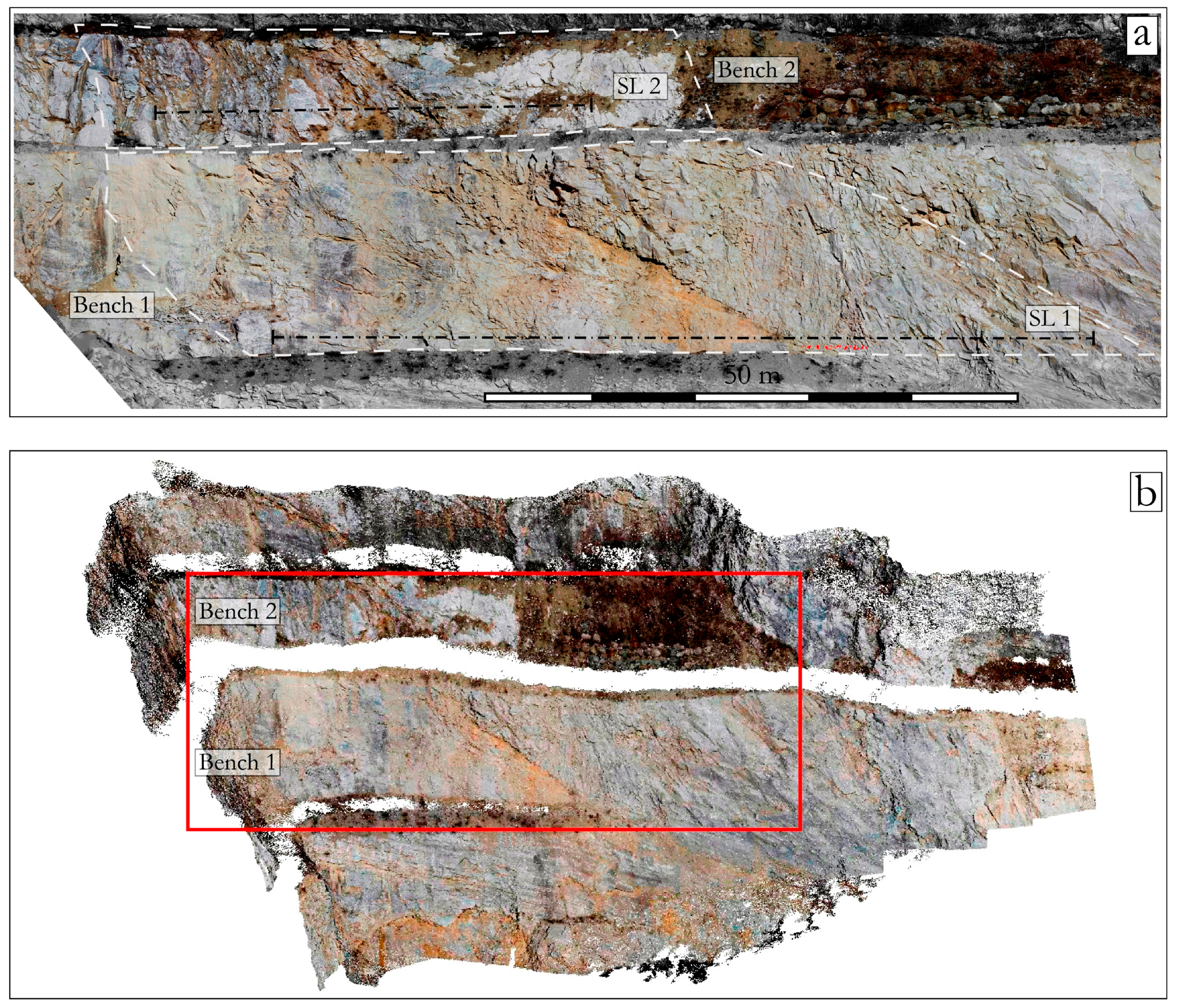
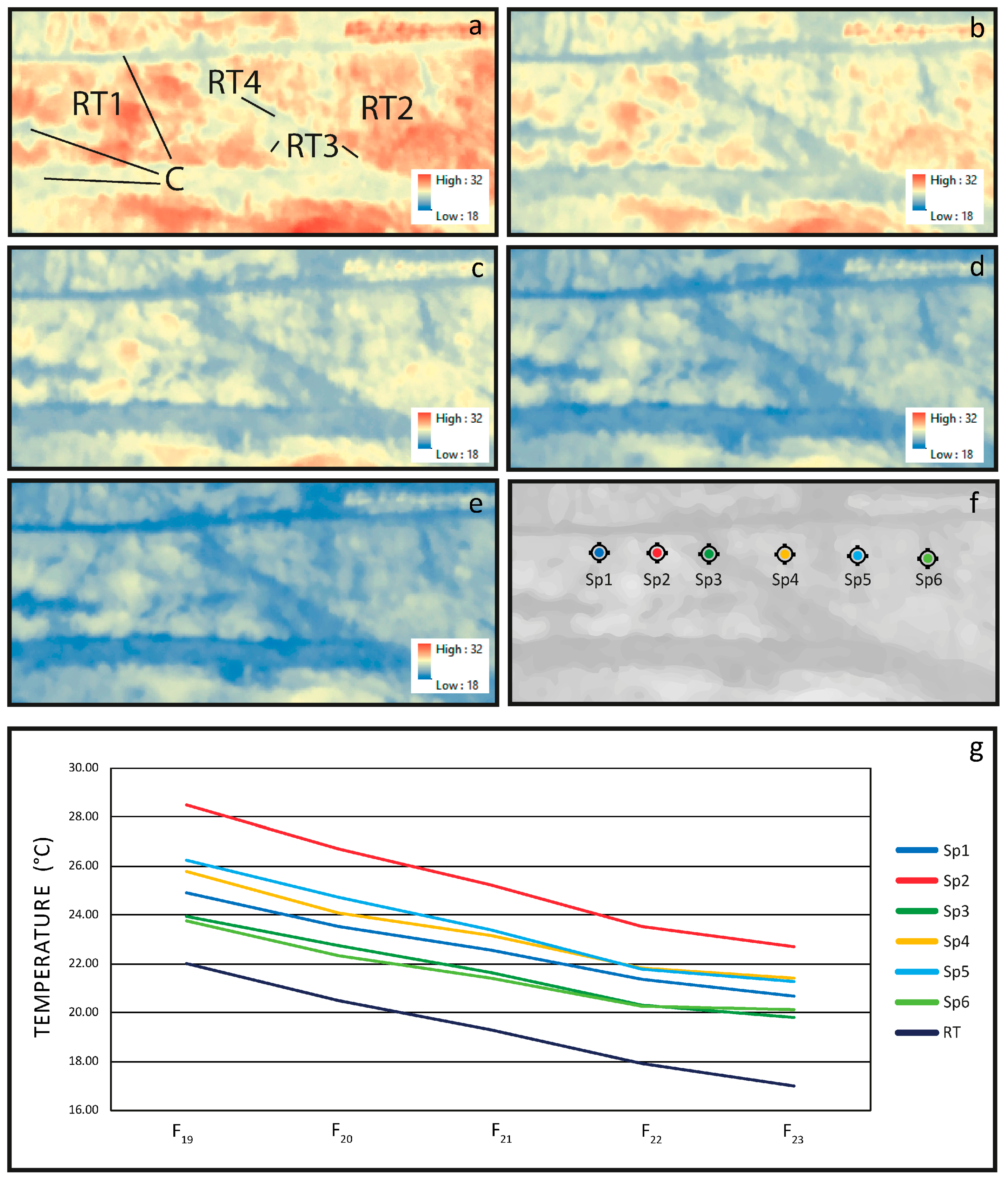
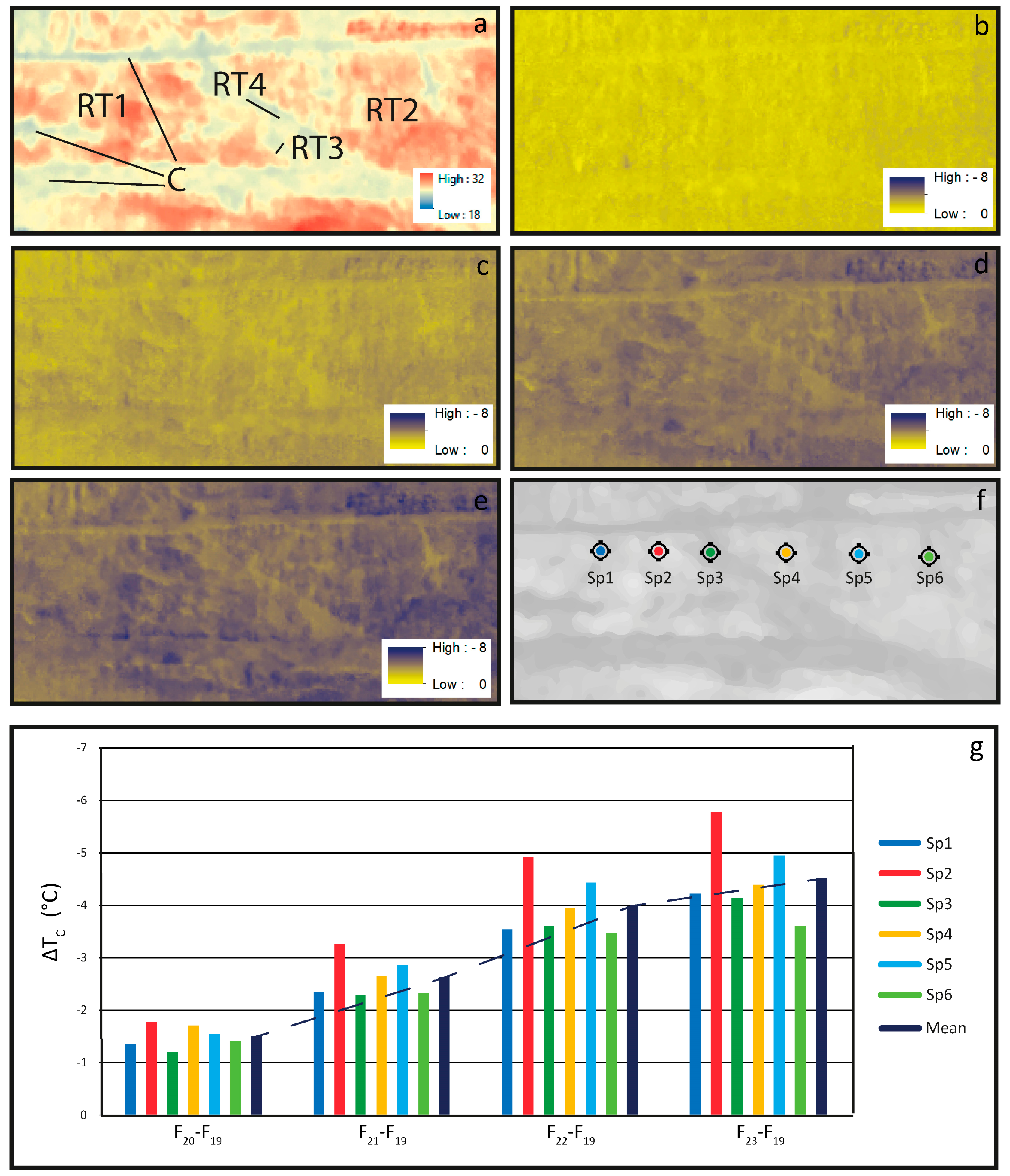
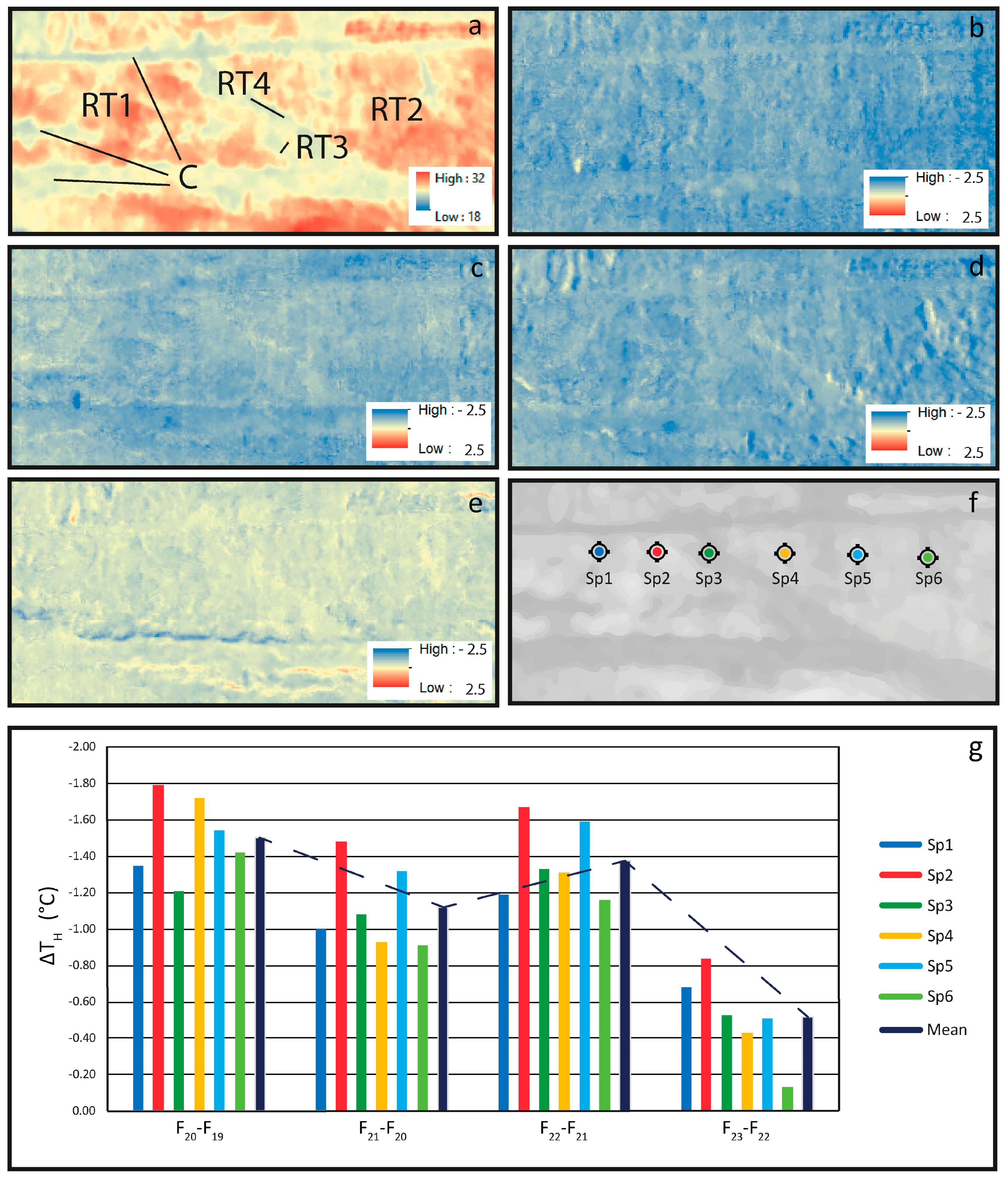
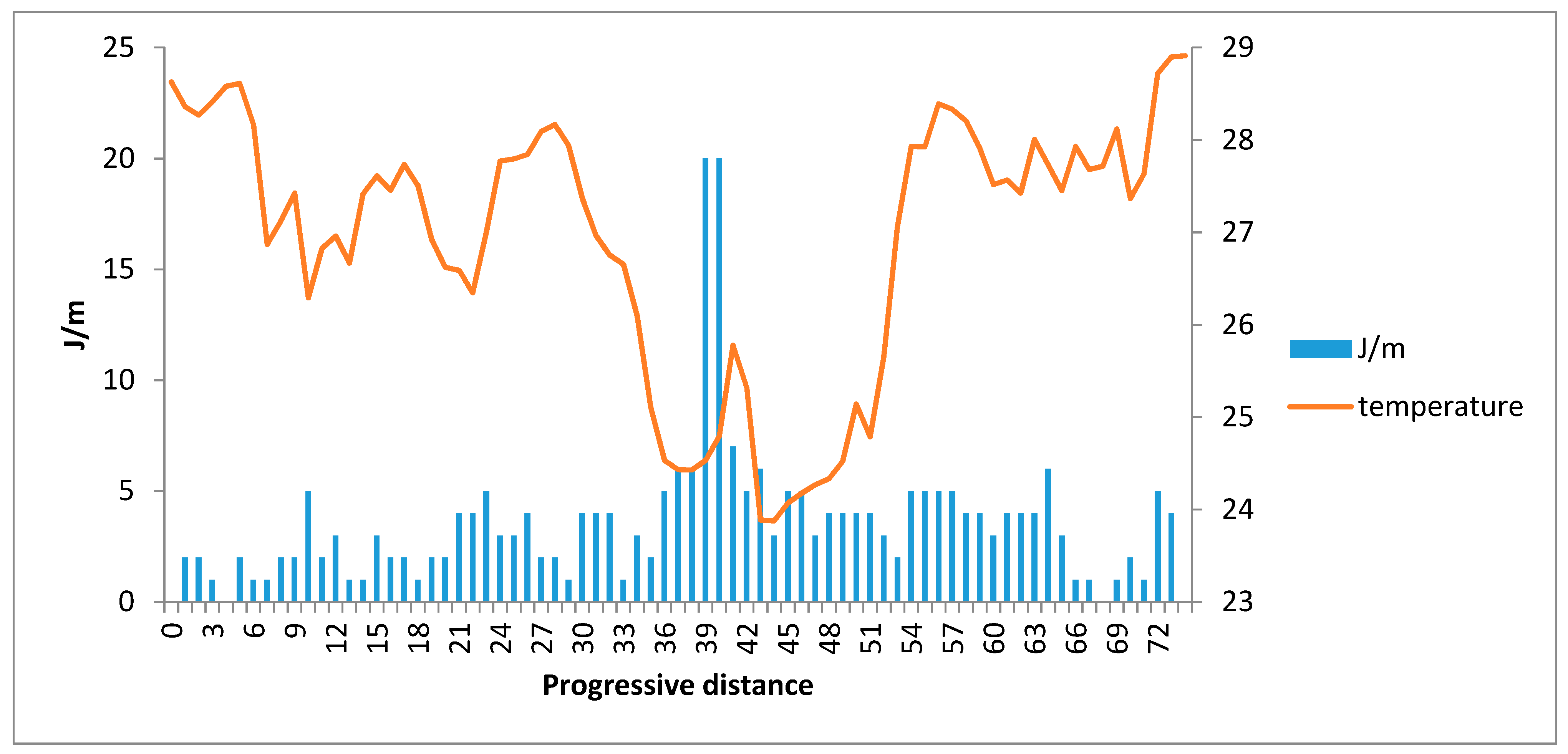
4.2. IRT Winter Field Acquisition

The winter measurement session was conducted from the late morning to the late afternoon on Bench 1. Figure 8 shows raw images and differences between every image and the first one. The solar radiation affects heavily the temperature pattern over the rock outcrop: a quite homogeneous increasing in temperature is shown, with some difference due to the orientation of the surfaces with respect to the position of the sun. For example, the darker loose deposit on the benches (C) has the higher surface temperatures at the start of the survey, and the lower ones at the end. They show a lower thermal inertia than the rocks outcropping in the quarry front. Moreover, it is evident that shaded sectors tend to heat less than the surroundings (cfr. Point S in Figure 8). This is consistent with literature data, which highlights the massive disturbance induced by sun heating [15,17,39]. Only the cooling down phase seems to highlight some peculiar pattern of the fault zone. However, images acquired after the sunset are not enough for providing data necessary for retrieving a cooling rate.

4.3. IRT Summer Field Acquisition

The summer measurement session was conducted entirely after the sun had set, with a decreasing air temperature. An appreciable flow of water (T ~ 16 °C) was present on the top the bench (not visible from the IR camera position due to the presence of the loose deposit), and a certain degree of humidity was visible in the filling of the fault zone fractures.
Looking at the raw images (Figure 9) from a to e (from 19:00 to 23:00), it can be noted that RT1 and RT2 portions are systematic with a higher surface temperature than RT3, RT4, and C portions (loose deposits with vegetation). The temperature trend over time shows an evident decrease, in every sector of the frame. Making some spot measurements (Sp1 to Sp6), it is possible to quantify the cooling rate of the single measurement points along a meaningful profile. The measured points are chosen along a line and include portions of sound rock, wet sectors, and fault rocks. Although a punctual measure may be affected by errors due to tripod instability and camera vibrations, this does not undermine measurement representativeness. Actually, images were aligned before measuring. Furthermore, variations in terms of the temperature of the adjacent pixel are not so significant. The error committed could be regarded as negligible.
Full lines represent the temperature measured at every time step, while the dashed line correspond to the measured air temperature over time. Wet portions (Sp3 and Sp6, detected during the field survey) are characterized by a lower surface temperature in a, and show a lower average cooling rate, with respect to drier ones (Sp1, Sp2, Sp4, and Sp5). Moreover, all the curves tend to have a lower steepness in the right part of the graph, showing a decrease in the cooling rate over time, as illustrated in Figure 9 and Figure 10.
Figure 10 shows thermal differentials of every image compared to the first one, ΔTC. Portions of the bench with different thermal behavior are emphasized. In general, ΔTC between 0 °C and −8 °C are shown over the whole frame. Among the six measured spots, the wet portions (Sp3 and Sp6) have a lower final thermal differential (in e → ΔTC Sp3 ~ −4.0 °C and ΔTC Sp6 ~ −3.5 °C) while the dry rock areas show more consistent thermal losses (e → ΔTC Sp2 ~ −6 °C).
Figure 11 shows thermal differentials between consecutive images ΔTH. In general, hourly variations correspond to ΔTH between −2.5 °C and +0.1 °C. The hourly cooling rate is not constant over time, but generally decreases with a fluctuating trend. This fact could be due to equipment sensitivity, environmental disturbance, and position of the spot measures. In fact, the environmental temperature constantly decreases over time. Wet and dry areas do not show peculiar behavior with respect to this parameter.

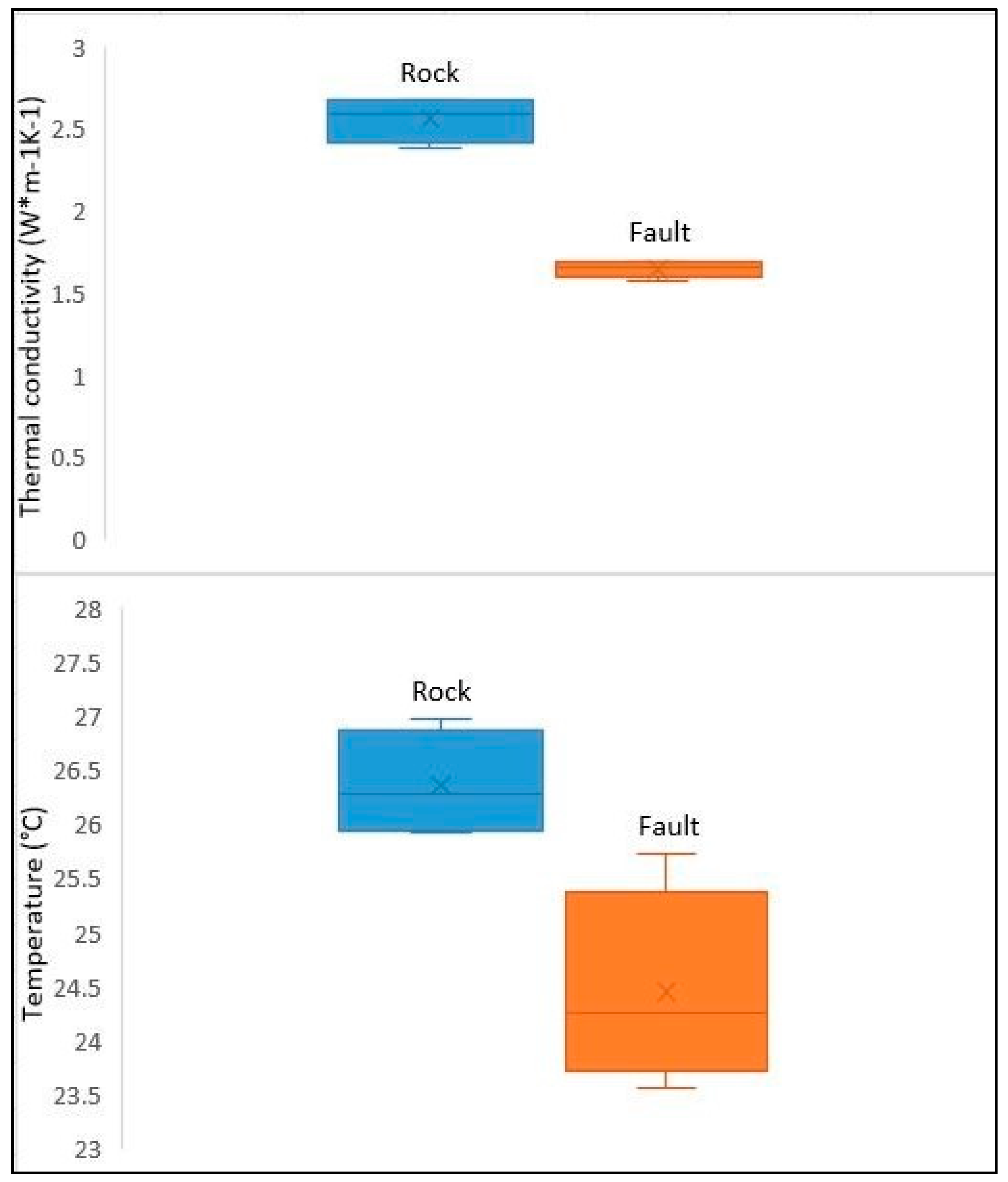
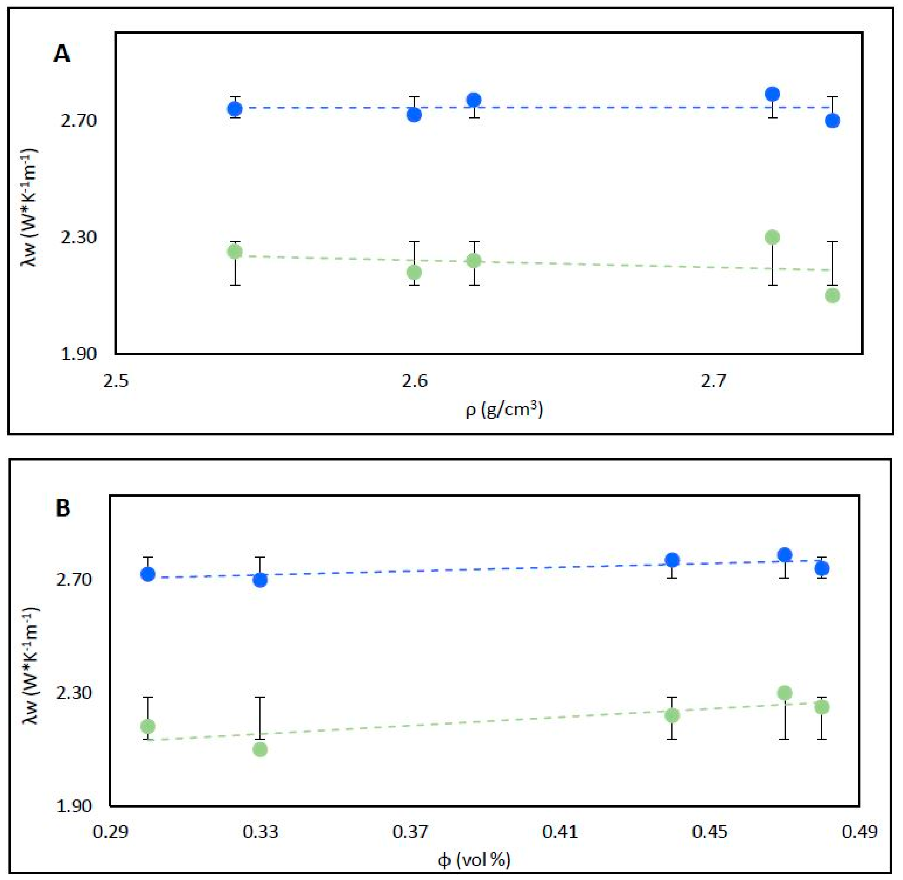
4.4. Thermal Properties

The main results of thermal conductivity, porosity, density, and temperature analysis are summarized in Table 3. The field five measurements on the main representative portion of the sound rock mass (EM1) as well as on the cataclastic zone (EM2) were conducted (Figure 12). Laboratory tests in dry and wet conditions (Table 3) were also performed. In both cases, each test represents an average of five values over 10 measures.
Thermal conductivity measured in the field ranges from 1.58 ÷ 1.69 W m−1K−1 in the EM2 to 2.38 ÷ 2.67 W m−1K−1 for EM1, which shows a difference of about 30 ÷ 40%. At the same time, temperature varies 23.41 ÷ 25.73 °C for EM2 to 25.92 ÷ 26.97 °C for EM1 (Table 3, Figure 13).
On the whole, a general underestimation of TLS than TDB both in dry (TLS: 2.06 to 2.20 W m−1K−1; TDB: 2.67 to 2.72 W m−1K−1) and in wet conditions (TLS: 2.10 to 2.30 W m−1K−1; TDB: 2.70 to 2.77 W m−1K−1), with a maximum of 22.85% and of 22.22% in dry and in wet conditions, respectively, is observed (Table 3, Reference [31]).
Taking into account only the sound rock, if we compare averages values of thermal conductivity for field and laboratory data, the underestimation of TLS with respect to TDB decreases if the TLS technique is used in the field. Moreover, a clear difference of the EM2 with respect to EM1, can be further highlighted. It behaves differently with both TDB and TLS rock data. Moreover, very low standard deviations (0.021 to 0.110) can be observed (Table 3).
Looking at the more representative portions of the sound rock mass, relationships of wet thermal conductivity with porosity (η, vol %) and density (ρ, g/cm3) are summarized in Figure 14.
Density ranges from 2.54 to 2.74 g/cm3 (Figure 14A, Table 3), which are quite high values for a carbonatic rock. Since the negligible porosity (0.30 to 0.48 vol %, Figure 14B, Table 3) and a lack of interconnection between factures, water content does not affect measurements.

5. Discussion

As a general point of view, good agreement between geo-mechanical characteristics of rock masses and their thermophysical behavior is highlighted. Thermal imaging results obtained during rock mass heating and cooling phases, differ in significance depending on several reasons. First of all, the heating trend depends more on the sun position than on the rock mass characteristics. In fact, the relatively uniform and constant slope aspect and surface roughness do not affect substantially thermal measurements.
Then, a reflected and scattered solar radiance play a major role during the day, and considerably affect the rock mass emission term. Thermal contrast between rock mass and air temperature is higher after the sunset. This highlights the rock mass behavior (Figure 8). This is consistent with literature data [15,17]. For those reasons, the results obtained under daylight conditions are affected by a not insignificant source of error.
The summer measurement session, aimed at recording the cooling phase, highlights the different thermal response of the fault zone (RT3 and RT4) with respect to the low fractured sectors (RT1 and RT2). In fact, raw images show that the temperature of the fault zone, characterized by a higher degree of fracturing and low GSI, RQD, and RMR, is sensibly lower in every time step. This outcome is dissimilar from what is obtained in Reference [15]. In fact, authors report higher surface temperature for a high fractured portion of the rock mass. The difference can be ascribed to the hydraulic conditions of the discontinuities. In the case examined herein, there is a consistent water circulation, while, in the reference, the rock mass is in dry conditions. Figure 15 shows the comparison between the number of joint per meter and the measured temperature for the F19 frame on the SL1 scanline (Figure 9a). It is evident that an inverse relationship among these two parameters exist. This is due to the higher water content of RT3 and RT4 units. In fact, while the higher temperature is registered for the sound rock (~32 °C), the water that circulates in fractures at 16 °C cool down the fault zone up to 4 to 5 degrees (F19, Figure 9a). The inverse solution is also possible to apply toward detecting cooler sectors. Thus, the information on the degree of fracturing is possible to retrieve (i.e., SP6, Figure 9).
Hot and dry areas—and, thus, less fractured one—are characterized by a higher cooling rate, while the cold and wet ones (with poor geotechnical characteristics) shows lower temperature differentials. This is in agreement with the Newton’s law of Cooling, stating that the rate of heat loss of a body is directly proportional to the difference in the temperatures between the body and its surroundings.
The sound rock seems to conduct far more than cataclastic fault (in dry conditions), due to the better thermal conductivity values both from field and laboratory surveys (Table 3). This could be due to many factors ranging from different physical, mechanical, and mineralogical characteristics. In particular, lower thermal conductivities of the cataclastic fault zone could be due to a higher content of clay minerals in its matrix or to a higher porosity in dry conditions.
Laboratory experiments were focused on the characterization of the sound rock including comparative and multiple measurements, which allow the obtainment of more reliable values of thermal conductivity through different methodologies and working conditions. In this case, a constant underestimation of TLS data than TDB (Transient Divided Bar technique) for both dry and wet thermal conductivity can be observed. However, this underestimation abruptly decreases when comparing field data on the same rock type. In this case, thermal conductivity using TLS in the field results in higher values, approaching those from the TDB device during laboratory activity. A negligible λwd ratio (ratio between wet and dry thermal conductivity) retrieved in comparative analysis of bulk thermal conductivity of sound rock confirm that porosity does not play an important role in the sampled outcrop. As reported in the literature [57,58,59], fractures can highly increase the λwd ratio, but only when fractures are interconnected and affected by groundwater circulation. On the other hand, some different factors (e.g., air or re-crystallized calcite aggregates or some other low conductive materials fulfilled fractures [60]) can contribute to lowering the λwd ratio even if fractures are abundant in the rock mass. In spite of the very low fracture porosity, the negligible λwd ratio can be ascribed to the mono-mineralic content (around 99.9% volume of Calcite, Carbocalcio Cuneese S.p.A., personal communication), as well. The laboratory tests demonstrate, once more, as the thermal conductivity is strictly connected to the porous medium, the structure and the mineralogy of the rock [61]. Reliability of the obtained results is supported thanks to low standard deviations (Table 3) as well.

6. Conclusions

Both mesoscopic and microscopic characteristics influence thermal properties of the rock masses. The thermal response of an outcrop in heating and in cooling phases, which was confirmed in this study, is caused by different and simultaneous heat transfer processes. At a sample scale, thermal behavior is led by the microscopic features (mineralogical composition, microstructure, interstitial fluid characteristic, etc.) and by the heat conduction process. Thermal conductivity values are systematically higher in the sound rock with respect to the fault zone. A negligible λwd ratio shows that, in this case, fracture porosity is not relevant in influencing thermal properties of the sound rock. Heat conduction is less efficient at the mesoscopic and macroscopic scale, where convection and advection processes due to water circulation into the fracture network are predominant. Thus, the thermal imaging, which highlights a portion of the outcrop characterized by a higher water content, can be a useful tool for detecting a densely fractured litho-technical unit. This can be used when a direct investigation of rock masses (or part of them) is not possible and can be successful in defining portions characterized by similar mechanical and hydro-geological behavior.

Author Contributions

Conceptualization, J.M.C., D.V., and G.M. Methodology, J.M.C. and D.V. Software, D.V. Validation, J.M.C., D.V., and G.M. Formal analysis, J.M.C. Investigation, J.M.C. and D.V. Data curation, J.M.C. and D.V. Writing—original draft preparation, J.M.C. and D.V. Writing—review and editing, J.M.C., D.V., and G.M. Visualization, J.M.C. and D.V. Supervision, G.M. Project administration, G.M. Funding acquisition, G.M.

Funding

This project has received funding from the European Union’s Horizon 2020 research and innovation program under the grant agreement No. 727550.

Acknowledgments

The authors would like to thank the Carbocalcio Cuneese S.p.A. represented by Lorenzo Callegaro, for his willingness in giving all the needful data about the geological and hydrogeological conditions of the quarry area, as well as for allowing the field surveys at the quarry over four different periods. Federico Vagnon is also warmly thanked for the density and porosity analysis on collected samples.

Conflicts of Interest

The authors declare no conflict of interest.

References

  1. Dochez, S.; Laouafa, F.; Franck, C.; Guedon, S.; Martineau, F.; Bost, M.; D’Amato, J. Influence of Water on Rock Discontinuities and Stability of Rock Mass. Procedia Earth Planet. Sci. 2013, 7, 219–222. [Google Scholar] [CrossRef] [Green Version]
  2. Iverson, R.M. Landslide triggering by rain infiltration. Water Resour. Res. 2000, 36, 1897–1910. [Google Scholar] [CrossRef] [Green Version]
  3. Price, J. Implications of groundwater behaviour on the geomechanics of rock slope stability. In Proceedings of the APSSIM 2016, Brisbane, Australia, 6–8 September 2016. [Google Scholar]
  4. Covington, M.D.; Luhmann, A.J.; Gabrovšek, F.; Saar, M.O.; Wicks, C.M. Mechanisms of heat exchange between water and rock in karst conduits: HEAT TRANSPORT IN KARST. Water Resour. Res. 2011, 47, 1897–1910. [Google Scholar] [CrossRef]
  5. Zhang, W.; Yang, H.; Lu, L.; Fang, Z. Investigation on the heat transfer of energy piles with two-dimensional groundwater flow. Int. J. Low-Carbon Technol. 2015, 12, 43–50. [Google Scholar] [CrossRef] [Green Version]
  6. Sheets, R.A.; Burns, E.R. Geothermal Heating and Cooling—The Role of Groundwater. Available online: http://wmao.org/wmao/wp-content/uploads/2014/04/Water-Table-Spring-2014-Issue.pdf (accessed on 18 January 2019).
  7. Suggested Methods for the Quantitative Description of Discontinuities in Rock Masses 1978. Available online: https://www.researchgate.net/publication/313659691_Suggested_methods_for_the_quantitative_description_of_discontinuities_in_rock_masses_International_Society_for_Rock_Mechanics (accessed on 18 January 2019).
  8. Balaras, C.A.; Argiriou, A.A. Infrared thermography for building diagnostics. Energy Build. 2002, 34, 171–183. [Google Scholar] [CrossRef]
  9. Nolesini, T.; Frodella, W.; Bianchini, S.; Casagli, N. Detecting Slope and Urban Potential Unstable Areas by Means of Multi-Platform Remote Sensing Techniques: The Volterra (Italy) Case Study. Remote Sens. 2016, 8, 746. [Google Scholar] [CrossRef]
  10. Spampinato, L.; Calvari, S.; Oppenheimer, C.; Boschi, E. Volcano surveillance using infrared cameras. Earth-Sci. Rev. 2011, 106, 63–91. [Google Scholar] [CrossRef]
  11. Coppola, D.; Staudacher, T.; Cigolini, C. Field thermal monitoring during the August 2003 eruption at Piton de la Fournaise (La Réunion). J. Geophys. Res. 2007, 112. [Google Scholar] [CrossRef] [Green Version]
  12. Furukawa, Y. Infrared thermography of the fumarole area in the active crater of the Aso volcano, Japan, using a consumer digital camera. J. Asian Earth Sci. 2010, 38, 283–288. [Google Scholar] [CrossRef] [Green Version]
  13. Stevenson, J.A.; Nick, V. Fumarole monitoring with a handheld infrared camera: Volcán de Colima, Mexico, 2006–2007. J. Volcanol. Geotherm. Res. 2008, 177, 911–924. [Google Scholar] [CrossRef]
  14. Tonelli, A. Some operative applications of remote sensing. Ann. Geophys. 2000, 43, 1177–1196. [Google Scholar]
  15. Pappalardo, G.; Mineo, S.; Zampelli, S.P.; Cubito, A.; Calcaterra, D. InfraRed Thermography proposed for the estimation of the Cooling Rate Index in the remote survey of rock masses. Int. J. Rock Mech. Min. Sci. 2016, 83, 182–196. [Google Scholar] [CrossRef]
  16. Fiorucci, M.; Marmoni, G.M.; Martino, S.; Mazzanti, P. Thermal Response of Jointed Rock Masses Inferred from Infrared Thermographic Surveying (Acuto Test-Site, Italy). Sensors 2018, 18, 2221. [Google Scholar] [CrossRef] [PubMed]
  17. Baroň, I.; Bečkovský, D.; Míča, L. Application of infrared thermography for mapping open fractures in deep-seated rockslides and unstable cliffs. Landslides 2014, 11, 15–27. [Google Scholar] [CrossRef]
  18. Mineo, S.; Pappalardo, G.; Rapisarda, F.; Cubito, A.; Di Maria, G. Integrated geostructural, seismic and infrared thermography surveys for the study of an unstable rock slope in the Peloritani Chain (NE Sicily). Eng. Geol. 2015, 195, 225–235. [Google Scholar] [CrossRef]
  19. Gigli, G.; Frodella, W.; Garfagnoli, F.; Morelli, S.; Mugnai, F.; Menna, F.; Casagli, N. 3-D geomechanical rock mass characterization for the evaluation of rockslide susceptibility scenarios. Landslides 2014, 11, 131–140. [Google Scholar] [CrossRef]
  20. Frodella, W.; Gigli, G.; Morelli, S.; Lombardi, L.; Casagli, N. Landslide Mapping and Characterization through Infrared Thermography (IRT): Suggestions for a Methodological Approach from Some Case Studies. Remote Sens. 2017, 9, 1281. [Google Scholar] [CrossRef]
  21. Pappalardo, G.; Mineo, S.; Angrisani, A.C.; Di Martire, D.; Calcaterra, D. Combining field data with infrared thermography and DInSAR surveys to evaluate the activity of landslides: the case study of Randazzo Landslide (NE Sicily). Landslides 2018, 11, 2173–2193. [Google Scholar] [CrossRef]
  22. Brooks, A.L.; Zhou, H.; Hanna, D. Comparative study of the mechanical and thermal properties of lightweight cementitious composites. Constr. Build. Mater. 2018, 159, 316–328. [Google Scholar] [CrossRef]
  23. Balandin, A.A. The Heat Is On: Graphene Applications. IEEE Nanotechnol. Mag. 2011, 5, 15–19. [Google Scholar] [CrossRef]
  24. Jafari, N.S.J. A review on modeling of the thermal conductivity of polymeric nanocomposites. E-Polym. 2012, 12. [Google Scholar] [CrossRef]
  25. Gomez-Mares, M.; Tugnoli, A.; Landucci, G.; Cozzani, V. Performance Assessment of Passive Fire Protection Materials. Ind. Eng. Chem. Res. 2012, 51, 7679–7689. [Google Scholar] [CrossRef]
  26. Albert, K.; Schulze, M.; Franz, C.; Koenigsdorff, R.; Zosseder, K. Thermal conductivity estimation model considering the effect of water saturation explaining the heterogeneity of rock thermal conductivity. Geothermics 2017, 66, 1–12. [Google Scholar] [CrossRef]
  27. Feng, J.; Gao, Z.; Zhu, R.; Luo, Z.; Zhang, L. The application of thermal conductivity measurements to the Kuqa River profile, China, and implications for petrochemical generation. SpringerPlus 2013, 2. [Google Scholar] [CrossRef]
  28. Hartmann, A.; Pechnig, R.; Clauser, C. Petrophysical analysis of regional-scale thermal properties for improved simulations of geothermal installations and basin-scale heat and fluid flow. Int. J. Earth Sci. 2008, 97, 421–433. [Google Scholar] [CrossRef]
  29. Jorand, R.; Fehr, A.; Koch, A.; Clauser, C. Study of the variation of thermal conductivity with water saturation using nuclear magnetic resonance. J. Geophys. Res. Solid Earth 2011, 116. [Google Scholar] [CrossRef] [Green Version]
  30. Ramstad, R.K.; Midttømme, K.; Liebel, H.T.; Frengstad, B.S.; Willemoes-Wissing, B. Thermal conductivity map of the Oslo region based on thermal diffusivity measurements of rock core samples. Bull. Eng. Geol. Environ. 2015, 74, 1275–1286. [Google Scholar] [CrossRef]
  31. Fuchs, S.; Förster, A. Rock thermal conductivity of Mesozoic geothermal aquifers in the Northeast German Basin. Chem. Erde-Geochem. 2010, 70, 13–22. [Google Scholar] [CrossRef] [Green Version]
  32. Norden, B.; Förster, A.; Balling, N. Heat flow and lithospheric thermal regime in the Northeast German Basin. Tectonophysics 2008, 460, 215–229. [Google Scholar] [CrossRef] [Green Version]
  33. Barale, L.; Bertok, C.; d’Atri, A.; Martire, L.; Piana, F.; Domini, G. Geology of the Entracque—Colle di Tenda area (Maritime Alps, NW Italy). J. Maps 2016, 12, 359–370. [Google Scholar] [CrossRef]
  34. Thiele, S.T.; Grose, L.; Samsu, A.; Micklethwaite, S.; Vollgger, S.A.; Cruden, A.R. Rapid, semi-automatic fracture and contact mapping for point clouds, images and geophysical data. Solid Earth 2017, 8, 1241–1253. [Google Scholar] [CrossRef] [Green Version]
  35. Lillesand, T.M.; Kiefer, R.W.; Chipman, J.W. Remote Sensing and Image Interpretation, 5th ed.; Wiley: New York, NY, USA, 2004. [Google Scholar]
  36. Maldague, X.P.V. Nondestructive Evaluation of Materials by Infrared Thermography; Springer London: London, UK, 1993. [Google Scholar]
  37. Boltzmann, L. Ableitung des Stefan’schen Gesetzes, betreffend die Abhängigkeit der Wärmestrahlung von der Temperatur aus der electromagnetischen Lichttheorie. Ann. Phys. 1884, 258, 291–294. [Google Scholar] [CrossRef]
  38. Stefan, J. Über die Beziehung zwischen der Wärmestrahlung und der Temperatur. Sitzungsberichte Math.-Naturwissenschaftlichen Cl. Kais. Akad. Wiss. Ger. 1879, 79, 391–428. [Google Scholar]
  39. Teza, G.; Marcato, G.; Castelli, E.; Galgaro, A. IRTROCK: A MATLAB toolbox for contactless recognition of surface and shallow weakness of a rock cliff by infrared thermography. Comput. Geosci. 2012, 45, 109–118. [Google Scholar] [CrossRef]
  40. FLIR Systems, Thermography Product Catalog. Publ. No. T559480. Available online: https://www.ien.eu/uploads/tx_etim/43591_flir.pdf 2013 (accessed on 18 January 2019).
  41. ISO 18434-1:2008 Condition Monitoring and Diagnostics of Machines -- Thermography -- Part 1: General procedures. Available online: https://www.iso.org/standard/41648.html (accessed on 18 January 2019).
  42. ASTM E1862-97e1. Standard Test Methods for Measuring and Compensating for Reflected Apparent Temperature Using Infrared Imaging Radiometers; ASTM: West Conshohocken, PA, USA, 1997. [Google Scholar]
  43. Pasquale, V.; Verdoya, M.; Chiozzi, P. Measurements of rock thermal conductivity with a Transient Divided Bar. Geothermics 2015, 53, 183–189. [Google Scholar] [CrossRef]
  44. Transient Plane and Line Source Methods for Soil Thermal Conductivity. Transient Plane Line Source Methods Soil Therm. Available online: https://www.researchgate.net/publication/319337593_Transient_Plane_and_Line_Source_Methods_for_Soil_Thermal_Conductivity (accessed on 18 January 2019).
  45. Fuchs, S.; Schütz, F.; Förster, H.-J.; Förster, A. Evaluation of common mixing models for calculating bulk thermal conductivity of sedimentary rocks: Correction charts and new conversion equations. Geothermics 2013, 47, 40–52. [Google Scholar] [CrossRef] [Green Version]
  46. Franklin, J.A.; Vogler, U.W.; Szlavin, J.; Edmond, J.M.; Bieniawski, Z.T. ISRM—Suggested methods for determining water-content, porosity, density, absorption and related properties and swelling and slake-durability index properties. In The Complete ISRM Suggested Methods for Rock Characterization, Testing and Monitoring:1974-2006 ISRM Turkish National Group; E ISRM: Ankara, Turkey, 2007. [Google Scholar]
  47. ASTM D5334—Standard Test Method for Determination of Thermal Conductivity of Soil and Soft Rock by Thermal Needle Probe Procedure; ASTM: West Conshohocken, PA, USA, 2014.
  48. IEEE 442-1981—IEEE Guide for Soil Thermal Resistivity Measurements. C25W/P442_WG—Working Group for Guide for Soil Thermal Resistivity Measurements—IEEE 442 1981. Available online: https://global.ihs.com/doc_detail.cfm?document_name=IEEE%20442&item_s_key=00036135&csf=TIA (accessed on 18 January 2019).
  49. Carslaw, H.S.; Jaeger, J.C. Conduction of Heat in Solids; Oxford Science Publications: Oxford, UK, 1959. [Google Scholar]
  50. Kluitenberg, G.J.; Ham, J.M.; Bristow, K.L. Error Analysis of the Heat Pulse Method for Measuring Soil Volumetric Heat Capacity. Soil Sci. Soc. Am. J. 1993, 57, 1444–1451. [Google Scholar] [CrossRef]
  51. Yaşar, E.; Erdoğan, Y.; Güneyli, H. Determination of the thermal conductivity from physico-mechanical properties. Bull. Eng. Geol. Environ. 2008, 67, 219–225. [Google Scholar] [CrossRef]
  52. Pribnow, D.; Umsonst, T. Estimation of thermal conductivity from the mineral composition: Influence of fabric and anisotropy. Geophys. Res. Lett. 1993. [Google Scholar] [CrossRef]
  53. Joffé, A.F. Heat transfer in semiconductors. Can. J. Phys. 1956, 34, 1342–1355. [Google Scholar] [CrossRef]
  54. Deere, D.U.; Hendron, A.J.; Patton, F.D.; Cording, E.J. Design of Surface and Near-Surface Construction in Rock; American Rock Mechanics Association: Alexandria, VA, USA, 1966; Available online: https://www.onepetro.org/conference-paper/ARMA-66-0237 (accessed on 18 January 2019).
  55. Hoek, E.; Carranza-Torres, C.; Corkum, B. HOEK-BROWN FAILURE CRITERION—2002 EDITION. In Proceedings of the Fifth North American Rock Mechanics Symposium, Toronto, ON, Canada, 7–10 July 2002; pp. 267–273. [Google Scholar]
  56. Bieniawski, Z.T. Engineering Rock Mass Classifications: A Complete Manual for Engineers and Geologists in Mining, Civil, and Petroleum Engineering; Wiley: New York, NY, USA, 1989. [Google Scholar]
  57. Popov, Y.; Tertychnyi, V.; Romushkevich, R.; Korobkov, D.; Pohl, J. Interrelations Between Thermal Conductivity and Other Physical Properties of Rocks: Experimental Data. Pure Appl Geophys 2003, 160, 1137–1161. [Google Scholar] [CrossRef]
  58. Moh’d, B.K. Compressive Strength of Vuggy Oolitic Limestones as a Function of Their Porosity and Sound Propagation. Jordan J. Earth Environ. Sci. 2009, 2, 18–25. [Google Scholar]
  59. Bagrintseva, K.I. Carbonate Reservoir Rocks; John Wiley & Sons, Inc.: Hoboken, NJ, USA, 2015. [Google Scholar]
  60. Horai, K.; Simmons, G. Thermal conductivity of rock-forming minerals. Earth Planet. Sci. Lett. 1969, 6, 359–368. [Google Scholar]
  61. Surma, F.; Geraud, Y. Porosity and Thermal Conductivity of the Soultz-sous-Forêts Granite. Pure Appl. Geophys. 2003, 160, 1125–1136. [Google Scholar] [CrossRef]
Figure 1. Overall perspective of the test site.
Remotesensing 11 00179 g001
Figure 2. Location and geological map of the test site. Legend: 1—Slope and talus debris. 2—Undifferentiated glacial deposits. 3—Carnieules. 4—Puriac Limestone. 5—Marne Nere. 6—Lausa Limestone. 7—Entracque marl. Completed and modified after Reference [33].
Remotesensing 11 00179 g002
Figure 3. Details of the study area. (a): orthomosaic. (b): Image of the dense cloud reconstructed using MicMac software. In the red box is the surveyed area.
Remotesensing 11 00179 g003
Figure 4. Stereoplot reporting the poles of the main discontinuity sets (S, K1, K2, K3) and the great circles of the front (Black) and fault plane (Blue).
Remotesensing 11 00179 g004
Figure 5. Scanlines results on the selected benches: rock types (in colours) and geomechanical indexes are referred to faults and the surroundings.
Remotesensing 11 00179 g005
Figure 6. Rock mechanics field characterization for the four identified litho-technical units.
Remotesensing 11 00179 g006
Figure 7. Principal stress plot (a) and Normal vs. Shear stress plot (b) for the four litho-technical units, after the Hoek-Brown criterion.
Remotesensing 11 00179 g007
Figure 8. Winter measurement session, raw images, and thermal differentials.
Remotesensing 11 00179 g008
Figure 9. Summer measurement session (a) = image at 19:00 (F19), (b) = image at 20:00 (F20), (c) = image at 21:00 (F21), (d) = image at 22:00 (F22), (e) = image at 23:00 (F23), (f) = position of measurement points, and (g) = temperature trends of the spot measurement points. RT stands for the ambient temperature.
Remotesensing 11 00179 g009
Figure 10. Summer measurement session (a) = image at 19:00 (F19), (b) = F20-F19, (c) = F21-F19, (d) = F22-F19, (e) = F23-F19, (f) = position of measurement points, and (g) = temperature differentials of the spot measurement points.
Remotesensing 11 00179 g010
Figure 11. Summer measurement session 1-hour thermal differentials ΔTH. (a) = image at 19:00 (F19), (b) = F20-F19, (c) = F21-F20, (d) = F22-F21, (e) = F23-F22, (f) = position of measurement points, and (g) temperature differentials of the spot measurement points.
Remotesensing 11 00179 g011
Figure 12. Specimen location for thermal conductivity measurements. EM 1: sound rock. EM2: cataclastic zone.
Remotesensing 11 00179 g012
Figure 13. Field data relative to thermal conductivity (above) and temperature (below) both for cataclastic fault zone (Orange) and low fractured rock mass (Blue). Estimated errors in the measurement are represented by vertical error bars.
Remotesensing 11 00179 g013
Figure 14. Wet thermal conductivity (λw, W*K−1m−1) from TLS (green circles) and TDB methods (blue circles) vs. density (ρ, g/cm3) in (A), and porosity (φ, vol %) in (B), respectively. Error bars represent standard deviation.
Remotesensing 11 00179 g014
Figure 15. Comparison between the number of joints per meter and the measured temperature for the F19 frame on the SL1 scanline.
Remotesensing 11 00179 g015
Table 1. Environmental conditions at survey time.
Winter SessionSummer Session
Data23 January 201818 June 2018
Start–End Time11:40 ÷ 18:0719:00 ÷ 23:00
Sunrise–Sunset7:58 ÷ 17:275:46 ÷ 21:17
Direct Insolation (start ÷ end)10:30 ÷ 16:30-- ÷ 18:50
Air Temperature−1 °C ÷ +11 °C+14 °C ÷ +24 °C
H2O Temperatureno water~ 16 °C
Air Humiditynot measured55% ÷ 60%
Shooting Length 80 m80 m
Emissivity0.950.95
Reflected Temperaturenot measured18°C ÷ 22 °C
Table 2. Main geo-mechanical features from the surveys.
SetSpacing (mm)Persistence (m)RoughnessApertureInfillingWeatheringGroundwater
S200 ÷ 6003 ÷ 10roughclosednoneslightdry to damp
K140 ÷ 2003 ÷ 10roughclosed to partly opennone-softnone to slightdry to damp
K260 ÷ 6003 ÷ 10roughclosed to tightnone-softnone to slightdry to damp
K340 ÷ 2003 ÷ 10roughclosed to tightnone-softnone to slightdry to damp
Table 3. Results from field and laboratory activities. Keys: TLS (Transient Line Source methods) and TDB (Transient Divided Bar technique), EM2 and EM1, fault and rock respectively. The symbol percentage indicates the percentage between two measurements of thermal conductivity. T is the temperature (°C), φ indicates the porosity (% vol), and ρ defines density (g/cm3). λb, is the bulk of thermal conductivity (W m−1K−1). St.dev., the standard deviation of λb.
TestFieldLab DryLab WetOther Properties
TLSEM2TLSEM1% EM2vsEM1TDBEM1TLEM1% TDBvsTLSTDBEM1TLSEM1% TDBvsTLSφρTEM1TEM2
11.692.5333.202.672.0622.852.702.1022.220.332.6226.9725.73
21.682.3829.412.712.1520.662.772.2219.860.442.7426.5324.30
31.632.6739.952.722.2019.122.772.3017.560.472.7226.0223.41
41.582.639.232.682.0722.762.722.2517.880.482.5425.9223.56
51.582.639.232.692.1320.822.722.1819.850.302.6026.2924.20
λb1.6322.556 2.6942.122 2.7442.210
St. dev.0.0530.110 0.0210.058 0.0360.075

