Article

Soil Moisture Monitoring Using Remote Sensing Data and a Stepwise-Cluster Prediction Model: The Case of Upper Blue Nile Basin, Ethiopia

1
Remote Sensing Research and Development Department, EORC, Ethiopian Space Science & Technology Institute, Addis Ababa 33679, Ethiopia
2
Institute of Land Administration, Bahir Dar University, Bahir Dar 79, Ethiopia
3
National Drought Mitigation Center, University of Nebraska-Lincoln, Lincoln, NE 830988, USA
4
Department of Geography and Environmental Studies, Bahir Dar University, Bahir Dar 79, Ethiopia
*
Author to whom correspondence should be addressed.
Remote Sens. 2019, 11(2), 125; https://doi.org/10.3390/rs11020125
Submission received: 2 November 2018 / Revised: 12 December 2018 / Accepted: 4 January 2019 / Published: 10 January 2019
(This article belongs to the Special Issue Remote Sensing of Drought Monitoring)

Abstract

:
In this study, a residual soil moisture prediction model was developed using the stepwise cluster analysis (SCA) and model prediction approach in the Upper Blue Nile basin. The SCA has the advantage of capturing the nonlinear relationships between remote sensing variables and volumetric soil moisture. The principle of SCA is to generate a set of prediction cluster trees based on a series of cutting and merging process according to a given statistical criterion. The proposed model incorporates the combinations of dual-polarized Sentinel-1 SAR data, normalized difference vegetation index (NDVI), and digital elevation model as input parameters. In this regard, two separate stepwise cluster models were developed using volumetric soil moisture obtained from automatic weather stations (AWS) and Noah model simulation as response variables. The performance of the SCA models have been verified for different significance levels (i.e., α = 0.01 , α = 0.05 , and α = 0.1 ). Thus, the AWS based SCA model with α = 0.05 was found to be an optimal model for predicting volumetric residual soil moisture, with correlation coefficient (r) values of 0. 95 and 0.87 and root mean square error (RMSE) of 0.032 and 0.097 m3/m3 during the training and testing periods, respectively. While in the case of the Noah SCA model an optimal prediction performance was observed when α value was set to 0.01, with r being 0.93 and 0.87 and RMSE of 0.043 and 0.058 m3/m3 using the training and testing datasets, respectively. In addition, our result indicated that the combined use of Sentinel-SAR data and ancillary remote sensing products such as NDVI could allow for better soil moisture prediction. Compared to the support vector regression (SVR) method, SCA shows better fitting and prediction accuracy of soil moisture. Generally, this study asserts that the SCA can be used as an alternative method for remote sensing based soil moisture predictions.

1. Introduction

Soil moisture is a critical component of agricultural development because its availability and distribution substantially determine the growth and productivity of crops. Soil moisture is one of the limiting factors in countries such as Ethiopia where the country is predominantly affected by recurrent drought and dependent on rain-fed farming practices [1]. Ethiopia’s crop production and productivity are low and dominated by smallholder farmers [2]. Most of these farmers are unable to sustain their livelihoods by a single harvest during the main rainy season [3,4]. More specifically, the Upper Blue Nile (UBN) basin of Ethiopia receives an adequate amount of rainfall (>2000 mm per annum), with more than 75% of the rainfall occurring during the summer growing season [5,6]. Across the UBN basin, following the harvest of main season cropping, certain carry-over moisture, called residual soil moisture, is left in the soil, particularly after the periods of heavy rainfall, which could be used for additional short or medium cycle cropping to increase food and feed production. However, practicing additional cropping depends on the extents of residual moisture available in the soil, both at spatial and temporal scale. Thus, multi-temporal monitoring of residual soil moisture in the off-season is of great importance. Measurements of soil moisture using the conventional in-situ methods and hydrological modeling remain challenging due to their specific location point estimates [7] and the difficulties to determine the input parameters of the hydrological model [8], respectively.
In this perspective, remote sensing technique is a viable approach to monitor soil moisture on a large scale with better spatial representation and in time [9,10]. Space-based driven products from optical and both active and passive microwave remote sensing satellites have been successfully used to estimate surface soil moisture [11]. Among active microwave remote sensing systems, Synthetic Aperture Radar (SAR) imaging techniques are gaining a particular attention for the estimation of surface soil moisture due to its high sensitivity to surface soil moisture and sensing abilities to all-time and all-weather conditions [11]. The radar systems have a higher potential for soil moisture monitoring in the agricultural areas due to the significant difference in dielectric constant (ε) of very moist soil (~25) and that of dry soil (~2.5) at frequency bands of the SAR systems [12]. Thus, the difference in the values of ε is a good indicator of the amount of moisture available in the soil. In agricultural soil, apart from soil moisture, SAR imaging is also sensitive to several other surface parameters such as roughness, crop cover, and topography [13,14]. Therefore, the soil moisture retrieval model should account for the effects of these target parameters and minimize them from the backscattering coefficient values to get a full response from soil moisture [15].
To take account of surface parameters and various sensor configurations in SAR based soil moisture estimation, many backscattering models have been developed over the past few decades. These models are generally classified into three main categories: a theoretical model [16,17,18], semi-empirical [19,20], and empirical models [21,22]. For example, Zribi et al. [23] used C-band ASAR data and Water Cloud Model (WCM) to estimate soil moisture with RMSE of 0.06 m3/m3 in semiarid regions. While He et al. [24] achieved better soil moisture retrieval accuracy with an RMSE = 0.033 m3/m3, through integrating WCM and the Integral Equation Model (IEM) in the alpine grassland area. Chai et al. [25] compared the modified Chen and Dubois soil moisture retrieval model using RADARSAT-2 SAR data, reasonable results with an average RMSE = 4.2% has been observed by the modified Dubios model. Tomer et al. [26] introduced a promising soil moisture retrieval algorithm based on the Cumulative Density function (CDF) and multi-temporal RADARSAT-2 data. The validation using field data has confirmed that the potential of the developed algorithm with RMSE ranging from 0.02 to 0.06 m3/m3 for the majority of observed plots. Gao et al. [27] proposed a capable soil moisture prediction model in the domain of change detection method through combining Sentinel-1 SAR and Sentinel-2 optical data, their validation lead to a RMSE equal to0.059 m3/m3. Alternatively, Zhang et al. [28] introduced soil moisture estimation techniques using the Alpha approximation model and multi-temporal SAR data obtained from RADARSAT-2 and Senteinel-1 sensors, characterized by an RMSE of 0.08 cm3/cm3. While Hosseini et al. [29] presented an integrated statistical soil moisture prediction model based on RADARSAT-2 data. They reported a best-performing model and managed to reduce the prediction error within the range of 3–4%, in comparison to a previous report (RMSE = 6.2%) using the Dubios model in the study area.
Apart from the above-mentioned inversion models, given the complexity and non-linearity of retrieval problems, recently studies have successfully introduced the more advanced statistical techniques, such as the non-linear machine learning approaches, in the field of soil moisture estimation using remote sensing data. Among the different machine learning techniques, the Artificial Neural Network (ANN) can be mentioned as the dominant method being in use for soil moisture inversion using remote sensing data. Satalino et al. [30] used the ANN approach to retrieve soil moisture from ERS data with an overall RMSE of 6%. While Santi et al. [31] reported better soil moisture retrieval accuracy with an RMSE close to 0.023 m3/m3, using ENVISAT/SAR data and ANN technique. Baghdadi et al. [32] predicted soil moisture values derived from C-band SAR data using the ANN approach, with an RMSE approximate to 0.065 m3/m3 and 0.098 m3/m3 with and without considering a priori information related to the soil parameters over bare agricultural areas, respectively. Subsequently, Lakhankar et al. [33] have compared the performances of ANN with other statistical methods such as fuzzy logic and multivariate regression techniques. The ANN approach has shown a comparable performance (RMSE = 3.39%) as compared with fuzzy logic (RMSE = 3.45%) but was better than the multivariate statistics method (RMSE = 4.48%). Palosica et al. [34] have made a comparative analysis between the performances of ANN and the Single Chanel Algorithm developed by the US Department of Agriculture using AMSR-E data. The findings demonstrated that both algorithms can meet or exceed the AMSR-E mission soil moisture accuracy requirements (i.e., RMSE 0.06 m3/m3). In the last few years, there have also been other studies in the field of geo-/bio-physical parameter retrieval based on recent machine learning techniques, such as support vector regression (SVR) [35]. In this connection, different studies (e.g., [36,37,38]) have investigated the potential of a SVR model for soil moisture inversion using remote sensing data. Thus, an improved performance of the SVR algorithm (with RMSE = 1.98%), when compared to ANN (RMSE = 2.79%) and the conventional multiple linear regression approaches (RMSE = 2.84%) was achieved by Ahmad et al. [36].
In a different approach, stepwise-cluster analysis (SCA) is an alternative statistical method intended for modeling the nonlinear relationships between independent and dependent variables [39]. The SCA has been extensively used to handle multivariate modeling problems in environmental prediction and hydrological monitoring activities [39]. It can also effectively work either with continuous or discrete variables [40]. The modeling outputs of SCA are provided by a series of cluster trees, which gives a set of prediction systems (tip clusters), to reproduce the relations between multiple independent and dependent variables [41]. The SCA technique was first introduced by Liu and Wang [42] to solve multivariate modeling problems in medical research. Later, Huang [40] improved the SCA approaches and used for modeling the correlation between major air pollutants and multiple source factors in an urban environment. Eventually, the SCA has gained much attention and a large number of application studies based on the SCA method have been reported. For example, [39,43,44] developed a forecasting system using SCA for mapping the link between contaminating concentration and operating conditions in groundwater bioremediation processes. More recently, many works have successfully applied SCA for climate projection [45], stream flow prediction [46], hydrological processes modeling [47,48], and air quality management in an urban environment [49]. All these efforts attested the effectiveness of SCA for environmental and hydrological prediction systems. It is thus likely that the SCA approach could be applied for soil moisture inversion from remote sensing data and it might be used as an alternate technique. However, no attempts have been made to apply SCA statistical methods in this area so far.
Therefore, as a supplement of the previous efforts, the objective of this study is to develop and test a stepwise-cluster soil moisture inference model based on the statistical relationship between volumetric soil moisture and remote sensing data (obtained from SAR and optical sensing systems). Explicitly, we first (i) investigated the effect of surface parameters such as vegetation cover, topography, and soil properties on the relationship between SAR backscattering signals and soil moisture in our area of interest; (ii) then the synergy of dual-polarized SAR data, normalized difference vegetation index (NDVI), and digital elevation model (DEM) have been used to establish the SCA based soil moisture prediction model; (iii) followed by validation of the proposed prediction system, and (iv) compared with other statistical method.

2. Materials and Methods

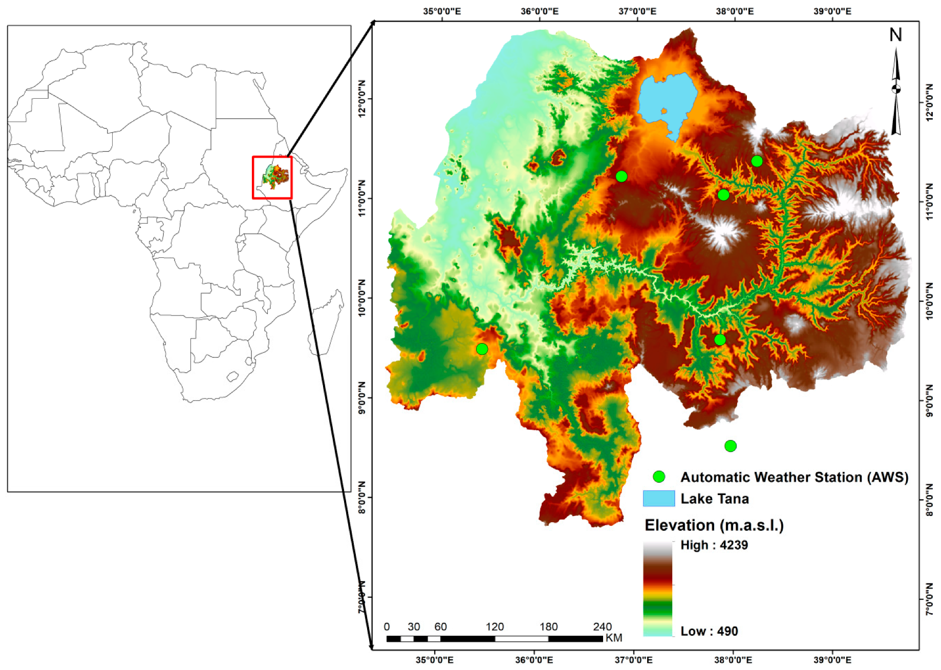
2.1. Site Description

The Upper Blue Nile (UBN) basin is located in the northwestern part of Ethiopia (Figure 1). The UBN basin is a main source of the Nile River water resource, and it contributes about 60% of the annual flow of the Nile [50,51]. The basin has an approximate drainage area of 176,000 km2 [52]. It is characterized by a complex topography with elevation ranging from 4239 m a.s.l. at the northeastern part of the basin to 490 m a.s.l. at the western part of the basin near the Ethiopian–Sudan border (Figure 1). The climate of the UBN basin ranges from humid to semi-arid. The main rainfall season (known as “Kiremt”) occurs from June to September. The dry season runs from October to January followed by a short rainy season (called “Belg”) from February to May. According to Kim et al. [53], about 70% of the annual precipitation in the study area (UBN basin) is observed during the Kiremt season. The UBN basin receives up to 2200 mm of annual rainfall. The annual mean rainfall varies between 1200 and 1800mm [52] with an increasing trend from northeast to southwest [53]. However, the basin is characterized by large temporal fluctuations in rainfall [52,54] both on intra-annual and inter-annual scale. As a result, the hydrological processes in the basin are quite complex and highly variable in space and time. Although quite a diversity of land use systems is common, the livelihoods of the majority of the populations in the basin are highly dependent on rain-fed agriculture.

2.2. Data

Remote sensing input data were acquired from Sentinel-1 SAR, Moderate Resolution Imaging Spectroradiometer (MODIS), and the Shuttle Radar Topographic Mission (SRTM). Volumetric soil moisture data were also collected from ground-based automatic weather stations (AWS) and land surface parameters simulated from the Noah 3.3 model in the Famine Early Warning Systems Network (FEWS NET) Land Data Assimilation System (FLDAS). Data were collected/acquired for the periods of 2016 and 2017 (for the months of September, October, November, December, and January). Those months, except September, are the dry periods in the study area when farmers can potentially practice additional cropping using residual soil moisture. The month of September indeed belongs to the wet period of the study area; however, the main season cropping reaches to the stage of physiological maturity and crops have limited moisture intake during this month. So, dry season farming may start as of September for efficient utilization of the residual soil moisture. Descriptions of each data are provided below.

2.2.1. Remote Sensing Data

This study used SAR image data from the Global Monitoring for Environment and Security (GMES) Sentinel-1 mission. It operates in C-Band SAR instrument with the frequency of 5.405 GHz. Sentinel-1 has four different operating modes; however, over land, it uses the main operational Interferometric Wide-Swath (IWS) mode and measured at dual polarization (i.e., vertical transmit and vertical receive—VV and vertical transmit and horizontal receive—VH) with a 250 km swath and an average temporal resolution of 12 days in the study area. Free data can be accessed via the European Space Agency (ESA) website (https://scihub.copernicus.eu/dhus/#/home) once it is acquired. In this study, 66 level-1 (for 32 acquisition dates) product of IWS mode generated as Ground Range, Multi-Look, and Detected (GRD) products were acquired for the periods of 2016 and 2017 (Appendix A Table A1, lists of Sentinel-1 SAR data used). The GRD product of high-resolution class has a spatial resolution of 20 × 5 m and a pixel spacing of 10 m. This study used data from descending orbit, which provides dual -polarized SAR data acquired both at VV and VH polarizations simultaneously. The essential characteristics of Sentinel-1 IW swath mode data are given by [55].
The preprocessing of SAR data consists of several steps including radiometric correction, speckle filtering, and geometric correction. These processes have been done using the Sentinel application platforms (SNAP) provided by ESA. The calibrations of raw SAR data have been made using the radiometric toolbox in SNAP. Radiometric calibration is required to convert SAR pixel values to exact backscattering coefficient of the scene. A 7 × 7 Enhanced Lee filtering window was applied to the SAR data to reduce the speckles that may degrade the quality of the SAR image. The geometry of the SAR data has been corrected using Range Doppler Terrain correction tool in SNAP.
Ground vegetation coverage has an effect on the backscattering characteristics of SAR data. In this aspect, the normalized difference vegetation index (NDVI) were used to assess ground vegetated land cover. For this study, MODIS NDVI data product (MOD13A2) was downloaded from the USGS earth explorer website for the period of 2016 and 2017. We have used NDVI data of MOD13A2 prepared with 16-day composite and a spatial resolution of 1 km. Daily values of MODIS NDVI were obtained by interpolating the 16-day composite using temporally corrected time-series information of composite. The digital elevation model (DEM) with a spatial resolution of 30m provided by the Shuttle Radar Topographic Mission (SRTM) was used for geometric correction of SAR data during the preprocessing phase. However, the topographic variation still determines the spatial distributions of soil moisture in the field [56] and the acquired SRTM Global elevation data was also considered in the SAR based soil moisture prediction model.

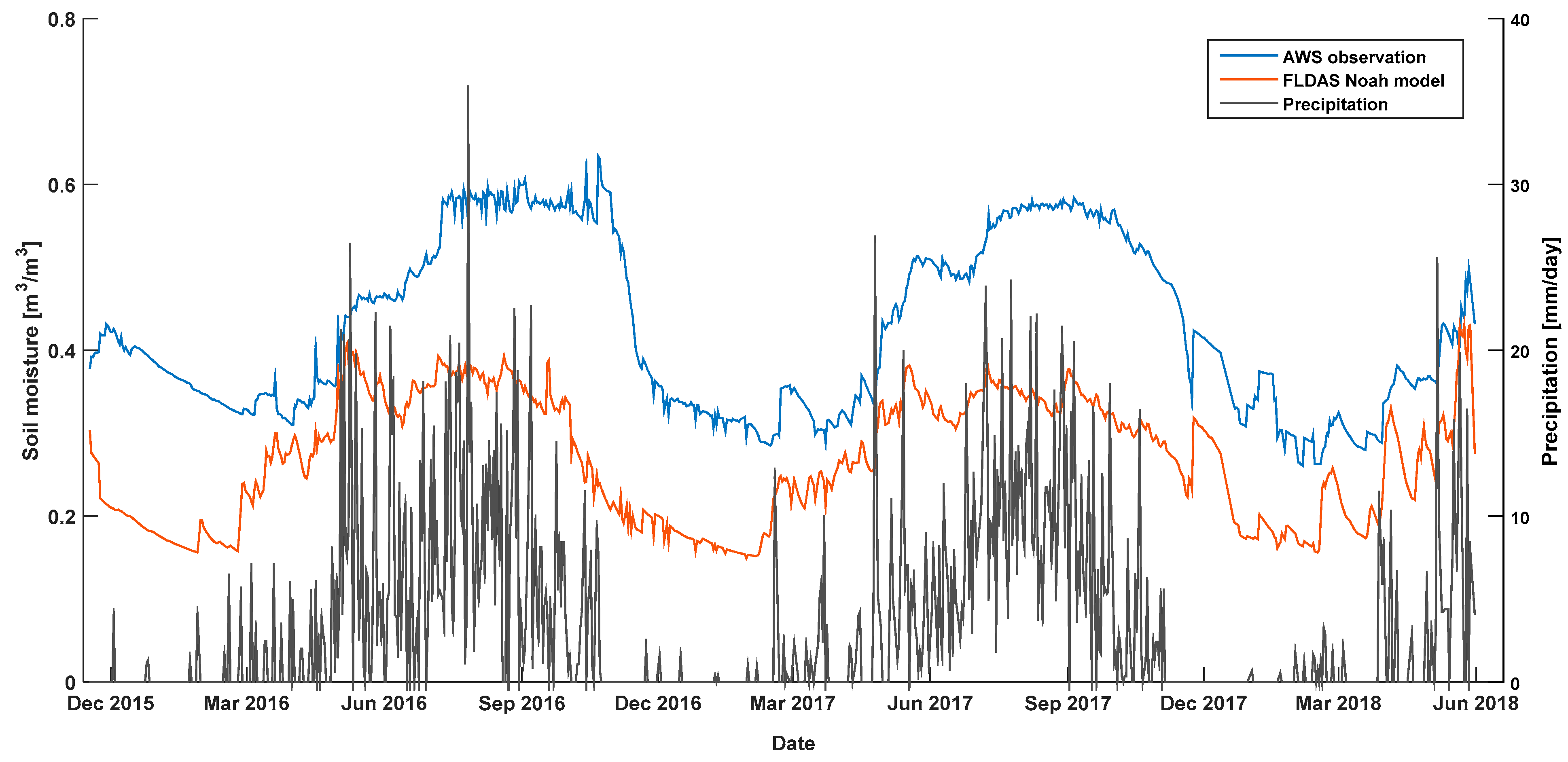
2.2.2. Soil Moisture

The prediction models in this study were calibrated and validated using known volumetric soil moisture data obtained from automatic weather stations (AWS) and FLDAS Noah model simulated for East Africa.

Ground Observed Soil Moisture Data

Ground observed soil moisture dataset is valuable for model calibration and validation when we are dealing with soil moisture estimation using remote sensing data. However, many African countries, including Ethiopia, are characterized by the scarcity or unavailability of ground based soil moisture observations [57]. Recently, the National Meteorological Agency (NMA) of Ethiopia has installed about 16 automatic weather stations (AWS), which can measure soil moisture data at different depths of soil in addition to other climatic information.
For this study, only six stations are found in and around the UBN basin, corresponding to the acquisition of Sentinel-1, were used for the period of 2016 and 2017. The six stations are “Dangila”, “Kachis”, “Motta”, “Nedjo”, “Simada”, and “Weliso” (Figure 1). At each site, soil moisture measurements are taken at 20, 50, and 100 cm depth with a 15 minutes time interval. To overcome the absence of calibration standards, the spatiotemporal distributions of AWS (0 to 20 cm) data sets have been compared to FLDAS Noah soil moisture product (0 to 10 cm depth) and Climate Hazards Group Infrared Precipitations with Stations (CHIRPS) satellite rainfall product. The CHIRPS has shown good agreement with ground observed rainfall over our area of interest [58]. To define the spatial patterns in the relationship, a point to pixel-wise correlation between the daily mean of all the six AWS observed volumetric soil moistures with that of FLDAS Noah and CHIRPS precipitation has been made (Figure 2). Within this domain, AWS observations have shown consistent spatiotemporal distribution with the simulated FLDAS Noah and CHIRPS precipitation events (Figure 2). A strong correlation of AWS measured volumetric soil moisture with simulated FLDAS Noah (r = 0.74) and CHIRPS precipitation (r = 0.53) can be noted.
It is also noticed that the inconsistency of the soil depth measured by AWS (0 to 20 cm) and the sensitivity of C-band SAR data are usually more responsive to the top few centimeters of soil [59]. However, [60] have observed that the sensitivity of the C-band SAR data to soil moisture variation could extend up to 20 cm depth. For example, Humphrey [61] has found a significant correlation between backscatter variables extracted from the C-band RADARSAT imagery and soil moisture measured at both 5 cm and 20 cm depths, with r = 0.83 and 0.79, respectively. Similarly, [62] reported the sensitivity of RADARSAT-2 SAR data to the amount of soil moisture measured at 20 cm depth and resulted in a correlation value of 0.85. A correlation value up to 0.84 between backscatter values from ERS SAR data and in-situ soil moisture also observed at a depth of 20 cm [63]. Therefore, these may suggest the sensitivity of C-band SAR data up to 20 cm depth measurements of soil moisture and could be used to calibrate a soil moisture prediction model using Sentinel-1 SAR data. However, still readers should note that the vertical heterogeneity of soil moisture at 20 cm depth of soil could affect the relationship between SAR backscattering and volumetric soil moisture and might affect model prediction performance. It is also clear that a better correlation and model inversion performance would be observed with soil moisture measured at a top few centimeters of soil.

FLDAS Noah Model

To expand the spatial and temporal evaluation of the proposed method (SCA), a model-based soil moisture product has been used as an additional resource. Thus, FLDAS Noah model (simulated for East Africa) was used in this study, in addition to ground AWS, to calibrate and validate the SCA method [64]. The FLDAS Noah model is simulated from the widely used Noah land surface model and provides volumetric soil moisture data at different soil layers and spatiotemporal resolutions [64]. In this study, the top 10 cm soil layer moisture content with a spatial resolution of 0.1 × 0.1 degree was obtained from the NASA Goddard Earth Science Data and Information Services Center (GES DISC) web site. The FLDAS Noah measurements that correspond to Sentinel-1 SAR temporal coverage are available for 2016 and 2017 at a daily time step.

2.3. Methods

Volumetric soil moisture from both AWS observations and FLDAS Noah model were used as a dependent variable, while backscatter values of both VV and VH polarizations from Sentinel-1 SAR, vegetation information based on NDVI analysis, and elevation information derived from DEM data were considered as independent variables to calibrate and validate the model. The Sentinel-1 SAR data and DEM were provided with a spatial resolution of 10 and 30 m, respectively. Therefore, for the first model based on AWS observation, average values of backscatter measurements and elevation within a 1 × 1 km ground area were used to keep the spatial resolution consistent with MODIS NDVI. In this case, it was assumed that point measurement at the ground station is representing the average soil moisture in the area corresponding to remote sensing data. The main limitation is still the necessity for having sufficient number of distributed ground observation at each satellite footprints/grid cells in order to assure that the assumption of point measurement is corresponding to satellite observations. Similar methods of data preparation were applied to soil moisture data obtained from the FLDAS Noah model. Dual-polarized Sentinel-1 SAR, NDVI and DEM data measurements were resampled to the ground resolution of ~ 10 × 10 km in order to match with the spatial resolution of FLDAS Noah soil moisture.
Studies have reported that soil moisture radar backscattering is affected by a number of time and space varying parameters such as vegetation, soil property, and topography [14,65,66]. Thus, our study was started by investigating the effect of each remote sensing input variable for soil moisture estimation in our area of interest. So, the linear regression analyses between remote sensing data and volumetric soil moisture was conducted (Table 1). The simple linear regression was first done between backscattering values from VV polarization and volumetric soil moisture and then the multiple regressions were continued using VV and VH radar backscattering values. Afterward, in a step fashion, the other independent variables (i.e., vegetation and elevations) were sequentially added to the regression model.
The models’ coefficient of correlation (r) values were used to evaluate the soil moisture prediction performance of each model. All the regressions in Table 1 have a significant correlation at p < 0.01 with volumetric soil moisture (for both AWS observed and FLDAS Noah simulated model). The combination of VV and VH polarization has shown a slight improvement in the correlation values but VH backscatter seems to be important for the overall performance of the model. The inclusion of vegetation (NDVI) into the regression model has considerably improved the correlation values to 0.63 and 0.57 for AWS and model simulated soil moisture, respectively. The effect of elevation cannot be ignored in our case and its inclusion in the modeling process has further improved the prediction performance of the model with r 0.76 (0.65) for AWS (model simulated) soil moisture. Thus, to get complementary information from all these remote sensing variables, it was decided to feed a combination of σ V V , σ V H , NDVI, and E as input parameters to the proposed stepwise-cluster analysis model. According to [67], the combined use of remote sensing data obtained from different sensing systems (e.g., microwave and optical sensing system), can grant complementary information regarding the extent of soil moisture content in a given land use class.

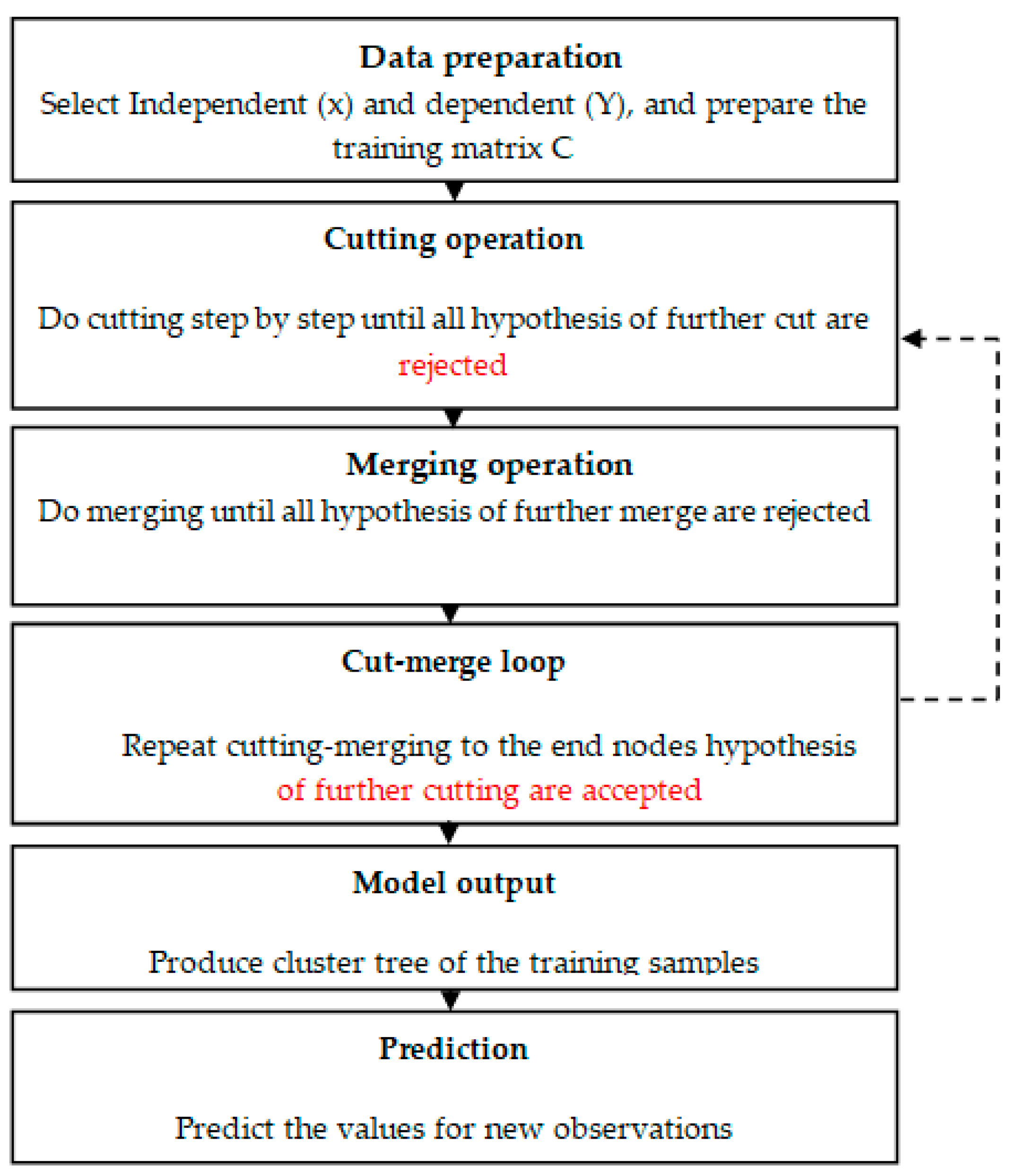
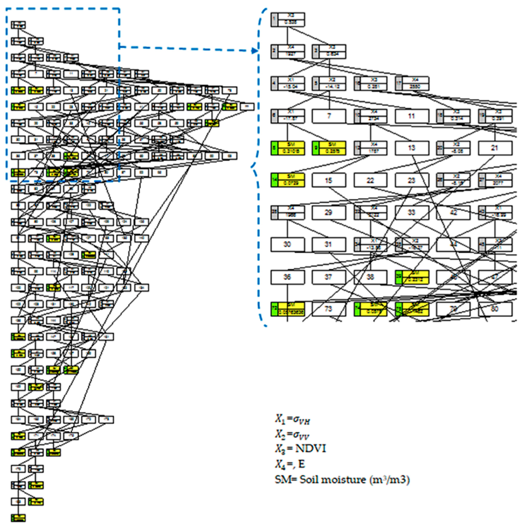
2.3.1. A Stepwise Cluster Analysis (SCA)

Model Development

Considering the complexity and non-linearity of retrieval problems, a statistical relationship between volumetric soil moisture and remote sensing variables (i.e., σ V V , σ V H , NDVI, and DEM) was established using a SCA model. The principle of SCA is to divide samples (containing a number of independent and dependent variables) into a set of clusters with significant differences based on a series of cutting (i.e., splitting one set into two) and merging (i.e., joining two sets together) process according to a given statistical criterion [40,41,42]. Similar to other nonparametric tree regression statistical methods such as the Random Forest (RF), SCA can effectively capture the inherent nonlinear relationship between predictors and predictands [68], apply a defined set of criteria to split and merge datasets into different nodes, and use the regression tree method for predicting. However, unlike the SCA method, the RF uses a bootstrapping method for training/testing the model [69]. While splitting the tree’s node, RF searches for the best features, among a random subset of features instead of searching for the most important features from the dataset. In addition, RF uses multiple decision trees for prediction, afterward these decision trees are merged together to get more stable estimation [70].
Basically, the SCA approach follows four major steps: (i) set criteria for cutting and merging clusters-, based on Wilks statistic [71], (ii) cutting/merging clusters operation-based on the criteria, (iii) produce single SCA cluster tree-, that contains a set of prediction nodes, and (iv) prediction. Generally, the SCA clustering process begins with a cutting action by which the original training sample dataset will be split into two groups. Then, the merging and cutting loops will be continued up until none of the sub-clusters can be further divided or merged with other sub-clusters. Finally, a cluster tree which contains a set of prediction nodes (tip cluster) will be generated from the training sample datasets and used to predict the dependent variable for any new values of the independent datasets. The flow of SCA model development is given in Figure 3.

Training

In order to train the SCA model, first, the original datasets were divided into training and testing datasets randomly. The training sample datasets contains a set of independent ( σ V V , σ V H , NDVI, and DEM) and dependent variables (volumetric soil moisture). Assuming that there are n α samples, with m independent variables (X) and one dependent variable (Y). Thus, the training set can be given as one cluster ( C ), shown as the following equation (Equation (1)):
C = [ X 1 , X 2 , , X m , Y ] = [ x 11 , x 12 , , x 1 m x 21 , x 22 , , x 2 m y 1 y 2 x n C 1 , x n C 2 , , x n C m y n C ]
Thus, a cluster tree can be derived through cutting and merging operation of the training set following the cut-merge loop provided in Figure 3.
Let cluster C , which contains n C samples, be cut into two sub-clusters β and γ , which contain n β and n γ samples, respectively ( n C = n β + n γ ) . According to Wilks’ likelihood-ratio principle, the cutting point is optimal only if the value of Wilks statistic Λ is minimum [40,71]. The smaller the Λ value refers the larger the difference between the sample means of β and γ sub-clusters. When the Λ value is very large, sub-cluster β and γ cannot be cut and must be merged instead. According to Rao’s F-approximation [61], the Wilks Λ statistic under the above two sub-clusters ( β and γ ) can be correlated to F-variant as follows (Equation (2)):
F = ( P , n β + n γ P 1 ) = 1 Λ Λ n β + n γ P 1 P
where P = number of predictors. Since the Λ is related to the F statistics, the sample means of the sub-cluster β and γ can be evaluated for their significant differences using an F-test [39]. Therefore, cutting (or merging) of clusters will be decided based on the F tests [72]. The null hypothesis would be H 0 : μ β = μ γ versus the alternative hypothesis H 1 : μ β μ γ , where μ β and μ γ are sample mean of β and γ . Let the significance level be α . In this study, the sensitivity of modeling result has been tested for different significance levels (i.e., α = 0.01 , α = 0.05 , and α = 0.1 ). An operation of cutting would be applied if: F c a l F α and H 0 is false, which implies that differences of means between two sub-clusters are significant; whereas, F c a l < F α and H 0 is true would be the merging action that indicates these two sub-clusters have no significant variations.
All the sub-cluster produced from the original training sample dataset will go through a number of iterative runs of cutting and merging processes and the training procedures are completed when all tests are undertaken and all hypotheses of further cut (or merge) are rejected. Then, a cluster tree can be obtained. Afterward, Y can be predicted for any new input data of X using the derived cluster tree. A cluster tree usually contains a tip cluster and a series of cutting and merging rules. Tip clusters are those clusters that contain the prediction systems, which can no longer be split or merged with others. Usually, the mean value of the tip cluster is used to estimate the predicted results [41].

Prediction

Following the completion of model training, a cluster tree can be derived for a new sample prediction. The prediction is indeed a searching procedure by itself, starting from the top of the tree and ending at a tip cluster, following the route lead by the cutting and merging rules [45]. When a new sample ( x 1 , x 2 , , x m , y p : y p   i s   u n k o w n ) enters the tree at a cutting point, step-by-step the sample set will eventually drop into one of the tip sub-cluster which cannot be either cut or merged further. The right tip sub-cluster is determined by the routes (or values) of new independent variables ( x 1 , x 2 , , x m ). The predicted value of y p will be the mean of dependent variables of the training samples in that tip cluster. Let cluster e be the tip cluster where the new sample { x m } enters. The predictand { y p } is (Equation (3)):
y p = y p e ± R p e
where y p e = mean of dependent variable (e.g., volumetric soil moisture) in sub-cluster e (Equation (4)) and R p e = radius of y p in sub-cluster e (Equation (5)).
y p e = 1 n e k = 1 n e y p , k e ,
R p e = { m a x [ y p , k e ] m i n [ y p , k e ] } / 2 ,
The correlation coefficient (r) and the root mean square error (RMSE) were used to evaluate the performance of the SCA model during the training and testing periods. The software packages (called rSCA) included in ‘R’ statistical packages were used in this study [73]. To examine the performance of the developed model, SCA was compared with a nonlinear support vector regression (SVR) method.

2.3.2. Support Vector Regression (SVR)

The support vector regression (SVR) technique is based on the structured risk minimization principle. This method maps the input data into a high dimensional feature space using non-linear mapping and then a linear regression problem is obtained in the feature space. A set of training data ( x i , y i ) is considered where x i is the input vector (e.g., the SAR backscattering coefficients) and y i is the corresponding output vector (e.g., the volumetric soil moisture); i = 1, 2…, L and L is the total number of data pairs, y R, x RD. The aim of the SVR model is to find a function f ( x ) that has at most ε -deviation from the actually obtained targets for all the training data (Equation (6)). The function is given as [74]:
f ( x ) = w , x + b
where w , x denotes the dot product of a weighted vector w and input vector x, and b is the bias. The first prediction is attained according to ε -insensitive losses function, where ε quantifies the tolerance to errors. A penalty function is applied to the output variables if the predicted value is greater than a distance ε from the actual values and, the penalty can be represented by one of two slack variables ξ i and ξ i * (where ξ i 0 , ξ i * 0 i ) (Equation (7)). The cost function to minimize can then be written as:
1 2 w 2 + C i = 1 L ( ξ i + ξ i * )
Satisfying the following constraints (Equation (8))
{ y i [ w . x i + b ] ε + ξ i , [ w . x i + b ] y i ε + ξ i * , i = 1 , 2 , L ξ i , ξ i * 0 ,
where C is a regularization parameter determining the tradeoff between the training errors and the complexity of the function f ( x ) . The slack variables decide the degree to which sample data points are penalized if the error is greater than ε . Therefore, for any (absolute) error small than ε , ξ i = ξ i * = 0. The constrained optimization problem in Equation (7) can be solved using dual formulation. In dual formulation, Lagrange multipliers α   and   α * , are used and the minimization problem is solved by differentiating relating to the primary variables (Equation (9)). The final estimation function can then be written as follows:
f ( x ) = i = 1 N ( α i α i * ) k ( x , x i ) + b ,
where α   and   α * are Lagrange multipliers; and k ( x , x i ) is the kernel function. A kernel function measures non-linear dependence between the two input variables x   and   x i . The x i ’s are “support vectors” and N (usually N L) is the number of selected data points or support vectors corresponding to values of the independent variable that are at least ε away from actual observations.
Several nonlinear kernel functions such as Radial Basis Function (RBF), linear, polynomial, and sigmoid have been proposed [75]. The RBF kernel (Equation (10)) performs better in comparison to other kernel functions [76]. The nonlinear radial basis function is defined as:
k ( x , x i ) = e x p ( x x i 2 2 σ 2 )
where σ is known as the kernel parameter (radial width).
Thus, a nonlinear SVR model using RBF kernel was developed to estimate residual soil moisture. The SVR model was tuned and the optimum values for insensitive loss function ( ε ) , regularization parameter (C), and kernel parameter ( σ ) were used. In this study, an internal 10–fold cross-validation during the development of SVR model was used for the optimal combinations of the three parameters.

3. Results

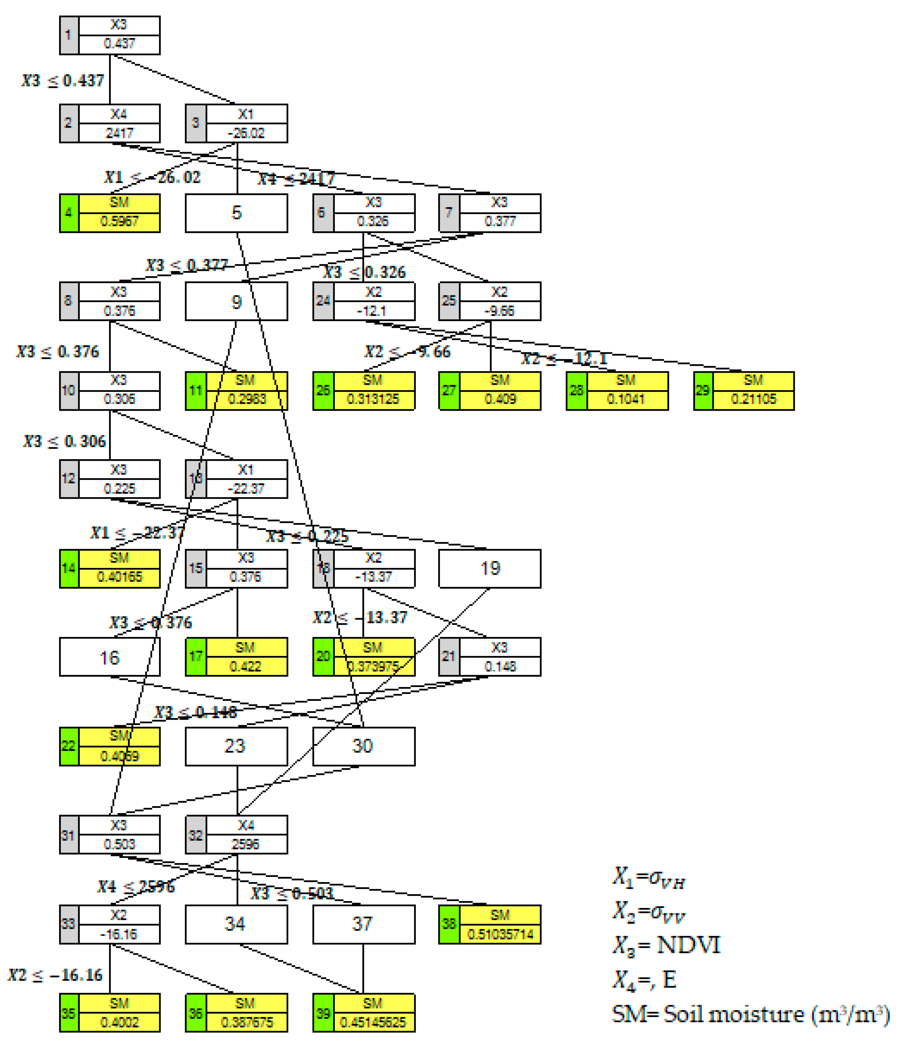
3.1. Stepwise Cluster Analysis

In this study, two different SCA cluster trees were generated to show the relationship between remote sensing variables and volumetric residual soil moisture (obtained from both AWS observations and model simulations). The prediction performance and the structure of the SCA tree could be affected by the internal parameters such as the cutting (or merging) action of clusters governed by the significance level ( α ) used in the analysis. According to Sun et al. [41] and Wang et al. [45], SCA analysis at different significance level could lead to different cluster trees with a different number of cluster nodes and predictions. Thus, it is vital to iteratively run SCA model adjusting for different significance levels until the prediction model showed the finest performance in reproducing observed values. The SCA cluster model, in this study, has been verified for different significance levels (i.e., α = 0.01 , α = 0.05 , and α = 0.1 ). Table 2 provides the statistical performance of the SCA cluster tree at different significance levels during training and testing phases. Also, Figure 4 provides the scattering properties of predicted values obtained from different significance levels during the testing periods.
Results in Table 2 indicated that the number of cluster nodes and cutting operations is increased with an increase of α from 0.01 to 0.1. The SCA cutting (or merging) action, as well as the rejection of the iteration process, relied on this parameter. Model with α = 0.1 produced a more complex cluster tree among the three significance levels and produced a large number of cluster nodes, due to more cutting actions than the others (Table 2). The reason for this is that the higher α value results in the decreased strictness in the cutting operation [41,45]. Thus, the higher α value will lead to more cutting actions and more cluster nodes. According to the statistical results in Table 2, different values of significance levels lead to distinct prediction results. However, a good agreement was found between remote sensing based estimates and observed/simulated volumetric soil moisture for all significance levels of the SCA model.
For AWS based SCA model (Table 2), there is a slight improvement in predicting volumetric soil moisture while α value increases from 0.01 to 0.05, with r being 0.95 (0.87) and RMSE 0.032 (0.097) m3/m3 during training (testing) phase. Although further increasing α value to 0.1 leads to the higher number of cluster nodes and cutting actions, it resulted to decrease the statistical performance of the prediction model, except a slight improvement in RMSE (0.088 m3/m3) during the testing phase. Thus, the AWS based SCA model with α = 0.05 is an optimal model for predicting volumetric residual soil moisture in our area of interest.
In the case of FLDAS Noah SCA model, an optimal prediction performance was observed when the α value was set to 0.01 with r being 0.93 (0.87) and RMSE 0.043 (0.058) m3/m3 during the training (testing) phase. In fact, the performance of the prediction model has improved while the α value increases from 0.01 to 0.1 for the training datasets but not confirmed during the testing period. Thus, the validation result clearly demonstrated that the SCA model is a reliable technique for soil moisture prediction using remote sensing data.
Also, Figure 4 shows that at a lower significance level (i.e., α = 0.01 , in Figure 4a,d) the prediction models have produced several redundant values, but still with strong correlation coefficients, for a single value of AWS observed and FLDAS Noah volumetric soil moisture. Thus, plots in Figure 4a,d have presented intense horizontal lines. However, as the significance level increased (Figure 4b,c,e,f), the prediction models have produced a relatively wide range of values. The two optimal SCA prediction model derived from the combinations of SAR and optical remote sensing data (Figure 4b,d) have shown a good performance in predicting maximum and minimum soil moisture values observed/simulated by automatic weather stations and FLDAS Noah model. The SCA has managed to produce volumetric soil moisture with an overall bias value of 1.21 and 0.99, where a value of 1 is a perfect score, in comparison to AWS observed and FLDAS Noah simulated soil moisture, respectively. Thus, the overall agreement between observed/simulated and predicted soil moisture indicates that coupling of satellite data (e.g., Sentinel-1 SAR and NDVI) and the nonlinear SCA approach is capable of detecting surface soil moisture and its spatiotemporal dynamics.
Figure 5 and Figure 6 gives the two optimal SCA cluster trees for the case of AWS and model simulated soil moisture. The cluster tree clearly shows the role of every independent remote sensing parameter in describing the relationship. Both Figure 5 and Figure 6 demonstrated that X 3 (vegetation) is the most important variable that determines the accuracy of residual soil moisture prediction of the model. The other independent variables ( X 1 = backscattering from VH polarization, X 2 = backscattering from VV polarization, and X 4 = elevation information) also have a profound effect on the predicted volumetric soil moisture. Based on these trees, the residual soil moisture values for new observations of the remote sensing variables can be predicted.
For example, let X 1 = −20.4, X 2 = −4.5, X 3 = 0.41 and X 4 = 2100 as a new observations for Figure 5 (AWS model) cluster tree. To predict the residual soil moisture: the new values: X 3 0.437 for the first cluster so that the sample input enters to cluster 2; X 4 2017, so that it enters to cluster 6; X 3 > 0.326, so that it enters to cluster 25; X 2 > −9.66 so that it finally enters to tip cluster 27 with a soil moisture prediction value of 0.409 m3/m3. On the same cluster tree (Figure 5), let us take another input sample, X 1 = −20.4, X 2 = −22.5, X 3 = 0.35, and X 4 = 2500. Then to predict the volumetric residual soil moisture for these new input variables, for the first branch X 3 0.47, so that it enters to cluster 2; X 4 > 2417 so that it enters to cluster 7; X 3 0.377, so that it enters to cluster 8; X 3 0.376, so that it enters to cluster 10; X 3 > 0.306, so that it enters to cluster 13; X 1 > −22.37, so that it enters to cluster 15; X 3 0.376, so that it enters to intermediate cluster 16 and 30 and then merged to cluster 31; X 3 0.503, so that it enters to intermediate cluster 37 and then finally enters to cluster 39 with a prediction value of 0.45 m3/m3. Similarly, it is possible to find the prediction values for new observations using FLADAS Noah cluster tree (Figure 6).

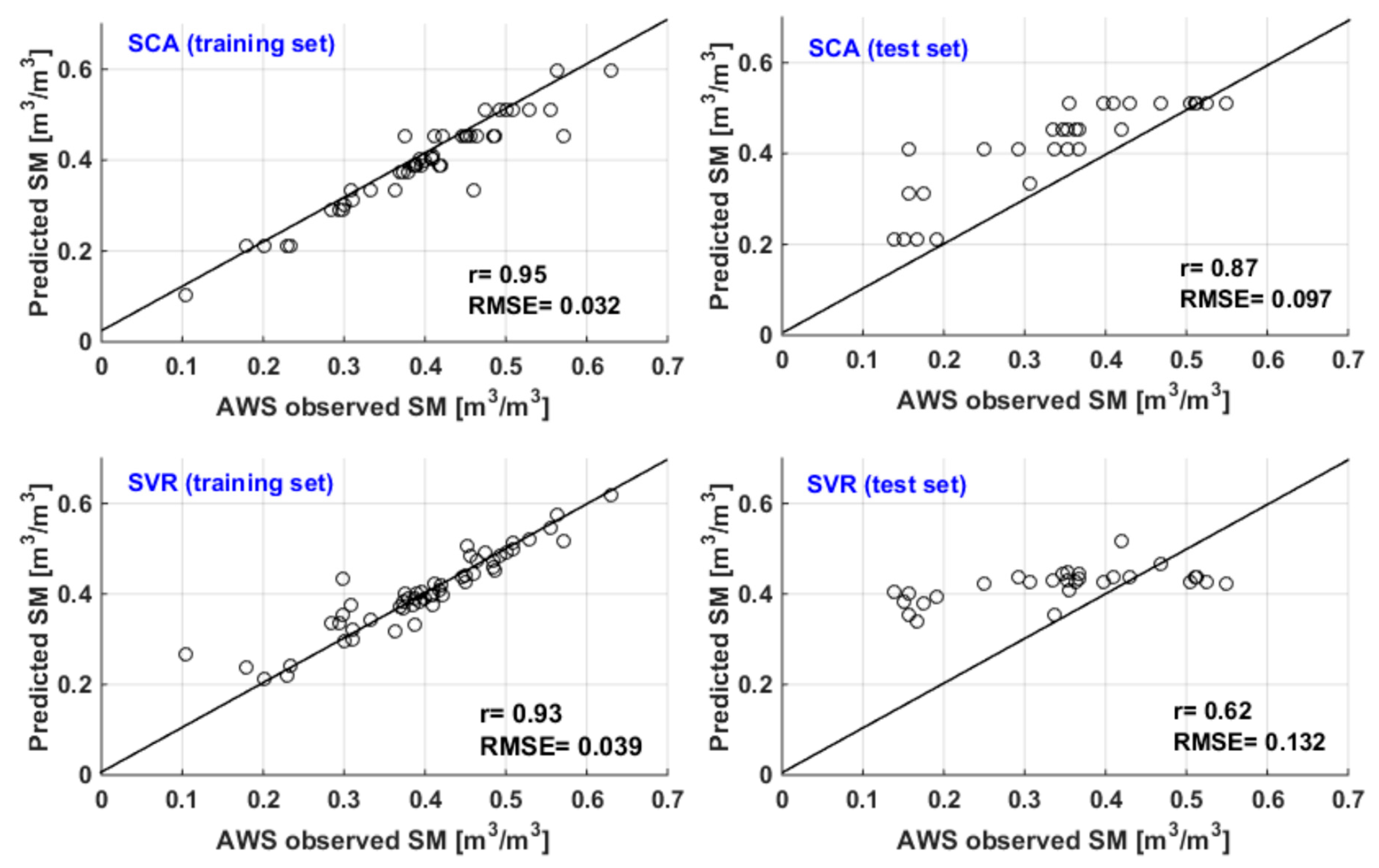
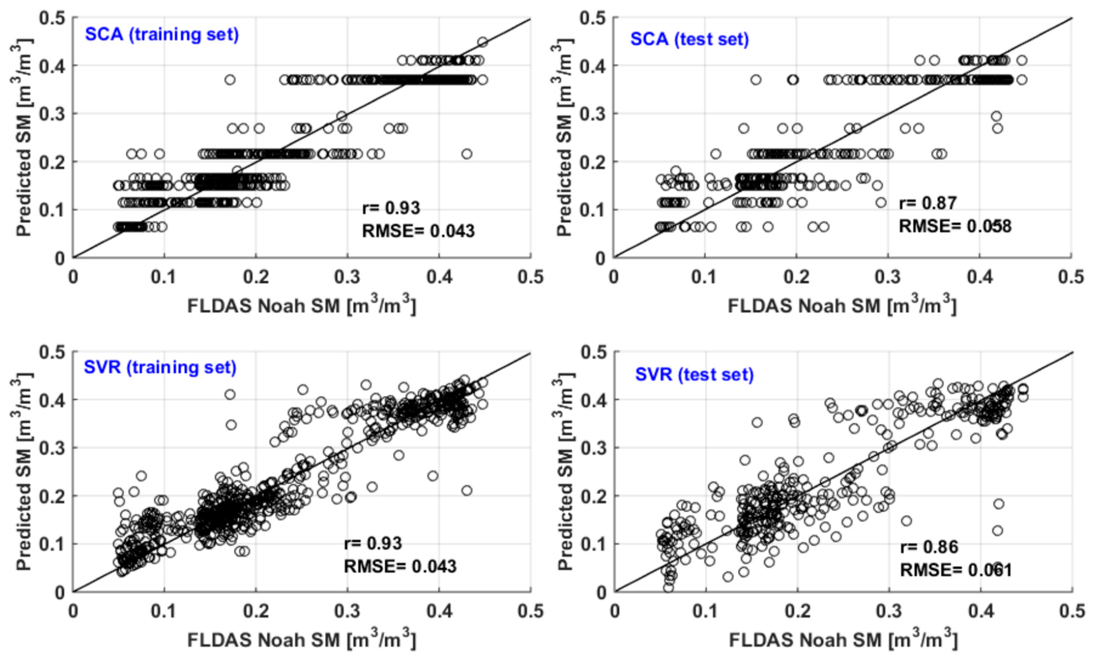
3.2. Comparing SCA with SVR Method

Results of the SCA model were also compared with the SVR, state-of-the-art techniques used for soil moisture prediction using remote sensing data [36,38]. The SVR model, using the same datasets as those used for the two clusters, was developed. Then, quantitative evaluation between model predicted and observed/simulated soil moisture were implemented (Figure 7 and Figure 8). Scatter plots in Figure 7 presents the comparison between the model (SCA and SVR) predicted and AWS observed residual soil moisture both during the training and testing periods. In this case, both SCA and SVR model have shown a comparable performance in predicting residual soil moisture. However, the proposed method (SCA) outperformed the SVR model for predicting residual soil moisture in our area of interest (Figure 7) in terms of Pearson correlation coefficient (r) and the root mean square error (RMSE).
The statistical parameter during the training phase showed SCA’s highest r = 0.95 and lowest RMSE = 0.032 m3/m3, in comparison to, SVR model’s r = 0.93 and RMSE = 0.039 m3/m3. The superiority of SCA over SVR prediction model was clearly demonstrated during the testing phase with r = 0.87 and RMSE = 0.097 m3/m3, in comparison to, SVR’s r = 0.62 and RMSE = 0.132 m3/m3.
Also, Figure 8 gives the comparison made between the model predicted and the FLDAS Noah model simulated soil moisture both during the training and testing phase of the analysis. The SCA soil moisture model has shown as good a performance as the SVR method, with slightly better prediction accuracy during the testing phase. The SCA model achieved r = 0.93 (0.87) and RMSE = 0.043 (0.058) m3/m3, while SVR method resulted in r = 0.93 (0.86) and RMSE = 0.043 (0.061) m3/m3 during the training (testing) phase. In general, the result implied the better fitting and predictive performance of SCA tree relative to the SVR when dealing with the nonlinear relationship between remote sensing variables and volumetric soil moisture. In addition, unlike SVR, SCA produced a cluster tree that shows the links among variables and one can clearly identify the role of every independent variable in mapping the relationships.

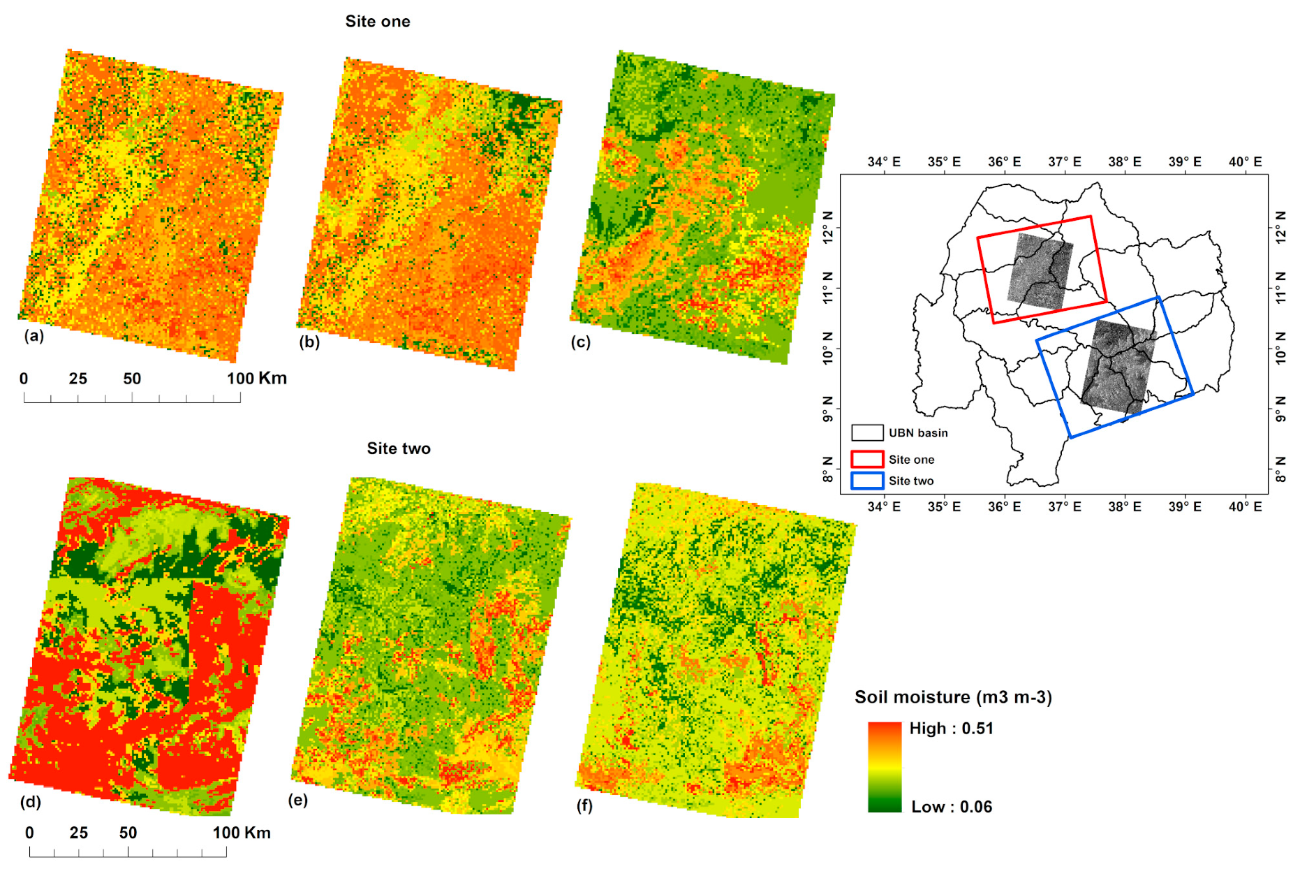
3.3. Spatial Patterns of Estimated Soil Moisture

Six soil moisture maps, for two selected sites of the study area, were presented from the time series to demonstrate the spatial variability of estimated soil moisture (using AWS based SCA prediction model) at various dates (Figure 9). The spatial patterns of soil moisture in both sites (site one and site two) follow the meteorological and geomorphological conditions of the selected area. The higher soil moisture values for both sites have been observed in areas relatively with high vegetation cover and elevation values. Most parts of the sites with scattered vegetation and lower elevation have shown a comparatively small amount of estimated soil moisture values.
Thus, the higher soil moisture values for the site are observed in the southeastern and northwest parts, which appear towards the highest elevation and vegetation coverage areas. While the lower estimates are observed in north and south ends of the site that can be characterized by a relatively low elevation and scattered vegetation condition. With the same spatial pattern in site two, the higher soil moisture values are observed in higher elevation and vegetation areas situated in the south and southeastern parts, while their lower values are concentrated in the north and central parts. Indeed, for the selected dates in site one and site two the estimated soil moisture values are reasonably high in most places on 28 September 2016 (Figure 9a) and 29 October 2016 (Figure 9d), respectively, due to rainfall events and good surface moisture conditions on these dates. However, the spatial distributions of soil moisture are gradually reduced in the other dates (e.g., 22 October 2016 and 22 November 2016) following the dry days, with the exception of the river catchment areas, which are described by higher values of soil moisture even during the dry periods.

4. Discussion

Previous studies (e.g., [16,17,18,19,20,21,22,77,78,79]) demonstrated that surface soil moisture (representing 0–5 cm depths) can be derived from SAR data. However, the radar backscattered signal is not only dependent on the soil moisture content but also sensitive to other time and space varying parameters such as vegetation, topography, and soil properties [14,65,66]. Thus, the linear relationship, between volumetric soil moisture and sentinel-1 SAR backscatter coefficients, made in this study result in lower r (0.34 to 0.36) values. Indeed, the lower r values in our study might not only attributed to the effect these surface parameters but it could be also due to the reduced sensitivity of SAR to soil moisture observed beyond the top few centimeters of soil. Note that simulated and observed soil moisture datasets at 10/20 cm depth of soil were used in this study. However, incorporating additional ancillary variables such as vegetation and elevation conditions of the study area have improved the linear models with r (0.65 to 0.76). Moreover, scholars (e.g., [36,56]) argued that incorporating these and other ancillary variables have further increased the accuracy of SAR based soil moisture prediction using the nonlinear regression model, such as SVR and artificial neural network (ANN) techniques. Although using more predictors would lead to more computational complexities, it can help to develop a more comprehensive relationship and further improve the model prediction performance [47].
In this paper, SCA was used as an alternative statistical approach intended for modeling the nonlinear relationships between remote sensing variables (i.e., dual-polarized Sentinel- SAR data, NDVI, and DEM) and volumetric soil moisture. The SCA model has been trained for volumetric soil moisture obtained from both AWS and FLDAS Noah models.
Previous studies (e.g., [45,46,47,48,49]) applied SCA method in different disciplines have shown that SCA model is characterized by higher performance in describing the nonlinear relationship between state variables and dependent variables and better accuracy in predicting observed values. Our findings support these observations using the relationship between volumetric soil moisture and remote sensing data. The SCA generated cluster trees could be used to predict volumetric soil moisture given inputs of the remote sensing variables. However, the process of SCA analysis is affected by a number of internal parameters such as the significance level [41,45]. Accordingly, various significance levels (i.e., 0.01, 0.05 and 0.1) have resulted in different cluster trees so that a considerable effect on the prediction performance of SCA model has been observed. Thus, an optimal soil moisture prediction cluster tree for AWS and FLDAS Noah based analysis was obtained at α = 0.05 and α = 0.01, respectively. Our result is consistent with the findings of [41], who applied the SCA model for microbial biomass prediction in food waste compositing, with an optimal prediction performance of α = 0.05 and α = 0.01 for thermophilic and mesophilic bacteria, respectively. This implies that an optimum prediction level of the SCA model could be affected by the type and the scale of datasets used in the calibration. Thus, for every dataset an iterative run that is adjusted for different significance levels is the best approach to obtain optimal prediction models using the SCA method. However, at lower significance levels our prediction models have produced several redundant values (still with strong correlation coefficients) for a single value of observed and simulated soil moisture. The same result has been obtained by [41,49] using the SCA method for the prediction of microbial biomass and concentrations of pollutants at lower significance levels, respectively. This could possibly be due to the limited cutting actions at lower significance levels, which in turn results in a lower number of tip clusters (prediction nodes).
The SCA method could not only help to provide the nonlinear relationships between remote sensing parameters and soil moisture, but also provide a cluster tree that shows the links among remote sensing variables and the effects of each variable on residual soil moisture values [49]. This could give us the basis for further understanding the inherent mechanism and determining critical characters of the soil moisture prediction model [47]. The beauty of SCA lays on its step-wise-regression method in which it iterative selects the most important covariates in the prediction model. Thus, each prediction node (tip clusters) contains the most important covariate variables according to the given statistical criteria, instead of incorporating all possible variables in the model. This could contribute in reducing/controlling the overfitting problem often shown in statistical prediction models [80]. Thus, our prediction tree (Figure 5 and Figure 6) indicated that NDVI is the most important input variable, incorporated in each tip clusters, which has a significant effect on the output of the SCA model in comparison to SAR backscattering values and elevation information. Thus, the prediction accuracy of our model is highly controlled by the vegetation conditions of the study area. However, the SAR backscattering and DEM input variables have also a profound effect on the model and important for the optimum results. In this regard, our findings demonstrated the importance of integrating Sentinel-1 SAR data with ancillary surface variables obtained from other optical and/or microwave satellites for the finest prediction of surface soil moisture.
The support vector regression (SVR) method was analyzed to further illustrate the performance of SCA in soil moisture prediction, and the results are presented in Figure 7 and Figure 8. The SCA method performs well in predicting residual soil moisture, particularly during the testing periods, with smaller prediction errors and higher correlation coefficients than the SVR model. Previous studies that applied the SCA model for predicting stream flow, hydrological process, and urban air quality have also confirmed the better fitting and predictive ability of SCA relative to other statistical methods such as random forest, ANN, and SVR [46,47,48,49]. The relatively good prediction accuracy by SCA method might be related to SCA’s ability to discriminate the most important predictors and apply cutting/merging actions through searching for the minimum Wilks’ statistics (Λ) in each step of the process [56]. Simply put, in the SCA, the optimal cutting point, which split the original sample dataset into two sub-clusters is determined through sequencing the values of the predictor ( x m ). When the samples are sequenced according to the values of x m , should satisfy that Λ is minimum comparing to that of any other cutting alternatives using other predictor variables in the model. Then, the SCA analysis will calculate the mean of each sub-cluster and test for their mean difference using an F-test. If a significant difference between the two sub-clusters is observed, we can confirm that the original sample cluster can be cut into two sub-clusters using the optimal cutting point. Then, x m is identified as the most important predictor, which considerably affects the values of the predictands. If the mean difference of the sub-cluster is insignificant, the sample cluster cannot be cut and the analyst will go for testing other alternatives until no cluster can be further cut. Therefore, our finding indicates the potential of the SCA method and it could be used as an alternative statistical approach for soil moisture prediction using remote sensing data.
Our models (including SVR method) prediction error seems to be high in comparison to previous SAR/remote sensing based soil moisture prediction studies (e.g., [23,24,25,36,37,38]) and showed an overestimation of soil moisture in comparison to AWS observed values. This could be attributed to (i) the limited number of ground observed stations-with the limited number of observation stations, it is difficult to entirely characterize the spatial patterns of soil moisture over the study area, (ii) the use of soil moisture observed/simulated at 20/10 cm soil depth during model development, while microwave signals at the C-band are more sensitive to volumetric moisture to the top few centimeters of soil [81], (iii) spatial scale difference between ground observed points and satellite footprints/pixels, and (iv) sub-pixel heterogeneity of land surface conditions for lower scale analysis. Also, the overestimation of the model could be explained by the reduced relationship that could be established by low SAR backscattering values and volumetric soil moisture observed at 20 cm depths of soil during the dry periods. Because, being the dry season of our study period, where there is no/small amount of rainfall events and evaporation, leads to high vertical heterogeneity of soil moisture (i.e., sharply reduce the relationship between surface and 20 cm depth moisture) and low amounts of surface moisture, which in turn results in low backscattering values. The model reliability in this aspect could be improved further using a large number of distributed soil moisture datasets measured at a 5 cm depth of soil.

5. Conclusions

The aim of this paper was to develop a stepwise-cluster soil moisture inference model by analyzing the nonlinear relationships between multisource/multi-temporal remote sensing data and volumetric soil moisture in the Upper Blue Nile basin. Sentinel-1 SAR data, MODIS, and SRTM have been used as a source for dual-polarized SAR data, NDVI and elevation information, respectively. The analysis was carried out for the period of 2016 and 2017. Two separate SCA models were developed using volumetric soil moisture obtained from AWS and FLDAS Noah model simulations as response variables. The proposed technique incorporates combinations of SAR data (from both σ V V and σ V H ), NDVI, and DEM as input parameters to develop soil moisture prediction models. The Pearson correlation coefficient (r) and the root mean square error (RMSE) were calculated to present the accuracy of the developed prediction trees.
Our findings reveal that the nonlinear SCA approach can efficiently predict the volumetric residual soil moisture with r as much as 0.87 and RMSE of 0.058 m3/m3. Moreover, the results denoted the fact that NDVI is the most significant input variable, which has a considerable effect on the output of the SCA model. Compared to the support vector regression (SVR) model, SCA was better in fitting and predicting volumetric residual soil moisture. Thus, we conclude that the SCA is an alternative option for soil moisture prediction using remote sensing data, particularly when we are dealing with soil moisture estimation from multiple satellites. Also, ancillary information (such as vegetation condition, elevation information, and soil properties) obtained from other sensors (e.g., optical sensors) was verified substantial for the finest performance of SAR based soil moisture prediction. We argue that this study is the first attempt to shape the SCA technique for mapping the relationship between remote sensing variables and volumetric soil moisture. The model can be easily transferable to other sites with different climate, land use land cover condition, and geo-morphological settings, given the free and global coverage of C-band SAR, MODIS NDVI and SRTM data. However, it should be noted that the model needs further validation work on independent sites using ground measurements taken at the top few centimeters of soil. In addition, the optimum prediction of the model could be affected by the type and scale of the dataset used and better performances are achieved with multiple input variables. In the future, the SCA method can be further enhanced for more reliable results by incorporating other auxiliary parameters (e.g., soil texture, soil roughness, and soil temperature).
Further, it is likely that the SCA would have a wider application to other complex relationships in hydrology.

Author Contributions

G.A., T.T. and B.G. conceived and designed the research; G.A. and Y.Y. performed the data collection; G.A., T.T. and B.G. analyzed the results; G.A. wrote the original manuscript and A.C., T.T., B.G. and Y.Y. edited the manuscript.

Funding

This research was funded by Geospatial Data and Technology Center of Bahir Dar University (Grant No. BDU/RCS/GDTC/2009-04), and Entoto Observatory and Research Center postgraduate research fund.

Acknowledgments

The authors would like to thank the National Meteorological Agency (NMA) of Ethiopia for providing automatic weather stations (AWS) soil moisture data found in the UBN basin. We are also grateful to the European Space Agency (ESA), USGS and NASA for providing Sentinel-1 SAR data, MODIS NDVI, and the FLDAS Noah soil moisture products, respectively.

Conflicts of Interest

The authors declare no conflict of interest.

Appendix A

Table A1. Lists of Sentinel-1 SAR used in this study.
SNAcquisition DateNPol.OrbitProductSNAcquisition DateNPol.OrbitProduct
120 January 20162VV, VHDesc.GRD1711 September 20172VV, VHDesc.GRD
228 September 20162VV, VHDesc.GRD1830 September 20172VV, VHDesc.GRD
305 October 20161VV, VHDesc.GRD1905 October 20172VV, VHDesc.GRD
422 October 20162VV, VHDesc.GRD2012 October 20172VV, VHDesc.GRD
529 October 20164VV, VHDesc.GRD2117 October 20172VV, VHDesc.GRD
622 November 20163VV, VHDesc.GRD2224 October 20172VV, VHDesc.GRD
709 December 20162VV, VHDesc.GRD2329 October 20172VV, VHDesc.GRD
816 December 20163VV, VHDesc.GRD2405 November 20172VV, VHDesc.GRD
902 January 20172VV, VHDesc.GRD2510 November 20172VV, VHDesc.GRD
1009 January 20172VV, VHDesc.GRD2617 November 20171VV, VHDesc.GRD
1126 January 20171VV, VHDesc.GRD2722 November 20172VV, VHDesc.GRD
1228 January 20171VV, VHDesc.GRD2829 November 20172VV, VHDesc.GRD
1302 October 20172VV, VHDesc.GRD2904 December 20172VV, VHDesc.GRD
1407 October 20171VV, VHDesc.GRD3011 December 20172VV, VHDesc.GRD
1514 October 20173VV, VHDesc.GRD3116 December 20173VV, VHDesc.GRD
1606 September 20173VV, VHDescGRD3223 December 20172VV, VHDescGRD
Pol.—Polarization; VV—vertical transmit vertical receive; VH—vertical transmit horizontal receive; Desc.—descending; GRD—Ground Range, Multi-Look, and Detected; N—Total number of scene at each acquisition date.

References

  1. Western, A.; Grayson, R.; Bloschl, G. Scaling of soil moisture: A hydrologic perspective. Ann. Rev. Earth Planet. Sci. 2002, 30, 149–180. [Google Scholar] [CrossRef]
  2. Bekabil, U.T. Review of challenges and perspectives of agricultural production and productivity in Ethiopia. J. Nat. Sci. Res. 2014, 4, 70–77. [Google Scholar]
  3. Food and Agricultural Organization (FAO). Ethiopia Country Programming Framework; Office of the FAO Representative to Ethiopia: Addis Ababa, Ethiopia, 2014. [Google Scholar]
  4. Central Statistical Agency (CSA). Report on the Year 2000 Welfare Monitoring Survey; Central Statistical Authority: Addis Ababa, Ethiopia, 2001.
  5. Conway, D. The climate and Hydrology of the Upper Blue Nile River. Geogr. J. 2000, 166, 49–62. [Google Scholar] [CrossRef]
  6. Engida, N.A.; Esteves, M. Characterization and disaggregation of daily rainfall in the upper Blue Nile Basin in Ethiopia. J. Hydrol. 2011, 399, 226–234. [Google Scholar] [CrossRef]
  7. Topp, G.C.; Davis, J.L.; Annan, A.P. Electromagnetic determination of soil water content: Measurements in coaxial transmission lines. Water Resour. Res. 1980, 16, 574–582. [Google Scholar] [CrossRef]
  8. Benke, K.K.; Lowell, E.K.; Hamilton, J.A. Parameter uncertainity, sensitivity analysis and prediction error in a water-balance hydrological model. Math. Comput. Model. 2008, 47, 1134–1149. [Google Scholar] [CrossRef]
  9. Ulaby, T.F.; Batlivala, P.P. Optimum radar parameters for mapping soil moisture. IEEE Trans. Geosci. Electron. 1976, 14, 81–93. [Google Scholar] [CrossRef]
  10. Engman, E.T. Progress in microwave remote sensing of soil moisture. Can. J. Remote Sens. 1990, 16, 6–14. [Google Scholar] [CrossRef]
  11. Petropoulos, G.P.; Ireland, G.; Petropoulos, G.P.; Ireland, G.; Barrett, B. Surface soil moisture retrievals from remote sensing: Current status, products & future trends. Phys. Chem. Earth Parts A/B/C 2015, 83–84, 36–56. [Google Scholar]
  12. Singh, D.; Kathpalia, A. An efficient modeling with GA approach to retrieve soil texture, moisture, and roughness from ERS-2 SAR data. Prog. Electromagn. Res. 2007, 77, 121–136. [Google Scholar] [CrossRef]
  13. Ulaby, F.T.; Batlivala, P.P.; Dobson, M.C. Microwave backscatter dependence on surface roughness, soil moisture, and soil texture: Part I-bare soil. IEEE Trans. Geosci. Electron. 1978, 16, 286–295. [Google Scholar] [CrossRef]
  14. Dobson, M.C.; Ulaby, F.T. Microwave backscatter dependence on surface roughness, soil moisture, and soil texture: Part III-soil tension. IEEE Trans. Geosci. Remote Sens. 1981, 19, 51–61. [Google Scholar] [CrossRef]
  15. Karthikeyan, L.; Pan, M.; Wanders, N.; Kumar, N.D.; Wood, E.F. Four Decades of Microwave Satellite Soil Moisture Observations: Part 1. A Review of Retrieval Algorithms. Adv. Water Resour. 2017, 109, 106–120. [Google Scholar] [CrossRef]
  16. Ulaby, F.T.; Moore, R.K.; Fung, A.K. Microwave Remotesensing: Active and Passive, Volume II—Radar Remote Sensing and Surface Scattering and Mission Theory; Advanced Book Program; Addison-Wesley: Reading, MA, USA, 1982; p. 609. [Google Scholar]
  17. Fung, A.K.; Li, Z.; Chen, K.S. Backscattering from a randomlyrough dielectric surface. IEEE Trans. Geosci. Remote Sens. 1992, 30, 356–369. [Google Scholar] [CrossRef]
  18. Chen, K.S.; Wu, T.D.; Tsang, L.; Li, Q.; Shi, J.; Fung, A.K. The emissionof rough surfaces calculated by the integral equation method with acomparison to a three-dimensional moment method simulation. IEEE Trans. Geosci. Remote Sens. 2003, 41, 90–101. [Google Scholar] [CrossRef]
  19. Oh, Y.; Sarabandi, F.T.; Ulaby, F. An empirical model and aninversion technique for radar scattering from bare soil surfaces. IEEE Trans. Geosci. Remote Sens. 1992, 30, 370–381. [Google Scholar] [CrossRef]
  20. Dubois, C.P.; Van Zyl, J.; Engman, T. Measuring soil moisture with imaging radars. IEEE Trans. Geosci. Remote Sens. 1995, 33, 915–926. [Google Scholar] [CrossRef] [Green Version]
  21. Wagner, W.; Noll, J.; Borgeaud, M.; Rott, H. Monitoring Soil Moisture over the Canadian Prairies with the ERS Scatterometer. IEEE Trans. Geosci. Remote Sens. 1999, 37, 206–216. [Google Scholar] [CrossRef]
  22. Wickel, A.J.; Jackson, T.J.; Wood, E.F. Multitemporal monitoring of soil moisture with RADARSAT SAR during the 1997 Southern Great Plains hydrology experiment. Int. J. Remote Sens. 2001, 22, 571–1583. [Google Scholar] [CrossRef]
  23. Zribi, M.; Chahbi, A.; Shabou, M.; Lili-Chabaane, Z.; Duchemin, B.; Baghdadi, N.; Amri, R.; Chehbouni, A. Soil surface moisture estimation over a semi-arid region using ENVISAT ASAR radar data for soil evaporation evaluation. Hydrol. Earth Syst. Sci. 2011, 15, 345–358. [Google Scholar] [CrossRef] [Green Version]
  24. He, B.; Xing, M.; Bai, X. A Synergistic Methodology for Soil Moisture Estimation in an Alpine Prairie Using Radar and Optical Satellite Data. Remote Sens. 2014, 6, 10966–10985. [Google Scholar] [CrossRef] [Green Version]
  25. Chai, X.; Zhang, T.; Shao, Y.; Gong, H.; Liu, L.; Xie, K. Modeling and Mapping Soil Moisture of Plateau Pasture Using RADARSAT-2 Imagery. Remote Sens. 2015, 7, 1279–1299. [Google Scholar] [CrossRef] [Green Version]
  26. Tomer, S.; Al Bitar, A.; Sekhar, M.; Zribi, M.; Bandyopadhyay, S.; Sreelash, K.; Sharma, A.; Corgne, S.; Kerr, Y. Retrieval and multi-scale validation of soil moisture from multi-temporal SAR data in a semi-arid tropical region. Remote Sens. 2015, 7, 8128–8153. [Google Scholar] [CrossRef]
  27. Gao, Q.; Zribi, M.; Escorihuela, M.; Baghdadi, N. Synergetic use of Sentinel-1 and Sentinel-2 data for soil moisture mapping at 100 m resolution. Sensors 2017, 17, 1966. [Google Scholar] [CrossRef] [PubMed]
  28. Zhang, X.; Tang, X.; Gao, X.; Zhao, H. Multitemporal soil moisture retrieval over bare agricultural areas by means of alpha model with multisensory SAR data. Adv. Meteorol. 2018, 2018, 17. [Google Scholar] [CrossRef]
  29. Hosseni, R.; Newlands, N.; Dean, C.; Takemura, A. Statistical modeling of soil moisture, integrating satellite remote sensing (SAR) and ground based data. Remote Sens. 2015, 7, 2752–2780. [Google Scholar] [CrossRef]
  30. Satalino, G.; Mattia, F.; Davidson, M.; Le Toan, T.; Pasquariello, G.; Borgeaud, M. On current limits of soilmoisture retrieval from ERS-SAR data. IEEE Trans. Geosci. Remote Sens. 2002, 40, 2438–2447. [Google Scholar] [CrossRef]
  31. Santi, E.; Paloscia, S.; Pettinato, S.; Notarnicola, C.; Pasolli, E.; Pistocchi, A. Comparison between SAR Soil Moisture Estimates and Hydrological Model Simulations over the Scrivia Test Site. Remote Sens. 2013, 5, 4961–4976. [Google Scholar] [CrossRef] [Green Version]
  32. Baghdadi, N.; Cresson, R.; El Hajj, M.; Ludwig, R.; La Jeunesse, I. Estimation of soil parameters over bare agriculture areas from C-band polarimetric SAR data using neural networks. Hydrol. Earth Syst. Sci. 2012, 16, 1607–1621. [Google Scholar] [CrossRef] [Green Version]
  33. Lakhankar, T.; Ghedira, H.; Temimi, M.; Sengupta, M.; Khanbilvardi, R.; Blake, R. Non-Parametric methodsfor soil moisture retrieval from satellite remote sensing data. Remote Sens. 2009, 1, 3–21. [Google Scholar] [CrossRef]
  34. Paloscia, S.; Santi, E.; Pettinato, S.; Mladenova, L.; Jackson, T.; Bindlish, R.; Cosh, M. A comparison between two algorithms for the retrieval of soil moisture using AMSR-E data. Front. Earth Sci. 2015, 3, 1–10. [Google Scholar] [CrossRef]
  35. Ali, I.; Greifeneder, F.; Stamenkovic, J.; Neumann, M.; Notarnicola, C. Review of machine learning approaches for biomass and soil moisture retrievals from remote sensing data. Remote Sens. 2015, 7, 16398–16421. [Google Scholar] [CrossRef]
  36. Ahmad, S.; Kalra, A.; Stephen, H. Estimating soil moisture using remote sensing data: A machine learning approach. Adv. Water Resour. 2010, 33, 69–80. [Google Scholar] [CrossRef]
  37. Pasolli, L.; Notarnicola, C.; Bruzzone, L. Estimating soil moisture with the support vector regression technique. IEEE Geosci. Remote Sens. Lett. 2011, 8, 1080–1084. [Google Scholar] [CrossRef]
  38. Zhang, X.; Chen, B.; Fan, H.; Huang, J.; Zhao, H. The potential use of multi-band SAR data for soil moisture retrieval over bare agricultural areas: Hebei, China. Remote Sens. 2016, 8, 7. [Google Scholar] [CrossRef]
  39. Huang, G.; Huang, Y.; Wang, G.; Xiao, H. Development of a forecasting system for supporting remediation design and process control based on NAPL-biodegradation simulation and stepwise-cluster analysis. Water Resour. Res. 2006, 6, 1–19. [Google Scholar] [CrossRef]
  40. Huang, G. A stepwise cluster analysis method for predicting air quality in an urban environment. Atmos. Environ. Part B Urban Atmos. 1992, 3, 349–357. [Google Scholar] [CrossRef]
  41. Sun, W.; Huang, G.H.; Zeng, G.; Qin, X.; Sun, X. A stepwise cluster microbial biomass inference model in food waste composting. Waste Manag. 2009, 12, 2956–2968. [Google Scholar] [CrossRef]
  42. Liu, Y.; Wang, Y. Application of stepwise cluster analysis in medical research. Sci. Sin. 1979, 9, 1082–1094. [Google Scholar]
  43. Qin, X.; Huang, G.; Chakma, A. A stepwise-inference based optimization system for supporting remediation of petroleum contaminated sites. Water Air Soil Pollut. 2007, 185, 349–368. [Google Scholar] [CrossRef]
  44. He, L.; Huang, G.H.; Lu, H.W.; Zeng, G.M. Optimization of surfactant-enhanced aquifer remediation for a laboratory BTEX system under parameter uncertainty. Environ. Sci. Technol. 2008, 6, 2009–2014. [Google Scholar] [CrossRef]
  45. Wang, X.; Huang, G.; Lin, Q.; Nie, X.; Cheng, G.; Fan, Y.; Li, Z.; Yao, Y.; Suo, M. A stepwise cluster analysis approach for downscaled climate projection—A Canadian case study. Environ. Model. Softw. 2013, 49, 141–151. [Google Scholar] [CrossRef]
  46. Fan, Y.R.; Huang, G.H.; Li, Y.P.; Wang, X.Q.; Li, Z. Probabilistic prediction for monthly stream flow through coupling stepwise cluster analysis and quantile regression methods. Water Resour. Manag. 2016, 30, 5313–5331. [Google Scholar] [CrossRef]
  47. Li, Z.; Huang, G.; Han, J.; Wang, X.; Fan, Y.; Cheng, G.; Zhang, H.; Huang, W. Development of a stepwise-clustered hydrological inference model. J. Hydrol. Eng. 2015, 20, 4015008. [Google Scholar] [CrossRef]
  48. Cheng, G.; Huang, G.; Dong, C.; Zhu, J.; Zhou, X.; Yao, Y. High-resolution projections of 21st century climate over the Athabasca River Basin through an integrated evaluation-classification-downscaling-based climate projection framework. J. Geophys. Res. Atmos. 2017, 122, 2595–2615. [Google Scholar] [CrossRef]
  49. Wang, X.; Huang, G.; Zhao, S.; Guo, J. An open-source software package for multivariate modeling and clustering: Application to air quality management. Environ. Sci. Pollut. Res. 2015, 22, 14220–14233. [Google Scholar] [CrossRef] [PubMed]
  50. Conway, D. From headwater tributaries to international river: Observing and adapting to climate variability and change in the Nile basin. Glob. Environ. Chang. 2005, 15, 99–114. [Google Scholar] [CrossRef]
  51. Degefu, G.T. The Nile Historical Legal and Developmental Perspectives; Trafford Publishing: Victoria, BC, Canada, 2003. [Google Scholar]
  52. Conway, D. Some aspects of climate variability in the northeast Ethiopian highlands-Wollo and Tigray. Sinet Ethiop. J. Sci. 2000, 23, 139–161. [Google Scholar] [CrossRef]
  53. Kim, U.; Kaluarachchi, J.; Smakhtin, V. Generation of monthly precipitation under climate change for the upper Blue Nile River Basin, Ethiopia 1. JAWRA J. Am. Water Resour. Assoc. 2008, 44, 1231–1247. [Google Scholar] [CrossRef]
  54. Taye, M.; Willems, P. Temporal variability of hydro-climatic extremes in the Blue Nile basin. Water Resour. Res. 2012, 48, 1–13. [Google Scholar] [CrossRef]
  55. Sentinel-1 Team. Sentinel-1 User Handbook. 2013. Available online: http://doi.org/GMES-S1op-EOPG-TN-13-0001 (accessed on 4 August 2017).
  56. Hossain, A.A.; Easson, G. Soil moisture estimation in South-Eastern New Mexico using high resolution synthetic aperture radar (SAR) data. Geosciences 2016, 6, 1. [Google Scholar] [CrossRef]
  57. McNally, A.; Shukla, S.; Arsenault, R.K.; Wang, S.; Peters-Lidard, D.C.; Verdin, P.J. Evaluating ESA CCI soil moisture in East Africa. Int. J. Appl. Earth Obs. Geoinf. 2016, 48, 96–109. [Google Scholar] [CrossRef] [PubMed] [Green Version]
  58. Ayehu, T.G.; Tadesse, T.; Gessesse, B.; Dinku, T. Validation of new satellite rainfall products over the Upper Blue Nile basin, Ethiopia. Atmos. Meas. Tech. 2018, 11, 1921–1936. [Google Scholar] [CrossRef]
  59. Qin, J.; Liang, S.; Yang, K.; Kaihotsu, I.; Liu, R.; Koike, T. Simultaneous estimation of both soil moisture and model parameters using particle filtering method through the assimilation of microwave signals. J. Geosphys. Res. 2009, 114, 1–13. [Google Scholar] [CrossRef]
  60. Sirvastava, S.K.; Yograjan, N.; Jayaraman, V.; Rao, P.P.; Chandrasekhar, G.M. On the relationship between ERS-1 SAR/backscatter and surface/sub-surface soil moisture variation in vertisoils. Acta Astronauica 1997, 40, 693–699. [Google Scholar] [CrossRef]
  61. Humphrey, E.R. The Dynamics of Active Layer Soil Moisture over Canadian Arctic Tundera in Trail Valley Creek, NT, Observed In-Situ and with Remote Sensing. Master’s Thesis, The University of Guelph, Guelph, ON, Canada, 2015. [Google Scholar]
  62. Wang, J.; Qu, J.; Tan, L.; Zhang, K. A method to obtain soil-moisture estimates over bare agricultural fields in arid areas by using multi-angle RADARSAT-2 data. Sci. Cold Arid Reg. 2018, 10, 145–150. [Google Scholar]
  63. Prigent, C.; Aires, F.; Rossow, B.W.; Robock, A. Sensitivity of satellite microwave and infrared observation to soil moisture at a global scale: Relationship of satellite observations to in situ soil moisture measurements. J. Geogr. Res. 2005, 110, 1–15. [Google Scholar] [CrossRef]
  64. McNally, A.; Arsenault, K.; Kumar, S.; Shukla, S.; Peterson, P.; Wang, S.; Funk, C.; Peters-Lidard, D.C.; Verdin, P.J. A land data assimilation system for sub-Sahran Africa food and water security applications. Sci. Data 2017, 4. [Google Scholar] [CrossRef]
  65. Fernández-Prieto, D.; Kesselmeier, J.; Ellis, M.; Marconcini, M.; Reissell, A.; Suni, T. Preface “earth observation for land-Atmosphere interaction science”. Biogeosciences 2013, 10, 261–266. [Google Scholar] [CrossRef]
  66. Hegarat-Mascle, S.; Zribi, M.; Alem, F.; Weisse, A.; Loumangne, C. Soil moisture estimation from ERS/SAR data: Toward an operational methodology. IEEE Trans. Geosci. Remote Sens. 2002, 40, 2647–2658. [Google Scholar] [CrossRef]
  67. Mattia, F.; Satalino, G.; Dente, L.; Pasquariello, G. Using a priori information to improve soil moisture retrieval from ENVISAT ASAR AP in semi-arid regions. IEEE Trans. Geosci. Remote Sens. 2006, 44, 900–912. [Google Scholar] [CrossRef]
  68. Fan, R.; Huang, W.; Huang, H.; Li, Z.; Li, P.; Wang, Q.; Cheng, H.; Jin, L. A stepwise-cluster forecasting approach for monthly stream flows based on climate teleconnections. Stoch. Environ. Res. Risk Assess. 2015, 29, 1557–1569. [Google Scholar] [CrossRef]
  69. Breiman, L. Random forests. Mach. Learn. 2001, 45, 5–32. [Google Scholar] [CrossRef]
  70. Ho, K. The random subspace method for constructing decision Forests. IEEE Trans. Pattern Anal. Mach. Intell. 1998, 20, 832–844. [Google Scholar]
  71. Wilks, S. Mathematics Statistics; John Wiley and Sons: New York, NY, USA, 1962. [Google Scholar]
  72. Rao, C.R. Advanced Statistical Methods in Biometric Research; A Division of Macmillan Publishing Co, Inc.: New York, NY, USA; Collier-Macmillan Publishers: London, UK, 1952. [Google Scholar]
  73. Wang, X. An R Package for Stepwise Cluster Analysis. Available online: https://rdrr.io/cran/rSCA/ (accessed on 10 June 2018).
  74. Vapnik, V. The Nature of Statistical Learning Theory, 2nd ed.; Springer: New York, NY, USA, 1999. [Google Scholar]
  75. Gunn, S. Support Vector Machines for Classification and Regression; Technical Report; University of Southampton: Southampton, UK, 1998. [Google Scholar]
  76. Dibike, B.; Velickov, S.; Solomatine, D.; Abbott, M. Model induction with support vector machines: Introduction and application. J. Comput. Civ. Eng. 2001, 15, 208–216. [Google Scholar] [CrossRef]
  77. Wagner, W.; Bloschl, G.; Pampaloni, P.; Calvet, C.J.; Bizzarri, B.; Wigneron, P.J.; Kerr, Y. Operational readiness of microwave remote sensing of soil moisture for hydrologic applications. Nord. Hydrol. 2007, 38, 1–20. [Google Scholar] [CrossRef]
  78. Dostálová, A.; Doubková, M.; Sabel, D.; Bauer-Marschallinger, B.; Wagner, W. Seven years of advanced synthetic aperture radar (ASAR) global monitoring (GM) of surface soil moisture over Africa. Remote Sens. 2014, 6, 7683–7707. [Google Scholar] [CrossRef]
  79. Gorrab, A.; Zribi, M.; Baghdadi, N.; Mougenot, B.; Fanise, P.; Chabaane, L.Z. Retrieval of Both Soil Moisture and Texture Using TerraSAR-X Images. Remote Sens. 2015, 7, 10098–10116. [Google Scholar] [CrossRef] [Green Version]
  80. Hastie, T.; Tibshirani, R.; Friedman, J. The Elements of Statistical Learning; Springer: New York, NY, USA, 2009. [Google Scholar]
  81. Schmugge, T.J. Remote sensing of soil moisture: Recent advances. IEEE Trans. Geosci. Remote Sens. 1983, GE-21, 336–344. [Google Scholar] [CrossRef]
Figure 1. Digital elevation model (DEM) of the Upper Blue Nile basin and its location in Africa. The northeastern regions have higher elevation, while the northwestern regions have lower elevation (Imagery source: SRTM Global elevation data- https://earthexplorer.usgs.gov).
Remotesensing 11 00125 g001
Figure 2. Time series of daily mean automatic weather stations (AWS) measured volumetric soil moisture (blue line) and daily values of Land Data Assimilation System (FLDAS) Noah simulated (red line) soil moisture and daily accumulated precipitation (black line) over the six observation stations for the period of November 2015 to May 2018.
Remotesensing 11 00125 g002
Figure 3. Flow chart of Stepwise cluster analysis (SCA).
Remotesensing 11 00125 g003
Figure 4. Comparison of the scattering properties of predicted values obtained from different significance levels during the testing periods.
Remotesensing 11 00125 g004
Figure 5. The optimal SCA tree with significance level α = 0.05 for AWS observed soil moisture. The boxes are called as nodes (total nodes = 39). The nodes with green and yellow colors are tip clusters (14) which basically contains the prediction systems.
Remotesensing 11 00125 g005
Figure 6. The optimal SCA tree with α = 0.01 for FLDAS Noah soil moisture. The total nodes and tip clusters are 185 and 24, respectively. Note that parts of the SCA tree are zoomed in just to show the links among variables and the yellow boxes indicates the tip clusters. The high resolution copy of this figure is provided as supplementary information.
Remotesensing 11 00125 g006
Figure 7. Prediction comparsion of SCA and support vector regression (SVR) for AWS based cluster tree.
Remotesensing 11 00125 g007
Figure 8. Prediction comparsion of SCA and SVR for FLDAS Noah based cluster tree.
Remotesensing 11 00125 g008
Figure 9. Spatial variability of estimated soil moisture in selected sites of the study area: Site one provides soil moisture estimated (a) 28 September 2016, (b) 22 October 2016, and (c) 9 December 2016: Site two (d) 29 October 2016, (e) 22 November 2016, and (f) 16 December 2016.
Remotesensing 11 00125 g009
Table 1. Statistical values of simple and linear regression model between independent and dependent variables.
NoIndependent VariablesDependent Variables (Volumetric Soil Moisture)
AWS ObservedFLDAS Noah Model
rNrN
1 σ V V 0.36830.341000
5 σ V V , σ V H 0.41830.351000
6 σ V V , σ V H , NDVI0.63830.571000
7 σ V V , σ V H , NDVI, E0.76830.651000
Note: σ V V —Backscatter value from VV polarization; σ V H —Backscatter value from VH polarization; NDVI—Normalized difference vegetation index; and E—Elevation; N—Number of data pairs.
Table 2. The statistics of SCA cluster trees at different significance level.
XY α Total NodeTip ClusterCutting ActionMerging ActionValidation
TrainingTest
rRMSErRMSE
σ V V , σ V H , NDVI, EAWS observation0.01218920.930.0380.810.096
0.05 a39141740.950.0320.870.097
0.152252510.940.0380.830.088
FLDAS Noah model0.01 b1852469460.930.0430.870.058
0.055791312361060.980.0200.820.069
0.1883295392980.990.0130.830.069
a The optimal SCA cluster tree for AWS observed model; b The optimal SCA cluster tree for FLDAS Noah model.

