Impact of Soil Moisture Data Characteristics on the Sensitivity to Crop Yields Under Drought and Excess Moisture Conditions


 , and
, and
Abstract
:1. Introduction
2. Methodology
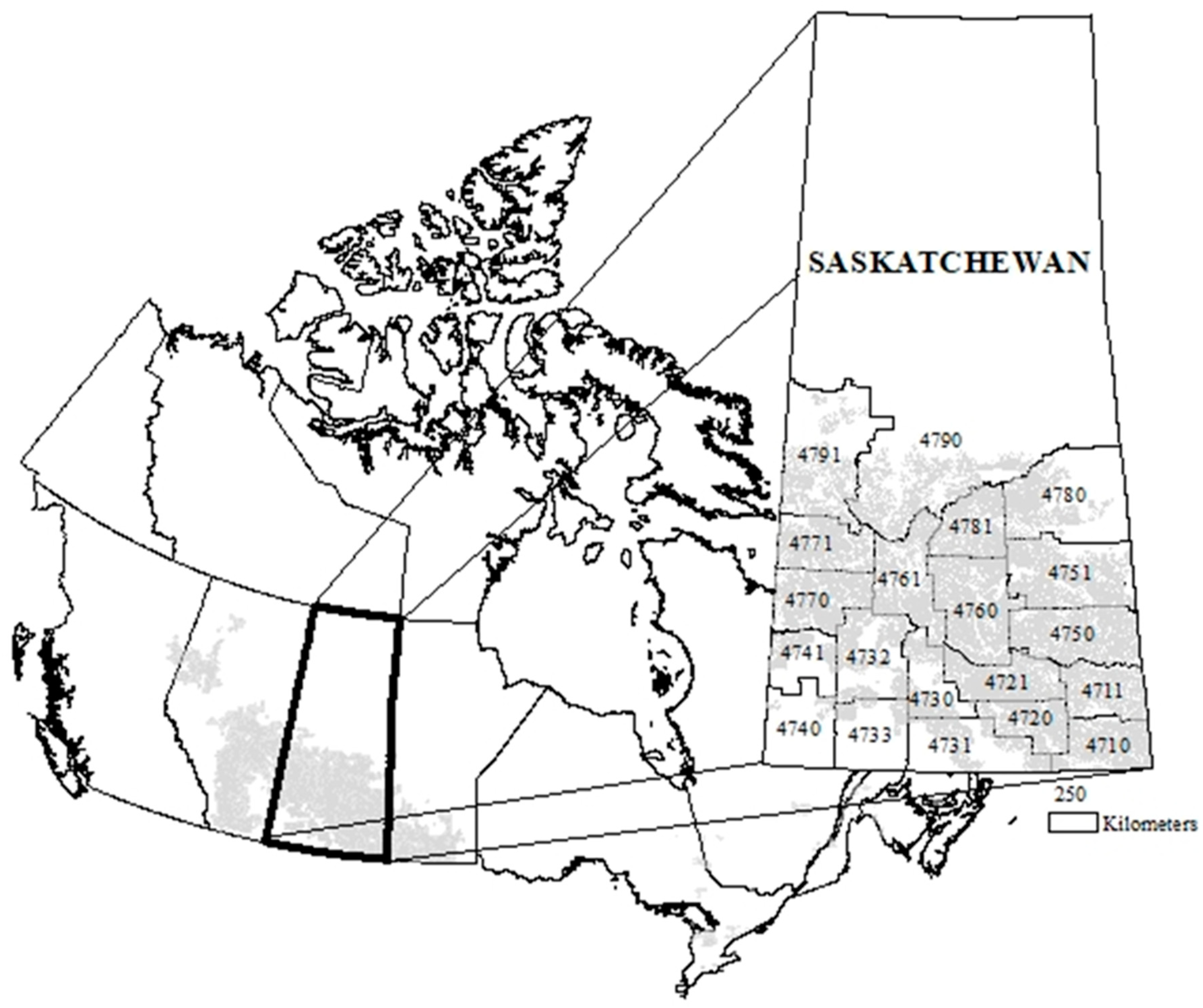
2.1. Study Area
2.2. Soil Moisture Data Sets
2.2.1. SMOS
2.2.2. ESA-CCI
2.2.3. Canadian Meteorological Centre Soil Moisture
2.3. Iterative Chi-Squared Modelling
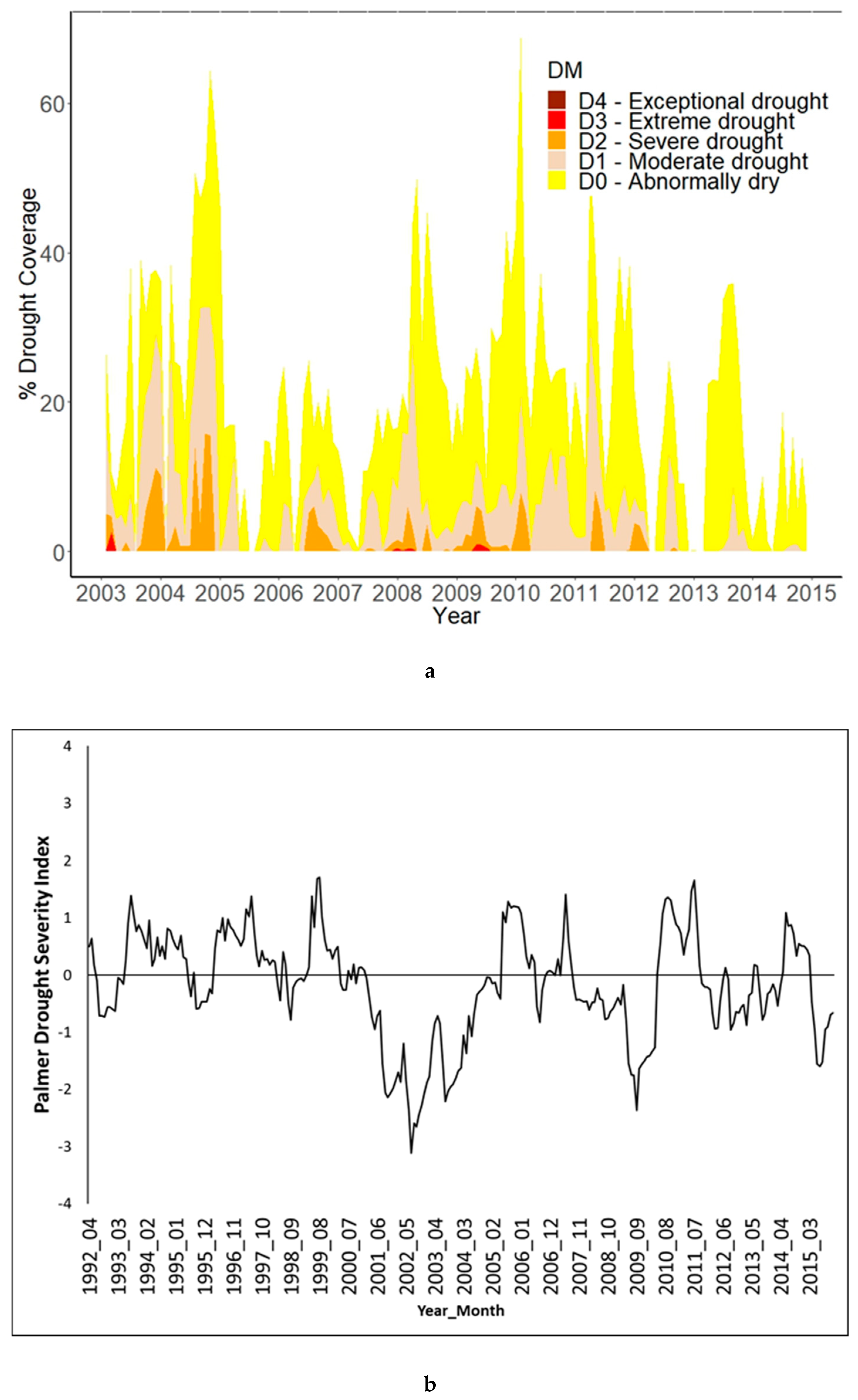
2.4. Climate Conditions
3. Results and Discussion
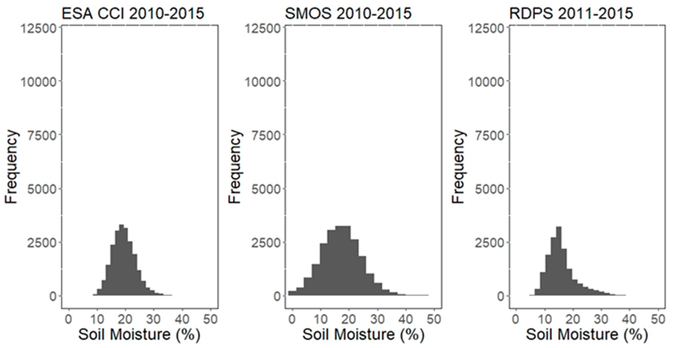
3.1. Soil Moisture Data Characteristics
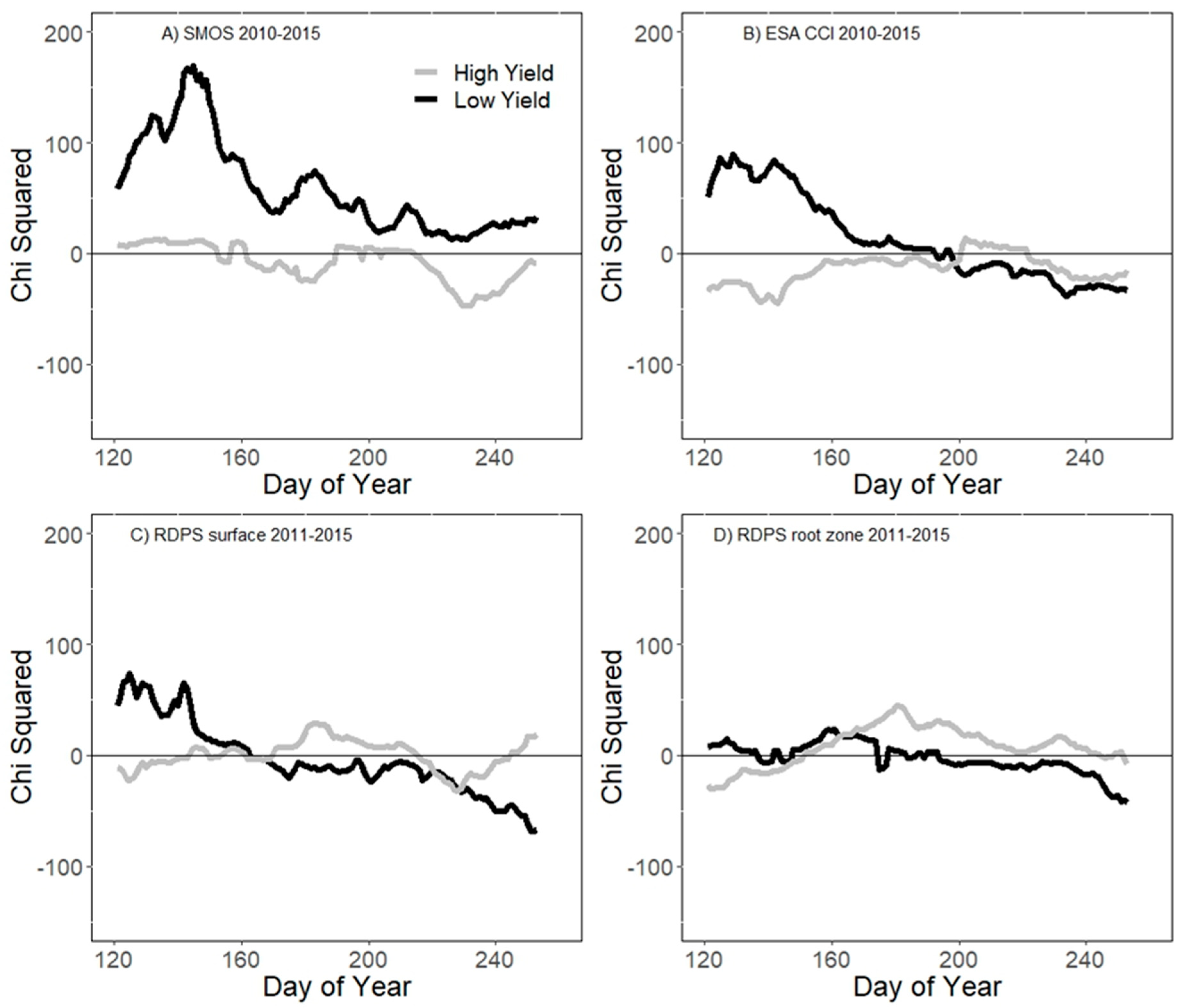
3.2. Impact of Data Type on the Relationship Between Soil Moisture and Canola Yield
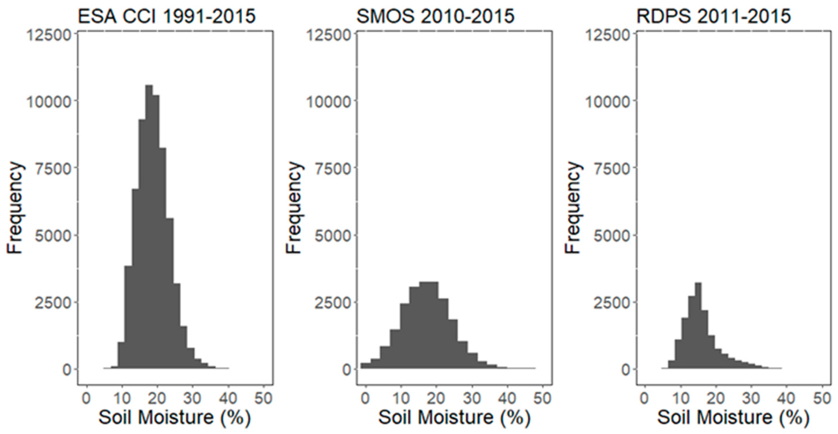
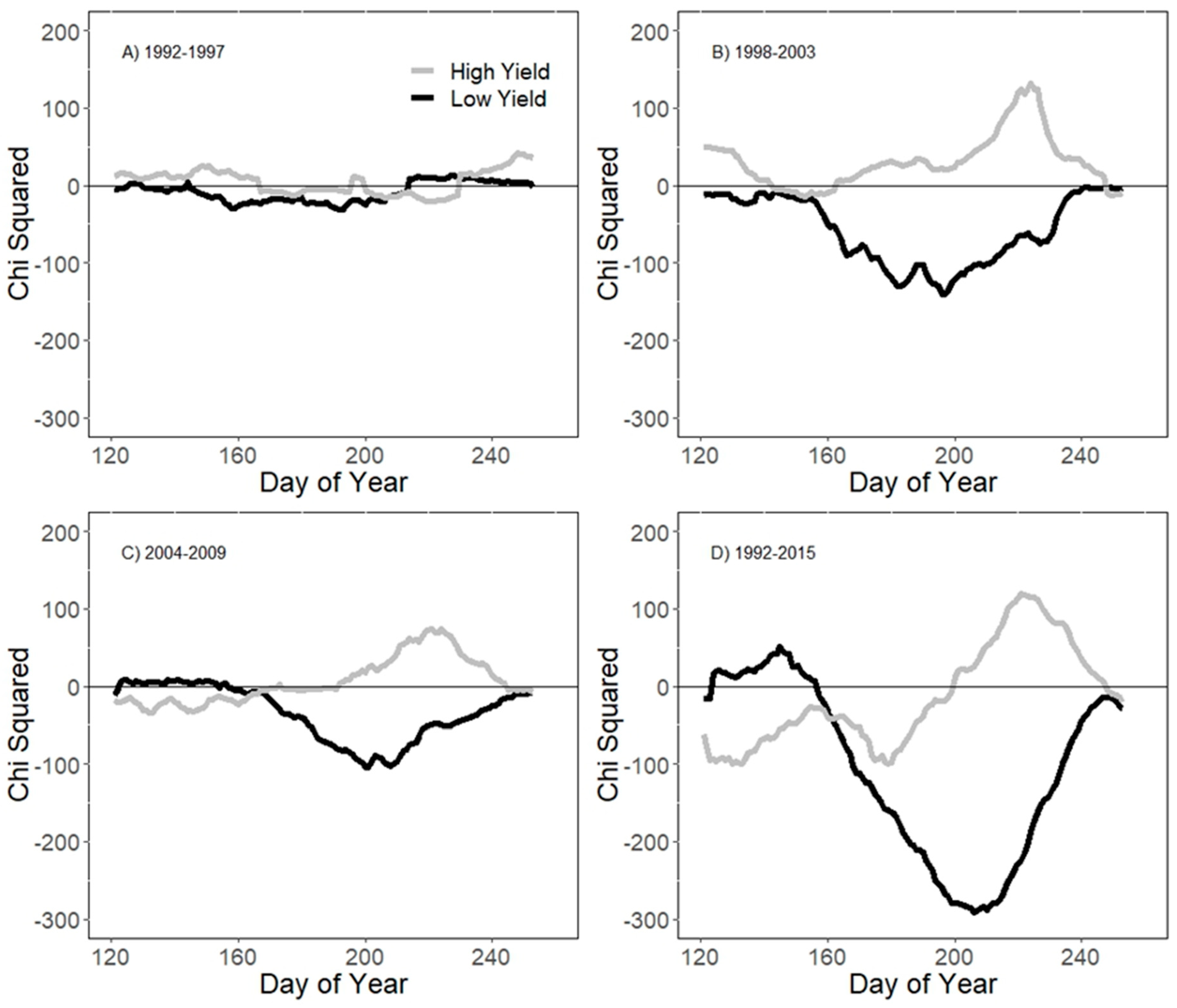
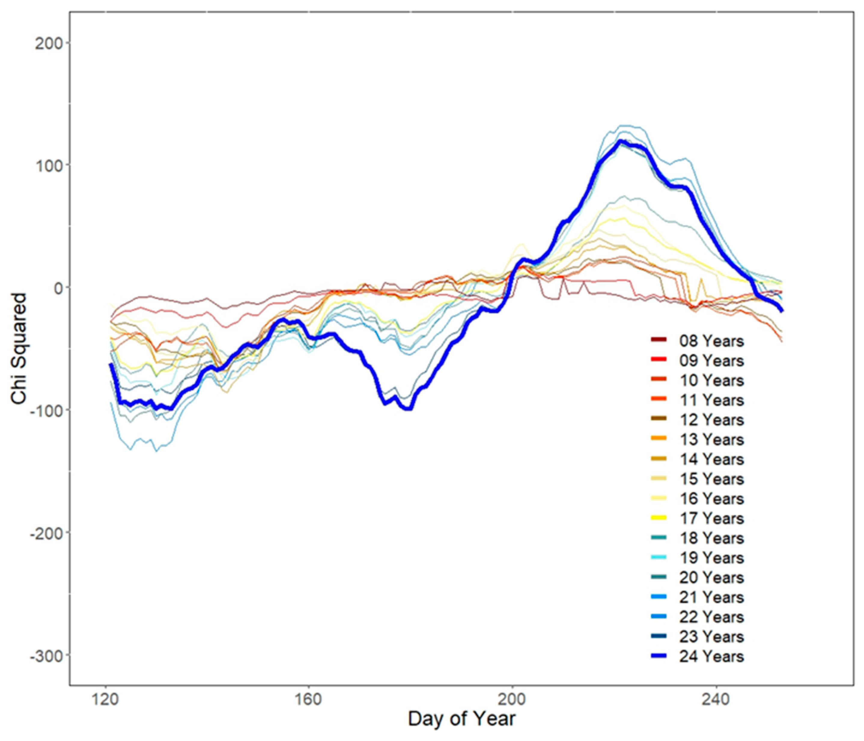
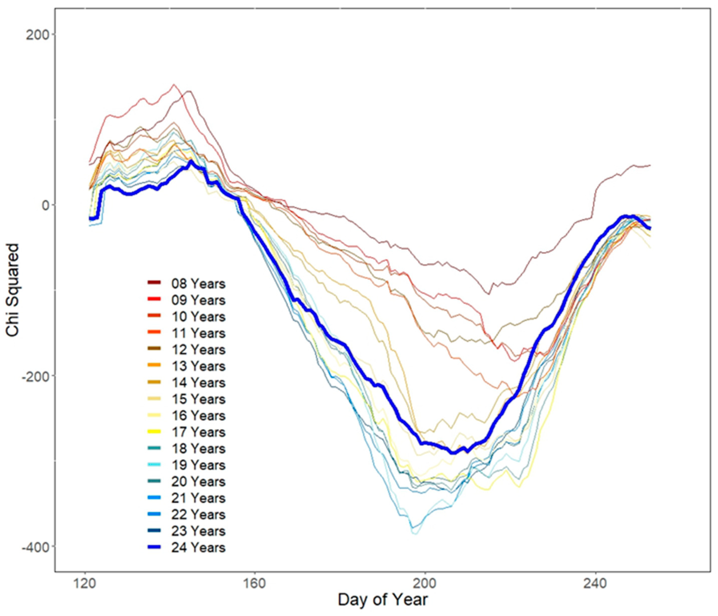
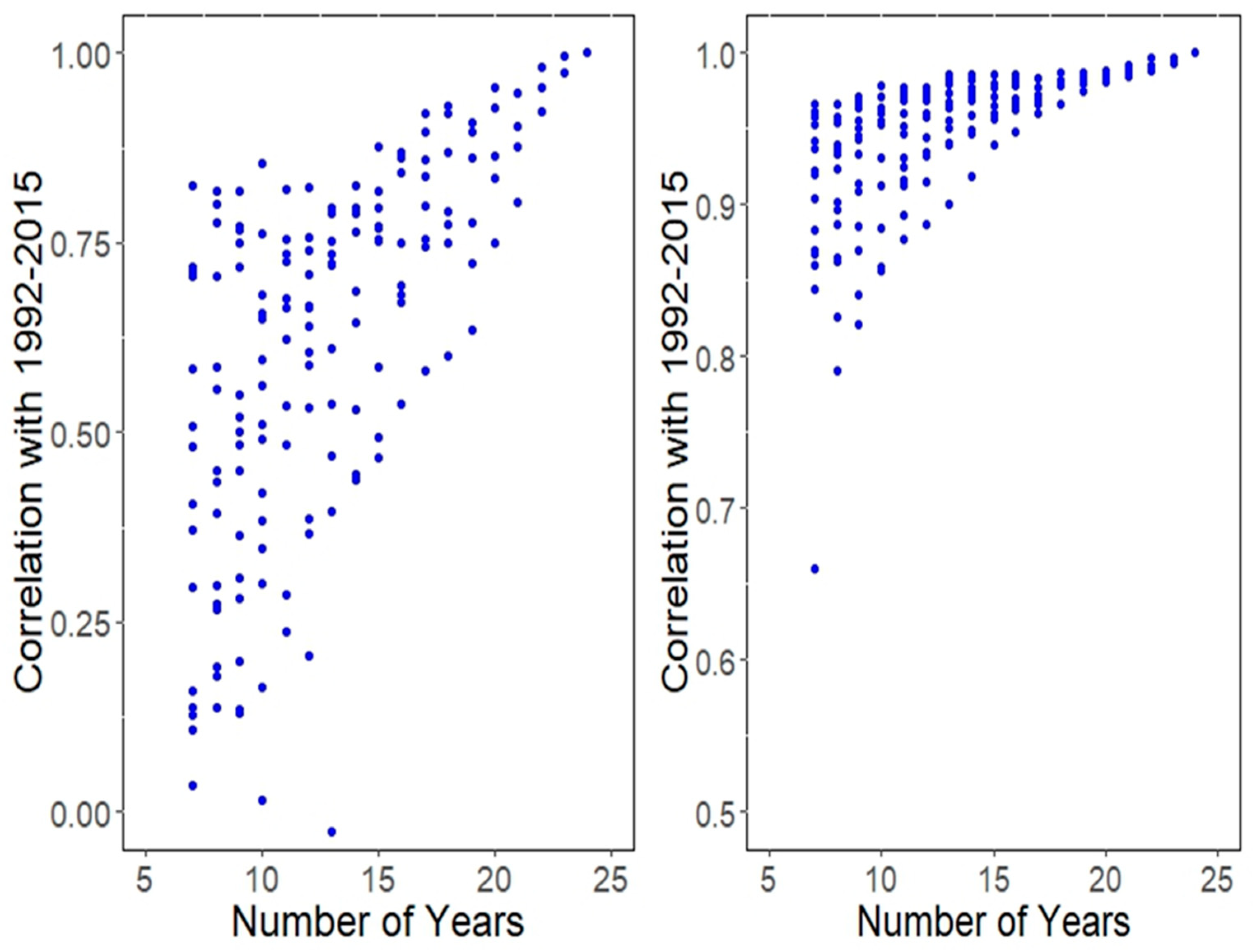
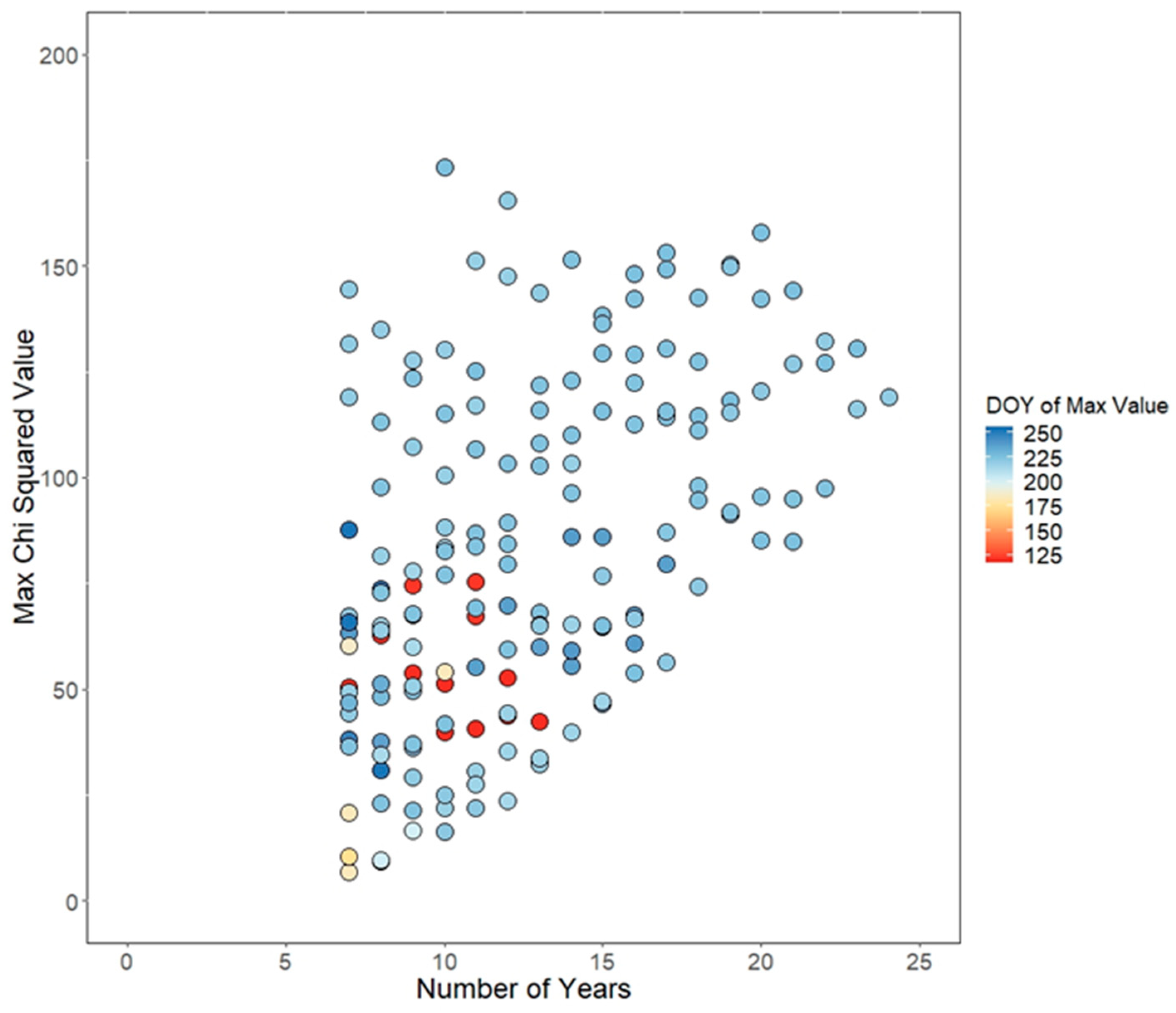
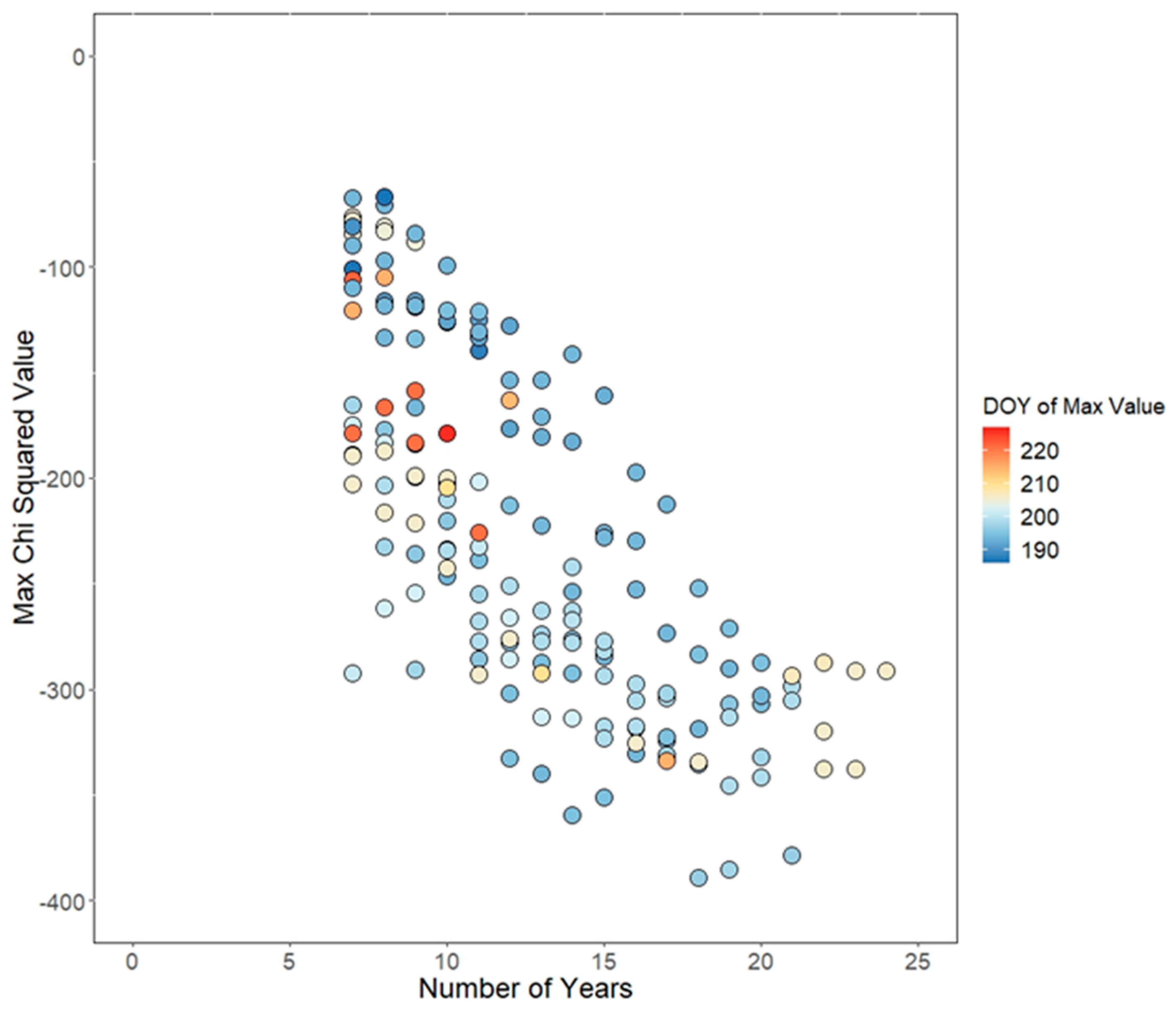
3.3. Impact of Soil Moisture Baseline Length on Impact Assessment
4. Conclusions
Author Contributions
Funding
Acknowledgments
Conflicts of Interest
References
- Palmer, W.C. Keeping Track of Crop Moisture Conditions, Nationwide: The New Crop Moisture Index. Weatherwise 1968, 21, 156–161. [Google Scholar] [CrossRef]
- Quiring, S.M.; Papakryiakou, T.N. An Evaluation of Agricultural Drought Indices for the Canadian Prairies. Agric. For. Meteorol. 2003, 118, 49–62. [Google Scholar] [CrossRef]
- Sheffield, J.; Goteti, G.; Wen, F.H.; Wood, E.F. A Simulated Soil Moisture Based Drought Analysis for the United States. J. Geophys. Res.-Atmos. 2004, 109. [Google Scholar] [CrossRef]
- Champagne, C.; Rowlandson, T.; Berg, A.; Burns, T.; L’Heureux, J.; Tetlock, E.; Adams, J.R.; McNairn, H.; Toth, B.; Itenfisu, D. Satellite Surface Soil Moisture from SMOS and Aquarius: Assessment for Applications in Agricultural Landscapes. Int. J. Appl. Earth Obs. Geoinf. 2016, 45, 143–154. [Google Scholar] [CrossRef]
- Cui, C.; Xu, J.; Zeng, J.; Chen, K.S.; Bai, X.; Lu, H.; Chen, Q.; Zhao, T. Soil Moisture Mapping from Satellites: An Intercomparison of SMAP, SMOS, FY3B, AMSR2, and ESA CCI over Two Dense Network Regions at Different Spatial Scales. Remote Sens. 2018, 10, 33. [Google Scholar] [CrossRef]
- Crow, W.T.; Kumar, S.V.; Bolten, J.D. On the Utility of Land Surface Models for Agricultural Drought Monitoring. Hydrol. Earth Syst. Sci. 2012, 16, 3451–3460. [Google Scholar] [CrossRef]
- Han, E.; Crow, W.T.; Holmes, T.; Bolten, J. Benchmarking a Soil Moisture Data Assimilation System for Agricultural Drought Monitoring. J. Hydrometeorol. 2014, 15, 1117–1134. [Google Scholar] [CrossRef]
- Mishra, A.K.; Singh, V.P. A Review of Drought Concepts. J. Hydrol. 2010, 391, 202–216. [Google Scholar] [CrossRef]
- Heim, R.R. A Review of Twentieth-Century Drought Indices Used in the United States. Bull. Am. Meteorol. Soc. 2002, 83, 1149–1165. [Google Scholar] [CrossRef]
- Champagne, C.; Davidson, A.; Cherneski, P.; L’Heureux, J.; Hadwen, T. Monitoring Agricultural Risk in Canada Using L-band Passive Microwave Soil Moisture from SMOS. J. Hydrometeorol. 2015, 16, 5–18. [Google Scholar] [CrossRef]
- Carrão, H.; Russo, S.; Sepulcre-Canto, G.; Barbosa, P. An Empirical Standardized Soil Moisture Index for Agricultural Drought Assessment from Remotely Sensed Data. Int. J. Appl. Earth Obs. Geoinf. 2016, 48, 74–84. [Google Scholar] [CrossRef]
- Rahmani, A.; Golian, S.; Brocca, L. Multiyear Monitoring of Soil Moisture over Iran through Satellite and Reanalysis Soil Moisture Products. Int. J. Appl. Earth Obs. Geoinf. 2016, 48, 85–95. [Google Scholar] [CrossRef]
- Martínez-Fernández, J.; González-Zamora, A.; Sánchez, N.; Gumuzzio, A.; Herrero-Jiménez, M.C. Satellite Soil Moisture for Agricultural Drought Monitoring: Assessment of the SMOS Derived Soil Water Deficit Index. Remote Sens. Environ. 2016, 177, 277–286. [Google Scholar] [CrossRef]
- Mishra, A.; Vu, T.; Veettil, A.V.; Entekhabi, D. Drought Monitoring with Soil Moisture Active Passive (SMAP) Measurements. J. Hydrol. 2017, 552, 620–632. [Google Scholar] [CrossRef]
- Dorigo, W.; Wagner, W.; Albergel, C.; Albrecht, F.; Balsamo, G.; Brocca, L.; Chung, D.; Ertl, M.; Forkel, M.; Gruber, A.; et al. ESA CCI Soil Moisture for Improved Earth System Understanding: State-of-the Art and Future Directions. Remote Sens. Environ. 2017, 203, 185–215. [Google Scholar] [CrossRef]
- Brocca, L.; Crow, W.T.; Ciabatta, L.; Massari, C.; de Rosnay, P.; Enenkel, M.; Hahn, S.; Amarnath, G.; Camici, S.; Tarpanelli, A.; et al. A Review of the Applications of Ascat Soil Moisture Products. IEEE J. Sel. Top. Appl. Earth Obs. Remote Sens. 2017, 10, 2285–2306. [Google Scholar] [CrossRef]
- Loew, A.; Holmes, T.; de Jeu, R. The European Heat Wave 2003: Early Indicators from Multisensoral Microwave Remote Sensing? J. Geophys. Res.-Atmos. 2009, 114, D05103. [Google Scholar] [CrossRef]
- McNally, A.; Husak, G.J.; Brown, M.; Carroll, M.; Funk, C.; Yatheendradas, S.; Arsenault, K.; Peters-Lidard, C.; Verdin, J.P. Calculating Crop Water Requirement Satisfaction in the West Africa Sahel with Remotely Sensed Soil Moisture. J. Hydrometeorol. 2015, 16, 295–305. [Google Scholar] [CrossRef]
- Tagesson, T.; Horion, S.; Nieto, H.; Zaldo Fornies, V.; Mendiguren González, G.; Bulgin, C.E.; Ghent, D.; Fensholt, R. Disaggregation of SMOS Soil Moisture over West Africa Using the Temperature and Vegetation Dryness Index Based on Seviri Land Surface Parameters. Remote Sens. Environ. 2018, 206, 424–441. [Google Scholar] [CrossRef]
- Eswar, R.; Das, N.N.; Poulsen, C.; Behrangi, A.; Swigart, J.; Svoboda, M.; Entekhabi, D.; Yueh, S.; Doorn, B.; Entin, J. SMAP Soil Moisture Change as an Indicator of Drought Conditions. Remote Sens. 2018, 10, 788. [Google Scholar]
- McNally, A.; Shukla, S.; Arsenault, K.R.; Wang, S.; Peters-Lidard, C.D.; Verdin, J.P. Evaluating ESA CCI Soil Moisture in East Africa. Int. J. Appl. Earth Obs. Geoinf. 2016, 48, 96–109. [Google Scholar] [CrossRef] [PubMed]
- Park, S.; Im, J.; Park, S.; Rhee, J. Drought Monitoring Using High Resolution Soil Moisture through Multi-Sensor Satellite Data Fusion over the Korean Peninsula. Agric. For. Meteorol. 2017, 237–238, 257–269. [Google Scholar] [CrossRef]
- Champagne, C.; Zhang, Y.; Cherneski, P.; Hadwen, T. Estimating Regional Scale Hydroclimatic Risk Conditions from the Soil Moisture Active-Passive (SMAP) Satellite. Geosciences 2018, 8, 127. [Google Scholar] [CrossRef]
- Cammalleri, C.; Vogt, J.V.; Bisselink, B.; De Roo, A. Comparing Soil Moisture Anomalies from Multiple Independent Sources over Different Regions across the Globe. Hydrol. Earth Syst. Sci. 2017, 21, 6329–6343. [Google Scholar] [CrossRef]
- Holgate, C.M.; De Jeu, R.A.M.; Van Dijk, A.I.J.M.; Liu, Y.Y.; Renzullo, L.J.; Dharssi, I.; Parinussa, R.M.; Van Der Schalie, R.; Gevaert, A.; Walker, J.; et al. Comparison of Remotely Sensed and Modelled Soil Moisture Data Sets across Australia. Remote Sens. Environ. 2016, 186, 479–500. [Google Scholar] [CrossRef]
- McKeown, A.; Warland, J.; McDonald, M.R. Long-Term Marketable Yields of Horticultural Crops in Southern Ontario in Relation to Seasonal Climate. Can. J. Plant Sci. 2005, 85, 431–438. [Google Scholar] [CrossRef]
- Kutcher, H.R.; Warland, J.S.; Brandt, S.A. Temperature and Precipitation Effects on Canola Yields in Saskatchewan, Canada. Agric. For. Meteorol. 2010, 150, 161–165. [Google Scholar] [CrossRef]
- White, J.; Berg, A.; Champagne, C.; Warland, J.; Zhang, Y. Canola Yield Sensitivity to Passive Microwave-Derived Soil Moisture Estimates in Saskatchewan, Canada. Agric. For. Meteorol. 2019, in press. [Google Scholar] [CrossRef]
- Campbell, C.A.; Zentner, R.P.; Gameda, S.; Blomert, B.; Wall, D.D. Production of Annual Crops on the Canadian Prairies: Trends during 1976–1998. Can. J. Soil Sci. 2002, 82, 45–57. [Google Scholar] [CrossRef]
- Tadesse, T.; Champagne, C.; Wardlow, B.D.; Hadwen, T.A.; Brown, J.F.; Demisse, G.B.; Bayissa, Y.A.; Davidson, A.M. Building the Vegetation Drought Response Index for Canada (Vegdri-Canada) to Monitor Agricultural Drought: First Results. Gisci. Remote Sens. 2017, 54, 230–257. [Google Scholar] [CrossRef]
- Angadi, S.V.; Cutforth, H.W.; Miller, P.R.; McConkey, B.G.; Entz, M.H.; Brandt, S.A.; Volkmar, K.M. Response of Three Brassica Species to High Temperature Stress during Reproductive Growth. Can. J. Plant Sci. 2000, 80, 693–701. [Google Scholar] [CrossRef]
- Statistics Canada. Field Crop Reporting Series: Estimated Production of Principle Field Crops, Canada. In Field Crop Reporting Series; Minister of Industry, Ed.; Statistics Canada: Ottawa, ON, Canada, 2008; p. 26. [Google Scholar]
- Kerr, Y.H.; Waldteufel, P.; Richaume, P.; Wigneron, J.P.; Ferrazzoli, P.; Mahmoodi, A.; Al Bitar, A.; Cabot, F.; Gruhier, C.; Juglea, S.E.; et al. The SMOS Soil Moisture Retrieval Algorithm. IEEE Trans. Geosci. Remote Sens. 2012, 50, 1384–1403. [Google Scholar] [CrossRef]
- Owe, M.; de Jeu, R.; Walker, J. A Methodology for Surface Soil Moisture and Vegetation Optical Depth Retrieval Using the Microwave Polarization Difference Index. IEEE Trans. Geosci. Remote Sens. 2001, 39, 1643–1654. [Google Scholar] [CrossRef]
- Naeimi, V.; Scipal, K.; Bartalis, Z.; Hasenauer, S.; Wagner, W. An Improved Soil Moisture Retrieval Algorithm for Ers and Metop Scatterometer Observations. IEEE Trans. Geosci. Remote Sens. 2009, 47, 1999–2013. [Google Scholar] [CrossRef]
- Bélair, S.; Brown, R.; Mailhot, J.; Bilodeau, B.; Crevier, L.P. Operational Implementation of the Isba Land Surface Scheme in the Canadian Regional Weather Forecast Model. Part II: Cold Season Results. J. Hydrometeorol. 2003, 4, 371–386. [Google Scholar] [CrossRef]
- Bélair, S.; Crevier, L.P.; Mailhot, J.; Bilodeau, B.; Delage, Y. Operational Implementation of the Isba Land Surface Scheme in the Canadian Regional Weather Forecast Model. Part I: Warm Season Results. J. Hydrometeorol. 2003, 4, 352–370. [Google Scholar] [CrossRef]
- Caprio, J.M.; Quamme, H.A.; Redmond, K.T. A Statistical Procedure to Determine Recent Climate Change of Extreme Daily Meteorological Data as Applied at Two Locations in Northwestern North America. Clim. Chang. 2009, 92, 65–81. [Google Scholar] [CrossRef]
- Kalma, J.; Laughlin, G.P.; Caprio, J.M.; Hamer, P.J.C. Weather and Winterkill of Wheat: A Case Study. In The Bioclimatology of Frost; Kalma, J., Ed.; Springer: Berlin, Germany, 1992; pp. 73–82. [Google Scholar]
- Caprio, J.M.; Quamme, H.A. Weather Conditions Associated with Grape Production in the Okanagan Valley of British Columbia and Potential Impact of Climate Change. Can. J. Plant Sci. 2002, 82, 755–763. [Google Scholar] [CrossRef]
- Caprio, J.M.; Quamme, H.A. Weather Conditions Associated with Apple Production in the Okanagan Valley of British Columbia. Can. J. Plant Sci. 1999, 79, 129–137. [Google Scholar] [CrossRef]
- McKeown, A.W.; Warland, J.; McDonald, M.R. Long-Term Climate and Weather Patterns in Relation to Crop Yield: A Minireview. Can. J. Bot.-Rev. Can. Bot. 2006, 84, 1031–1036. [Google Scholar] [CrossRef]
- Caprio, J.M.; Fritts, H.C.; Holmes, R.L.; Meko, D.M.; Hemming, D.L. A Chi-Square Test for the Association and Timing of Tree Ring-Daily Weather Relationships: A New Technique for Dendroclimatology. Tree-Ring Soc. 2003, 59, 99–113. [Google Scholar]
- Powell, L.R.; Berg, A.A.; Johnson, D.L.; Warland, J.S. Relationships of Pest Grasshopper Populations in Alberta, Canada to Soil Moisture and Climate Variables. Agric. For. Meteorol. 2007, 144, 73–84. [Google Scholar] [CrossRef]
- National Agroclimate Information Service. Drought Watch. Agriculture and Agri-Food Canada. Available online: http://www.agr.gc.ca/eng/programs-and-services/drought-watch/?id=1461263317515 (accessed on 12 November 2018).
- Akinremi, O.O.; McGinn, S.M.; Barr, A.G. Evaluation of the Palmer Drought Index on the Canadian Prairies. J. Clim. 1996, 9, 897–905. [Google Scholar] [CrossRef] [Green Version]
- Chipanshi, A.C.; Warren, R.T.; L’Heureux, J.; Waldner, D.; McLean, H.; Qi, D. Use of the National Drought Model (NDM) in Monitoring Selected Agroclimatic Risks across the Agricultural Landscape of Canada. Atmos. Ocean 2013, 51, 471–488. [Google Scholar] [CrossRef]
- Carrera, M.; Charpentier, D.; Belair, S.; Zhang, S.; Bilodeau, B. Downscaling SMOS Brightness Temperatures to Produce Higher Resolution Soil Moisture Analyses. In Proceedings of the IEEE International Geoscience and Remote Sensing Symposium, Quebec City, QC, Canada, 13–18 July 2014. [Google Scholar]
- Husain, S.Z.; Alavi, N.; Bélair, S.; Carrera, M.; Zhang, S.; Fortin, V.; Abrahamowicz, M.; Gauthier, N. The Multibudget Soil, Vegetation, and Snow (Svs) Scheme for Land Surface Parameterization: Offline Warm Season Evaluation. J. Hydrometeorol. 2016, 17, 2293–2313. [Google Scholar] [CrossRef]
- Escorihuela, M.J.; Chanzy, A.; Wigneron, J.P.; Kerr, Y.H. Effective Soil Moisture Sampling Depth of L-band Radiometry: A Case Study. Remote Sens. Environ. 2010, 114, 995–1001. [Google Scholar] [CrossRef]


| N | Mean | Sd | Median | Skew | Kurtosis | |
|---|---|---|---|---|---|---|
| RDPS surface 2011–2015 | 15300 | 16.0 | 5.1 | 15.2 | 1.2 | 1.8 |
| SMOS 2010–2015 | 21410 | 17.3 | 7.1 | 17.2 | 0.2 | 0.3 |
| ESA CCI 2010–2015 | 18349 | 19.6 | 4.1 | 19.3 | 0.4 | 0.4 |
| ESA CCI 1992–2015 | 61770 | 18.9 | 4.5 | 18.6 | 0.5 | 0.3 |
| ESA CCI 1992–1997 | 7990 | 19.2 | 4.9 | 19.1 | 0.4 | 0.3 |
| ESA CCI 1998–2003 | 12873 | 17.7 | 4.9 | 17.1 | 0.7 | 0.6 |
| ESA CCI 2004–2009 | 18208 | 18.8 | 4.3 | 18.4 | 0.5 | 0.2 |
| RDPS rootzone 2011–2015 | 15300 | 17.6 | 2.8 | 17.7 | −0.4 | 1.3 |
© 2019 by the authors. Licensee MDPI, Basel, Switzerland. This article is an open access article distributed under the terms and conditions of the Creative Commons Attribution (CC BY) license (http://creativecommons.org/licenses/by/4.0/).
Share and Cite
Champagne, C.; White, J.; Berg, A.; Belair, S.; Carrera, M. Impact of Soil Moisture Data Characteristics on the Sensitivity to Crop Yields Under Drought and Excess Moisture Conditions. Remote Sens. 2019, 11, 372. https://doi.org/10.3390/rs11040372
Champagne C, White J, Berg A, Belair S, Carrera M. Impact of Soil Moisture Data Characteristics on the Sensitivity to Crop Yields Under Drought and Excess Moisture Conditions. Remote Sensing. 2019; 11(4):372. https://doi.org/10.3390/rs11040372
Chicago/Turabian StyleChampagne, Catherine, Jenelle White, Aaron Berg, Stephane Belair, and Marco Carrera. 2019. "Impact of Soil Moisture Data Characteristics on the Sensitivity to Crop Yields Under Drought and Excess Moisture Conditions" Remote Sensing 11, no. 4: 372. https://doi.org/10.3390/rs11040372