On-Board Georeferencing Using FPGA-Based Optimized Second-Order Polynomial Equation
by
Dequan Liu
1,3, 
Guoqing Zhou
1,2,3,4,*,
Jingjin Huang
2,3,
Rongting Zhang
2,3,
Lei Shu
2,3,
Xiang Zhou
1,4 and
Chun Sheng Xin
5 1
School of Microelectronics, Tianjin University, Tianjin 300072, China
2
School of Precision Instrument & Opto-Electronics Engineering, Tianjin University, Tianjin 300072, China
3
The Center for Remote Sensing, Tianjin University, Tianjin 300072, China
4
GuangXi Key Laboratory for Spatial Information and Geomatics, Guilin University of Technology, Guilin 541004, China
5
Department of Electrical and Computer Engineering, Old Dominion University, Norfolk, VA 23529, USA
*
Author to whom correspondence should be addressed.
Remote Sens. 2019, 11(2), 124; https://doi.org/10.3390/rs11020124
Submission received: 27 November 2018
/
Revised: 28 December 2018
/
Accepted: 3 January 2019
/
Published: 10 January 2019
(This article belongs to the Special Issue Real-Time Processing of Remotely-Sensed Imaging Data)
Abstract
:For real-time monitoring of natural disasters, such as fire, volcano, flood, landslide, and coastal inundation, highly-accurate georeferenced remotely sensed imagery is needed. Georeferenced imagery can be fused with geographic spatial data sets to provide geographic coordinates and positing for regions of interest. This paper proposes an on-board georeferencing method for remotely sensed imagery, which contains five modules: input data, coordinate transformation, bilinear interpolation, and output data. The experimental results demonstrate multiple benefits of the proposed method: (1) the computation speed using the proposed algorithm is 8 times faster than that using PC computer; (2) the resources of the field programmable gate array (FPGA) can meet the requirements of design. In the coordinate transformation scheme, 250,656 LUTs, 499,268 registers, and 388 DSP48s are used. Furthermore, 27,218 LUTs, 45,823 registers, 456 RAM/FIFO, and 267 DSP48s are used in the bilinear interpolation module; (3) the values of root mean square errors (RMSEs) are less than one pixel, and the other statistics, such as maximum error, minimum error, and mean error are less than one pixel; (4) the gray values of the georeferenced image when implemented using FPGA have the same accuracy as those implemented using MATLAB and Visual studio (C++), and have a very close accuracy implemented using ENVI software; and (5) the on-chip power consumption is 0.659W. Therefore, it can be concluded that the proposed georeferencing method implemented using FPGA with second-order polynomial model and bilinear interpolation algorithm can achieve real-time geographic referencing for remotely sensed imagery.
1. Introduction
With the advancement of technological, remote sensing (RS) images are becoming more widely used in natural disasters monitoring and positioning [1,2,3]. They are required to rapidly produce highly accurate georeferenced image. However, the processing speed of the traditional methods for indirect georeferencing of RS images cannot to meet the timeliness requirements [4,5,6,7,8,9]. Therefore, it would be highly desirable to develop a rapid, inexpensive technique to implement an on-board georeferencing. This paper proposes a georeferencing method based onfield programmable gate arrays (FPGAs) with the optimized second-order polynomial equation and bilinear interpolation scheme.
Georeferencing is a key step in geometric correction which aims to establish the relationship between image coordinates and ground coordinates through various function, such as collinearity equation models (CEM), polynomial function models (PFM), rational function models (RFM), and direct linear transformation models (DLT) [10,11,12,13,14,15]. However, these traditional algorithms were developed for serial instruction systems based on personal computers (PC). As such, these systems hardly meet response time demands of time-critical disasters [5].
To solve the limitation of the speed of RS images processing, many researchers proposed effective alternative processing methods. High-performance computing (HPC) was widely used in RS data processing system. Cluster computing has already offered access to greatly increased computational power at a low cost in a few hyperspectral imaging applications [16,17,18]. Although the algorithms of RS data processing generally map quite nicely to multi-processor systems composed of clusters or networks of CPUs, these systems are usually expensive and difficult to adapt to the on-board RS data processing scenarios. For these reasons, the specialized integrated hardware devices of low weight and low power consumption are essential to reduce mission payload and obtain analysis results in real-time. FPGAs and graphics processing units (GPUs) exhibit good potential to allow for on-board real-time analysis of RS data. Fang et al. [19] presented near real-time approach for CPU/GPU based preprocessing of ZY-3 satellite images. Van et al. [20] proposed a new method to generate undistorted images by implementing the required distortion correction algorithm on a commercial GPU. Thomas et al. [21] described the georeferencing of an airborne hyperspectral imaging system based on pushbroom scanning. Reguera et al. [22] presented a method for real-time geo-correction of images from airborne pushbroom sensors using the hardware acceleration and parallel computing characteristics of modern GPU. López-Fandiño et al. [23] proposed a parallel function with GPU to accelerate the extreme learning machine (ELM) algorithm which is performed on RS data for land cover applications and achieved competitive accuracy results. Lu et al. [24] mapped the fusion method of RS images to GPU. The result shown that the image fusion speed based on GPU was much quicker than that based on CPU when the image size was getting bigger. Now, the use of GPUs to accelerate RS processing has resulted in further related research achievements. However, most parallel processing methods based on GPU multitasking are not alone capable of surmounting the shortcomings of serial instrument methods [25,26]. Additionally, FPGAs exhibit lower power dissipation figures than GPUs [27]. FPGAs have been consolidated as the standard choice for on-board RS data processing due to their smaller size, weight, and power consumption when compared to other HPC systems [27,28,29,30,31,32]. Zhou et al. [28] presented the concept of the “on-board processing system”. Huang et al. [29] proposed an FPGA architecture that consisted of corner detection, corner matching, outlier rejection, and sub-pixel precision localization. Pakartipangi et al. [30] analyzed the camera array on-board data handling using an FPGA for nano-satellite application. Huang et al. [31] proposed a new FPGA architecture that considered the reuse of sub-image data. Yu et al. [32] presented a new on-board image compression system architecture for future disaster monitoring by low-earth-orbit (LEO) satellites. Zhou et al. [5] proposed an on-board ortho-rectification for remote sensing images based on an FPGA. Qi et al. [7] presented an FPGA and digital singnal processor (DSP) co-processing system for an optical RS images preprocessing algorithm. Long et al. [33] focused on an automatic matching technique for the specific task of georeferencing RS images and presented a technical frame to match large RS images efficiently using the prior geometric information of the images. Williams et al. [34] discussed the design and implementation of a real-time cloud detection system for on-board RS platform. González et al. [35] presented an N-finder (N-FINDR) algorithm implementation using FPGA for hyperspectral image analysis.
This paper presents an on-board georeferencing scheme using FPGA for remote sensing images. By decomposing the georeferencing algorithm, the proposed georeferencing platform integrates three modules: a data memory, coordinate transformation (including the transformation from geodetic coordinates to the raw image coordinates and the raw image coordinates to the scanning coordinates), and bilinear interpolation. The contributions are summarized as follows.
(1) An optimized second-order polynomial equation and bilinear interpolation are proposed for on-board georeferencing for remotely sensing imagery. (2) An architecture for floating-point block Lower-Upper (LU) decomposition is designed to solve the inverse for large-sized matrices. (3)To reduce resource consumption, some strategies are adopted in FPGA implementation, i.e., 32-bit integer and floating-point mixed operation and serial-parallel data communication.
The remainder of the paper is organized as follows. Section 2 reviews the traditional second-order polynomial georeferencing algorithm, bilinear interpolation method and optimizes the algorithms based on the FPGA; Section 3 gives the details of the implementation using FPGA for the georeferencing scheme; Section 4 describes and validates the experimental results. The conclusion is presented in Section 5.
2. Optimization for Georeferencing Scheme
The georeferencing scheme includes the selection of a suitable mathematical distortion model, coordinate transformation, and resampling (interpolation) [36,37,38]. The georeferencing scheme can be classified into direct and indirect methods. The direct method applies the raw image coordinates to compute the georeferenced coordinates, and the indirect method applies the georeferenced image coordinates to compute the raw image coordinates. In this paper, the indirect method is used to establish the relationship of coordinate by the second-order polynomial equations.
2.1. A Brief Review of Georeferencing
2.1.1. Traditional Second-Order Polynomial Equations
The second-order polynomial equations are expressed as follows [39,40,41,42]:
where are the coordinates of the raw image, are the corresponding ground coordinates (longitude, latitude), and and (i = 0, 1, …, 5) are the unknown coefficients of the second-order polynomial equation. After choosing a suitable mathematical distortion model, the unknown coefficients and can be obtained from Equations (1) and (2) with the ground control points (GCPs). GCPs are an important parameter in the geometric calibration, which affect the accuracy of subsequent correction [43]. To ensure accuracy, ten GCPs are selected in the study area. Let the coordinate pairs of ten GCPs can be represented as: , , …, . The matrix form of Equation (1) can be expressed as:
According to the least square method [5], Equation (3) can be simplified as Equation (4).
where is the matrix of the ground coordinates of GCPs, is the coefficients matrix of the second-order polynomial Equation (1), is the coordinates matrix of GCPs in the raw image, and P is the weight matrix. , , and are expressed by Equation (5) through Equation (8).
Typically, the weight of each GCPs is the same. So, . Equation (4) can be descripted as:
In the same way, the coefficients of can be solved by the formula .
2.1.2. Coordinate Transformation
After establishing the second-order polynomial equation and solving the coefficients of Equations (1) and (2), the raw image can be georeferenced pixel-to-pixel. The steps are as follows [44]:
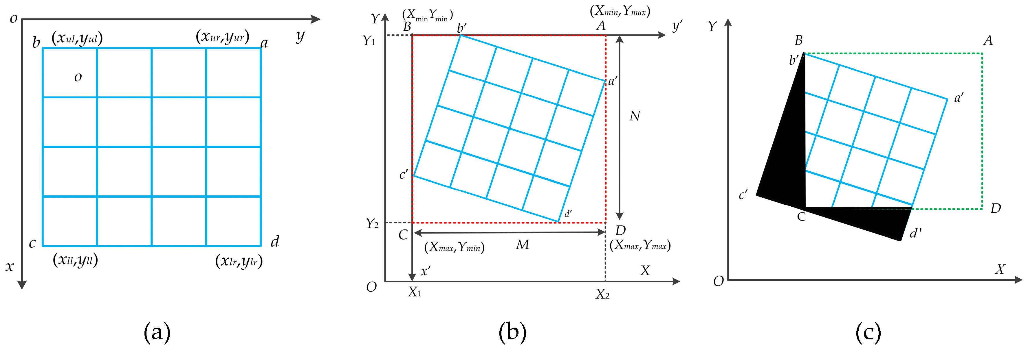
1. The Size of the Georeferenced Image
To properly obtain the georeferenced image, the storage area of georeferenced image must be computed in advance, as shown in Figure 1 [7]. is the raw image, with corners , , , and in the image coordinate system in the Figure 1a. Figure 1b shows the correct range of output image. is the georeferenced image with corners , , and in the ground coordinate system, and is the storage area for georeferenced image. Obviously, if the storage range is not correctly defined, the georeferenced image is improper with a large blank area, as shown in Figure 1c. Therefore, the right boundary should include the entire georeferenced image with minimum exterior blank rectangle as possible.
2. Coordinates of the Four Corners
, , , and are the coordinates of the four corner in the raw image (input image), , , , and are the corresponding ground coordinates of the georeferenced image. The maximum and minimum ground coordinates of the storage area for the georeferenced image (, , , and ) are calculated from the , , , and .
3. Row () and Column () of the Georeferenced Image.
and can be solved by Equation (11).
where and are the ground-sampling distances (GSD) of the output image. Hence, the location of pixel can be described by the row and column in the coordinate system ( 1, 2, 3, …, ; 1, 2, 3, …, ).
4. Coordinate Transformation.
The georeferenced model only expresses the relationship between the ground coordinates and the coordinates of the raw image. To further express the relationship between the raw image coordinates and scanning coordinates of the georeferenced image, it is necessary to convert the ground coordinate into the row and column of georeferenced image, as shown in Equation (12).
where and are the row and column of the georeferenced image, respectively, and are the corresponding ground coordinate.
2.1.3. Resample
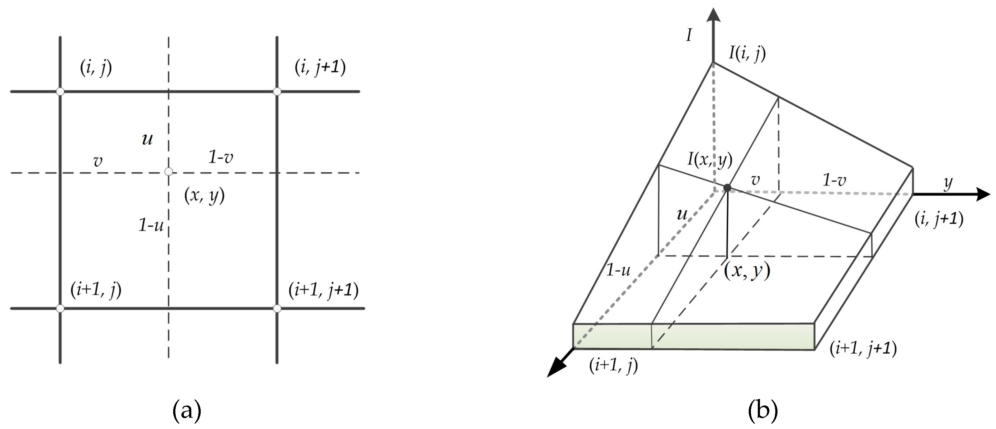
As to be expected, the defined grid center from the georeferenced image will not usually project to the center location of pixel in the raw image after coordinate transformation. To solve this problem, nearest-neighbor interpolation, bilinear interpolation, and cubic interpolation [45] are commonly used. To balance the accuracy and complexity of the preprocessing function, bilinear interpolation is chosen in this paper. The algorithm obtains the pixel value by taking a weighted sum of the pixel values of the four nearest neighbors surrounding the calculated location [46], as shown in Figure 2 and Equation (13).
where, are the coordinates of the georeferenced image, is the gray value of a pixel with coordinates in the georeferenced image; and are the integer part of the corresponding coordinate in the raw image, respectively; and are the fractional parts of the corresponding coordinate in the raw image, respectively. is the gray value of coordinates in the raw image.
2.2. Optimized Georeferencing Scheme
2.2.1. Optimized Second-Order Polynomial Model
To parallel implement the Equations (1) and (2), the second-order polynomial equations are optimized to Equations (14) and (15).
where, , , , and .
In Equation (1), eight multipliers and five adders are required to complete a transformation. However, in Equation (14), five multipliers and five adders are required to complete a transformation. Comparatively, six multipliers are reduced in all. The multipliers and adders required to complete the coordinate transformation are in Table 1.
2.2.2. Optimized Bilinear Interpolation
Equation (13) appears to require eight multiplications, but careful factorization to exploit separability can reduce the multiplication by three [47].
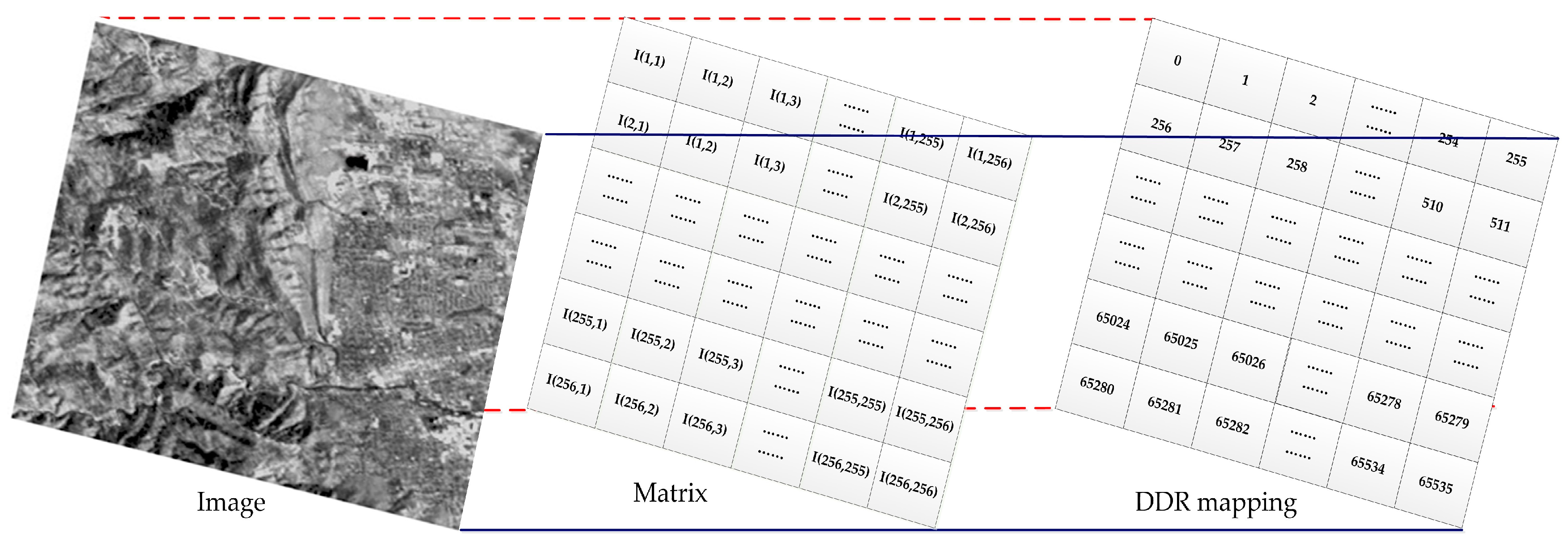
To compute the Equation (16), the gray values of four nearest-neighbors must be read from the memory. The principle of the mapping storage method is to optimize and balance the line and block data access rate [7]. In order to improve memory access efficiency, a multi-array memory storage method is designed in Figure 3. The RS image size is . As such, memory units are designed in double data rate (DDR). The relationship between the address of DDR and coordinates can be described by Equation (17).
where, and are the row and column of the raw image, respectively. is the corresponding address of memory.
3. FPGA-Based Implementation of the Georeferencing Scheme
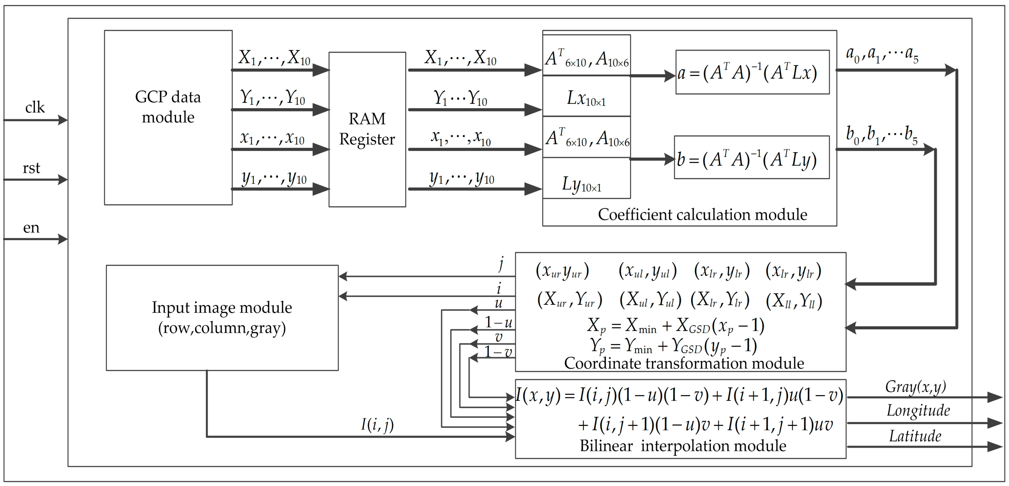
An FPGA hardware architecture is designed for georeferenced of the remotely sensed imagery as shown in Figure 4, which contains five modules: (I) GCP data module; (II) input image module (IIM); (III) coefficient calculation module (CCM); (IV) coordinate transformation module (CTM); and (V) bilinear interpolation module (BIM). The details of five modules are described as follows.
- The GCPs data is stored in the RAM of the GCP data module. These parameters are sent to the CCM, when the enable signal is being received.
- The gray values of the input image are saved to the ROM through the IIM, when the enable signal is being received.
- The coefficients of , , , , , , , , , , and are calculated in the CCM when the GCP data are arrived. The matrices , , , and are parallel computed.
- The coordinate transformation is carried out in the CTM when the coefficients of second-order polynomial equation are arrived. The values of , , , , and are simultaneously sent to the BIM.
- According to Equations (13) and (16), the interpolation values are calculated. At last, the gray values, latitude, and longitude of the georeferenced image are outputted at the same clock cycle.
3.1. FPGA-Based Solution of the Second-Order Polynomial Equation
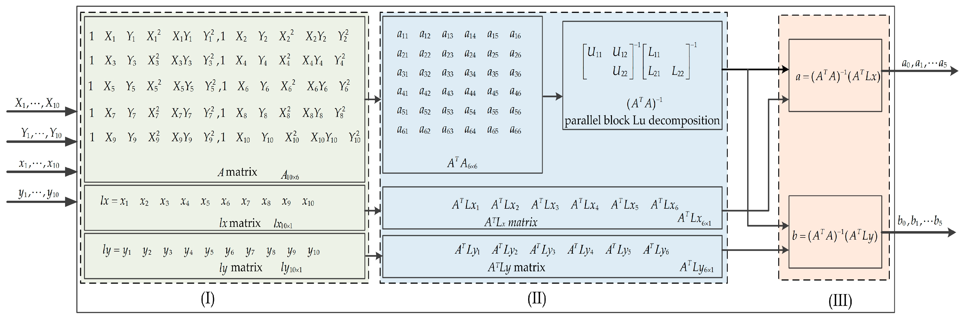
To implement the second-order polynomial equation based on an FPGA, the processing of solving the coefficient is decomposed into three modules (as shown in Figure 5): (I) Form the matrices , , and ; (II) Calculate , , , and , and (III) perform and .
3.1.1. Calculation of Matrix
According to Equation (9) and the principle of matrix multiplication, the coefficients of (1, 2, …, 6) are calculated, as shown in Equations (18) and (19).
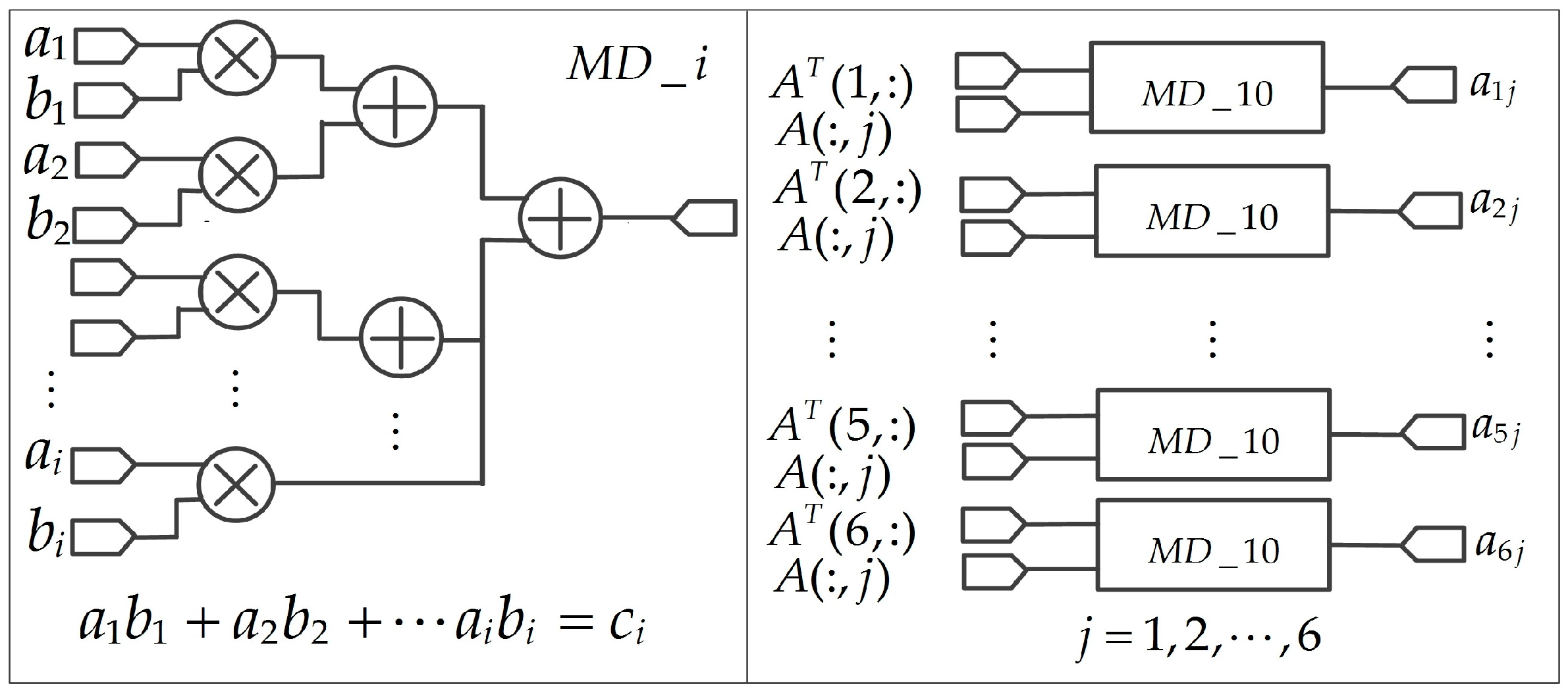
Generally, ten multipliers and nine adders are needed to compute . Therefore, it takes about 324 additions and 360 multiplications to calculate all coefficients. However, the resources are limited on an FPGA chip. Therefore, a combination of serial and parallel strategy is adopted [48,49]. To improve the processing speed, multiplier-adder (MD) modules are used. At the same way, the other coefficients of , , , , , and ( 1, 2, 3, …, 6) are parallel computed at the same clock cycle. Figure 6 shows the architecture of ATA based on an FPGA.
.
3.1.2. LU Decomposition of the Matrix
The coefficient accuracy of the second-order polynomial equation is crucial to the entire system. This paper proposes a parallel structure that uses the floating-point block LU decomposition to solve the inverse of . The matrix can be represented as four matrices , , , and [48, 49, 50, 51], as shown in Equation (20).
where , , , , and are matrices; and are lower triangular matrices, and are upper triangular matrices. From Equation (20), some additional equations can be achieved:
The steps of LU decomposition are as follows.
Step 1: is performed by block LU decomposition; and are obtained.
Step 2: From Equation (22), can be solved by Equation (25):
Step 3: From Equation (23), can be calculated by the product of and (see Equation (26)):
Step 4: matrix is performed by LU decomposition; and matrices are obtained.
1. FPGA-Based Parallel Computation for the LU Decomposition of Matrix
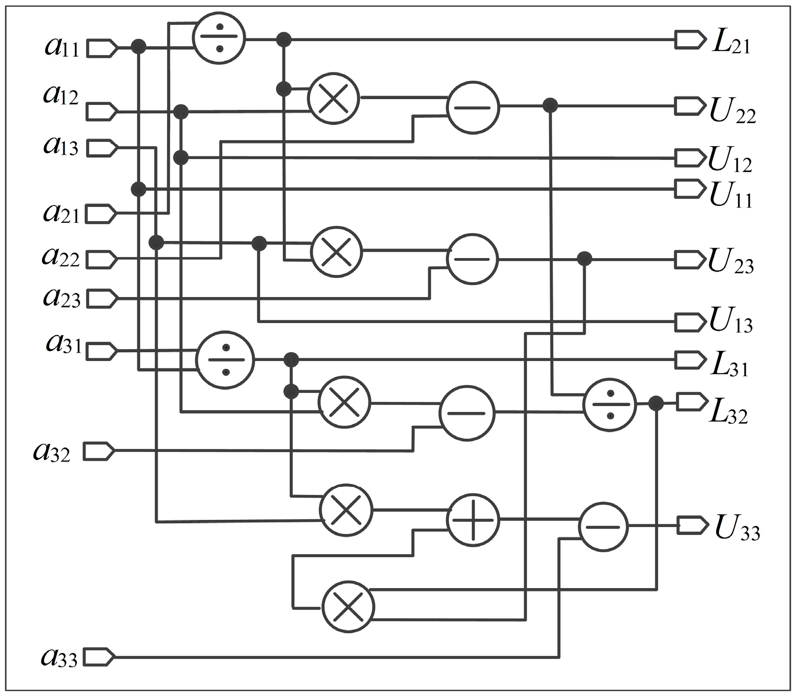
To implement the LU decomposition of matrix on the FPGA, Equation (21) can be modified as Equation (27). The steps of the LU decomposition of matrix are as follows.
Step 1. , , , , , .
Step 2. , .
Step 3. .
Step 4. .
According to Equation (27), a parallel computation architecture for matrices and is presented in Figure 7. Five multipliers, three divisors, one adder, and four subtractors are used. Additionally, some control signals are used to ensure that the results are outputted at the same clock cycle.
2. FPGA-Based Parallel Computation for Matrices and
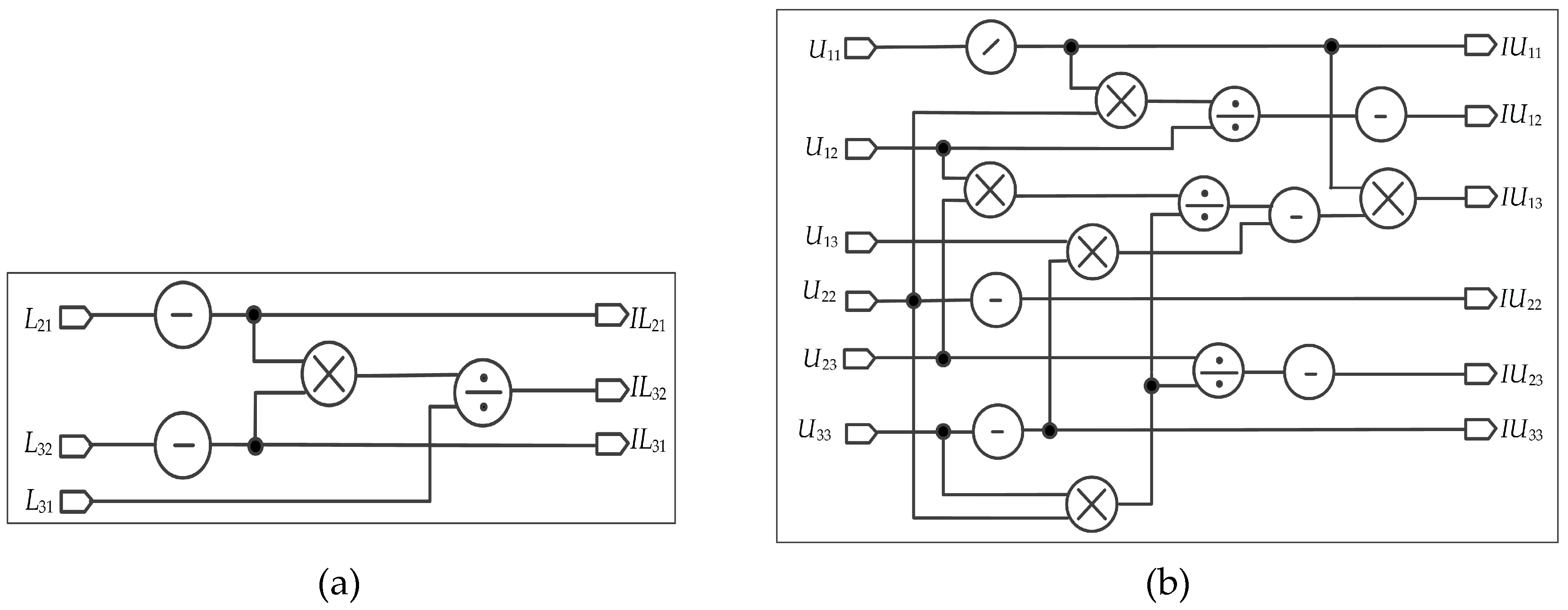
It is well known that the inverse of a lower triangular matrix is another lower triangular matrix, and the inverse of an upper triangular matrix is also another upper triangular matrix. The inversion of matrices and can be rewritten as Equations (28) and (29), respectively.
where , , and .
where , , , , , and .
The parallel computation structures for calculating and are shown in Figure 8. Six multipliers, four divisors, one subtractor (“—” in the circle), and three reciprocals (“/” in the circle) are used. The reverse operation (“-” in the circle) for floating-point is simply to reverse the symbol bit and require very few resources. Additionally, some control signals are used to ensure that the results are outputted at the same clock cycle.
3. FPGA-Based Implementation of Matrices and
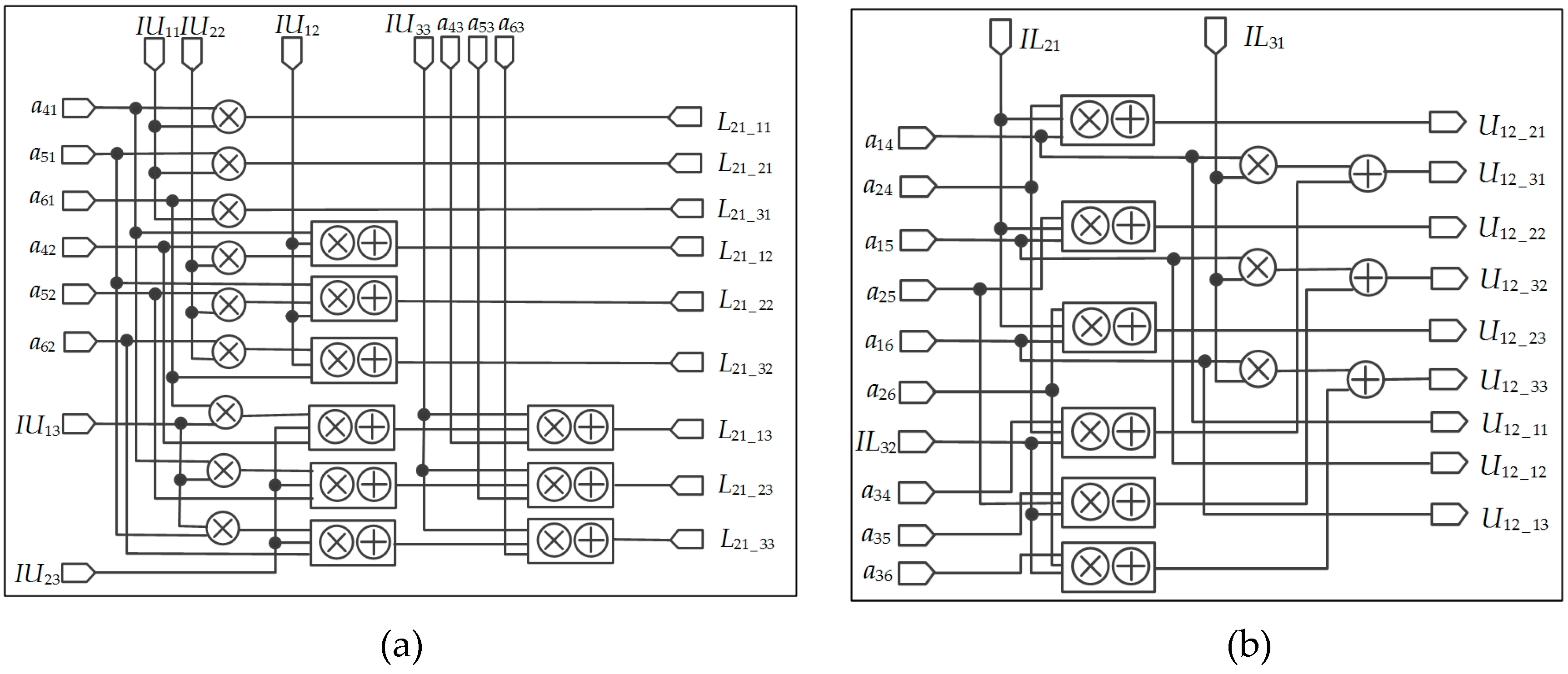
To implement and based on the FPGA, Equations (25) and (26) can be rewritten into Equations (30) and (31). In Equation (30), the elements of the matrix contain three formats, i.e., , , and . In Equation (31), the elements of the matrix contain three formats, i.e., , , and . The proposed parallel architecture for calculation of and is depicted in Figure 9. Twelve multipliers, fifteen MD modules, and three adders are used.
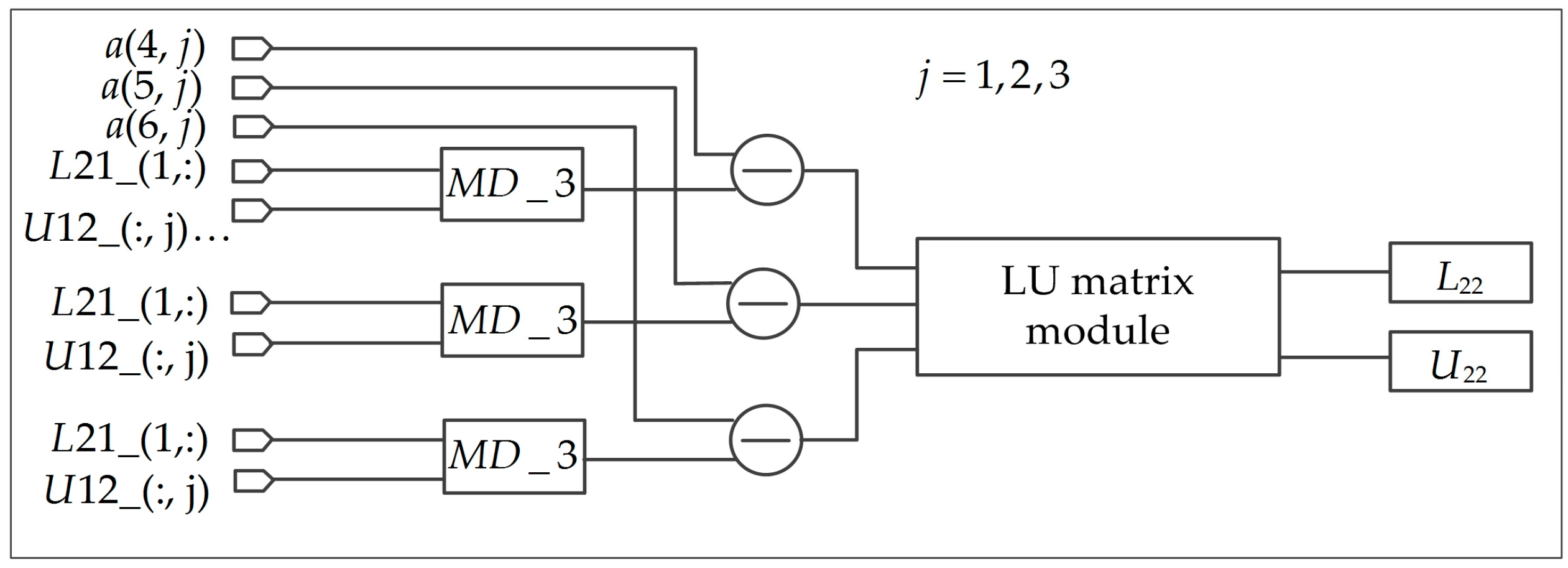
4. FPGA-Based Implementation of and
To implement and , Equation (24) can be described by
where is a matrix, with a similar format of . Therefore, the LU decomposition of is not deduced in details. The parallel implementation is shown in Figure 10.
For the Block LU decomposition, the number of multiplications is about , and division is (where is the dimension of each block, is the size of matrix). In the standard LU decomposition, the number of multiplication operations is about n, and division is [52]. The multipliers and dividers based block LU decomposition are approximately reduced 1.02 and 1.25 times than that the traditional LU decomposition.
3.1.3. FPGA-Based Implantation of the Matrix
When , , , , , and matrices are solved, the block LU decomposition of matrix has been completed,. The processing of inversion matrix is based on the Equation (33).
where and .
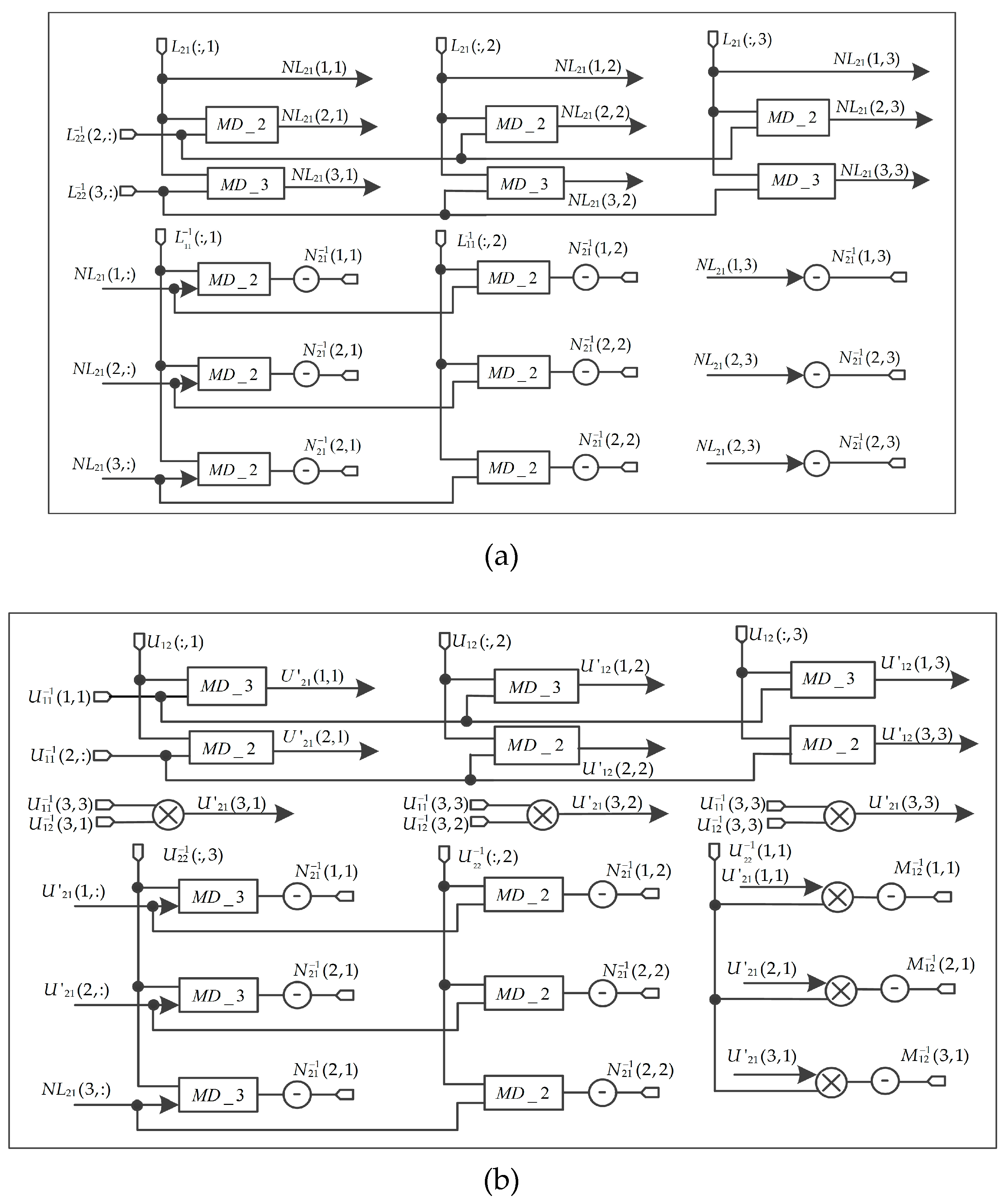
1. FPGA-Based Implementation of and
Figure 11 shows the implementation of and , It contains MD_3 module, MD_2 module and negative operation.
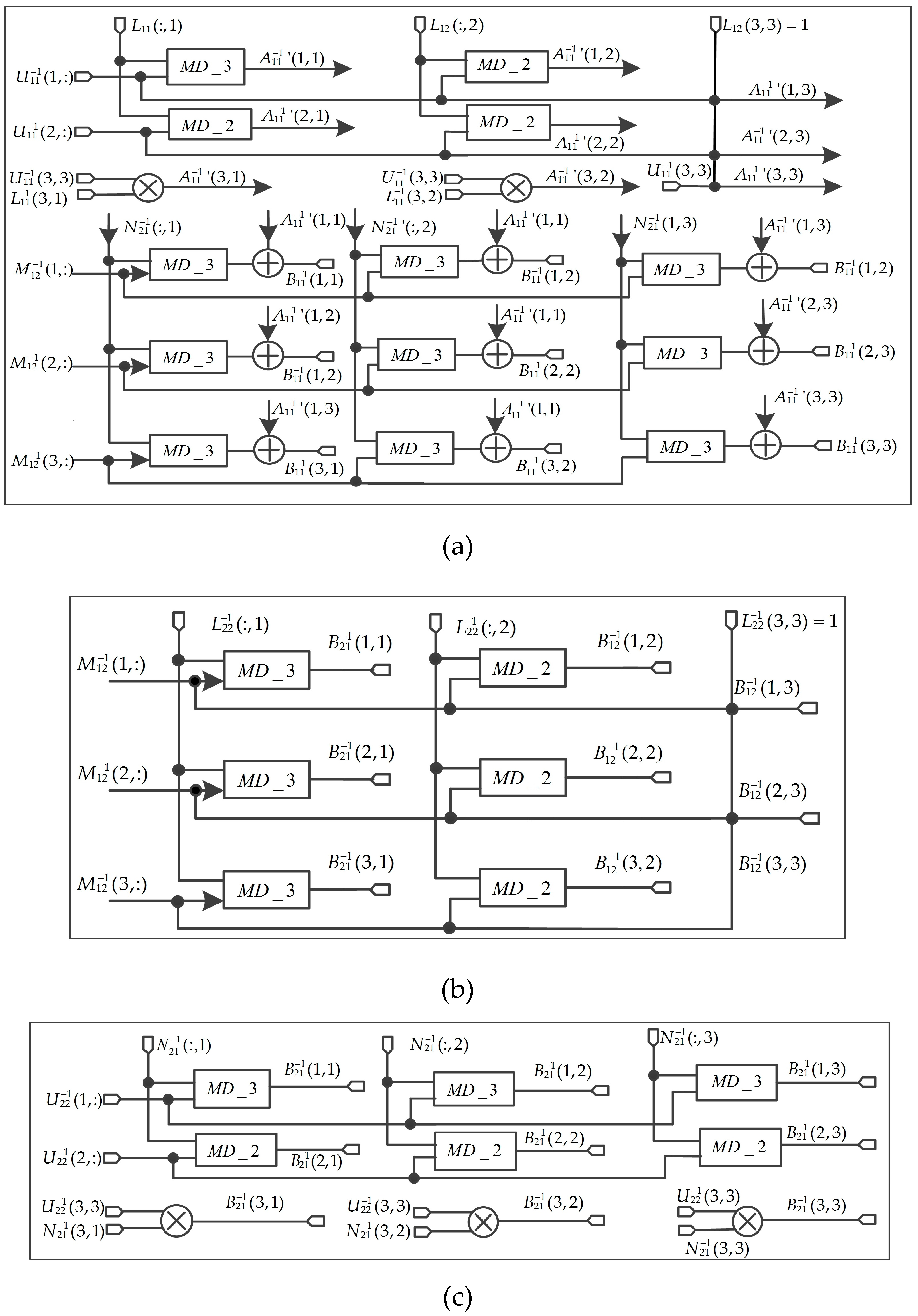
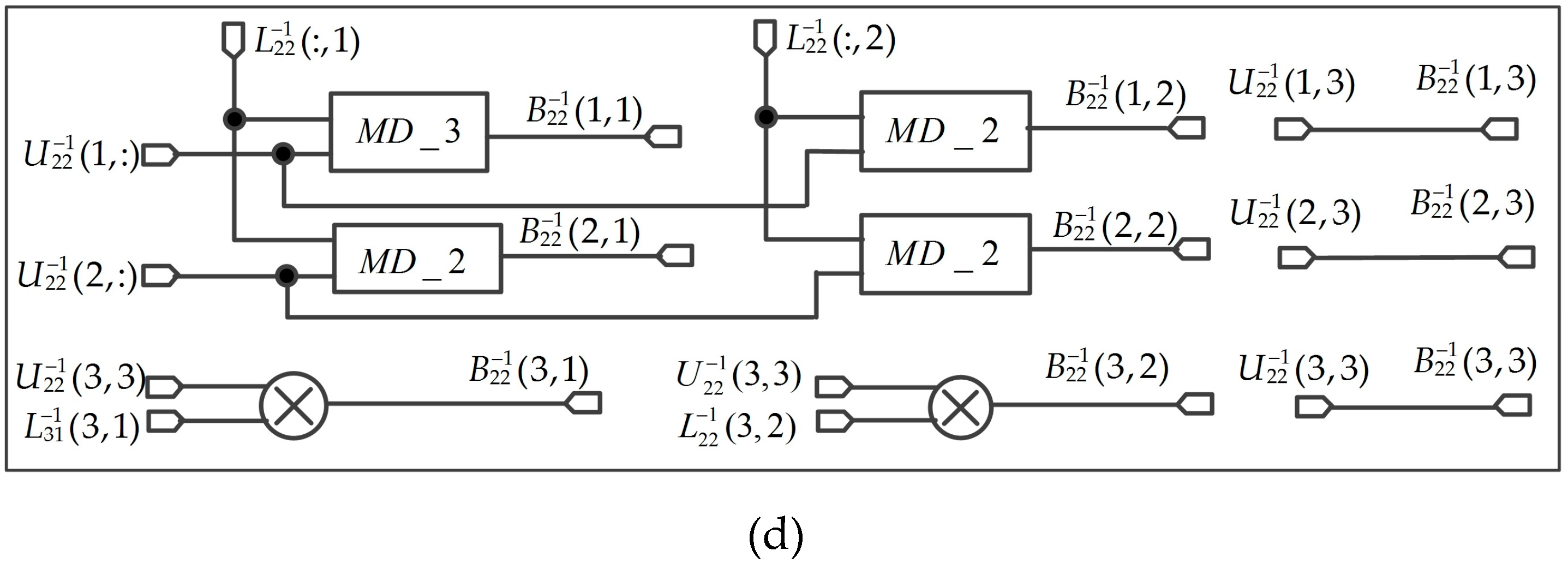
2. FPGA-Based Implementation of
The scheme for is shown in Figure 12. Figure 12a is an FPGA implementation of solving the matrix. Ten MD_3 modules, three MD_2 modules, two multipliers, and nine adders are used to solve the matrix. Figure 12b shows the parallel computation for matrix, three MD_3 modules, and three MD_2 modules are used. The structure for solving the matrix is shown in Figure 12c, three MD_3 modules, three MD_2 modules, and three multipliers are used. Figure 12d shows the implementation of the matrix, one MD_3 module, two MD_2 modules, and two multipliers are used. The Figure 12a through Figure 12d are parallel calculated. Finally, matrix is obtained and the elements are outputted at the same clock cycle.
3.1.4. FPGA-Based Implementation of a and b Matrices
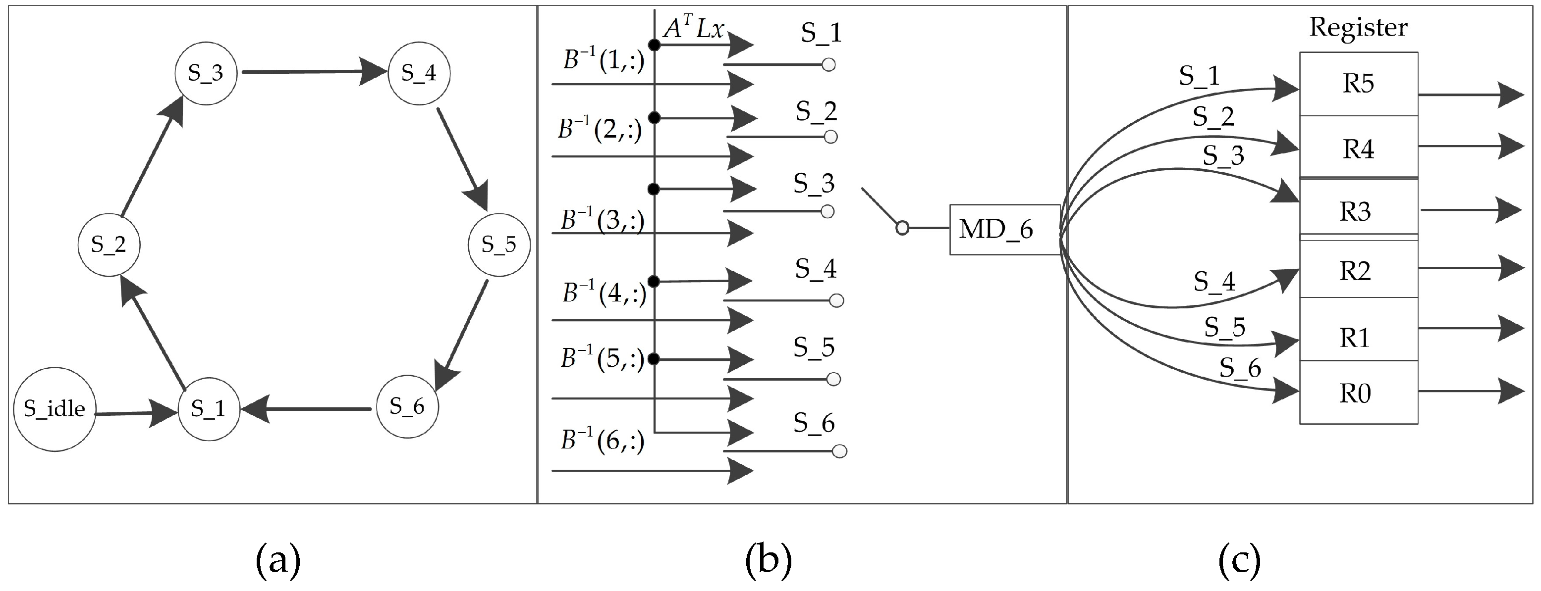
From the ten GCPs data, and matrix can be obtained, since and matrices have the same structure, such as , , , and , the implementation of is given to illustrate the processes. From Equation (34), six MD_10 modules are adopted. Six MD_6 modules are needed for solving Equation (35). Considering the limited resources of an FPGA, a serial framework is used to implement , the strategy is depicted in Figure 13 (such as ).
The details of state transition graph (STG) are as follows:
- S_idle, idle state. When the rst signal is low, the system is in the reset state, all registers (R0, R1, ..., R5) and other signals are reset.
- S_1 to S_6 are the six different state machines (SMs). Under the different SMs, different row values of the matrix with matrix are calculated in the MD_6 modules. The result of MD_6 is serial saved in the registers R5 to R0. When the six SMs are finished, the values of registers R5 to R0 are parallel outputted to the matrix .
- S_1, the first SM. When the rst signal goes high, the current state enters the first state when the enable signal is being received. The values of matrix and are put into the MD_6 module for multiplication and addition. The result is saved in the register R5.
- S_2, the second SM. When the S_1 state is complete, the current state enters the second state. The values of matrix and begin to calculate multiplication and addition. Then, the result is saved in the register R4.
In this order, when the S_6 SM (final State) is completed, the matrix is derived. Under the same clock cycle, the values of the registers R5 to R0 (–) are parallel outputted. The current state returns to the first state. Additionally, each state should contain a certain delay time. The delay time should include MD_6 module operation time and serial storage time.
3.2. FPGA-Based Implementation of Coordinate Transformation and Bilinear Interpolation Algorithm
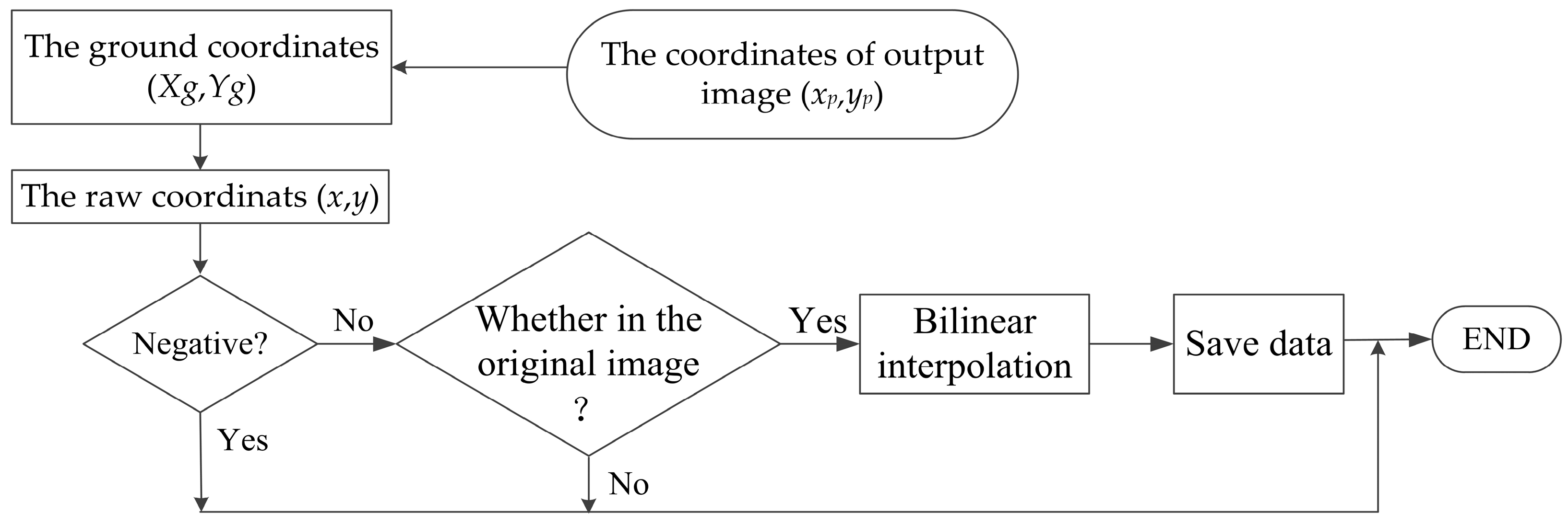
Figure 14 shows the flowchart for the coordinate transformation and bilinear interpolation method, which consists of the transformation from the output image coordinates to the ground coordinates, conversion the ground coordinate to the raw image coordinates, and bilinear interpolation.
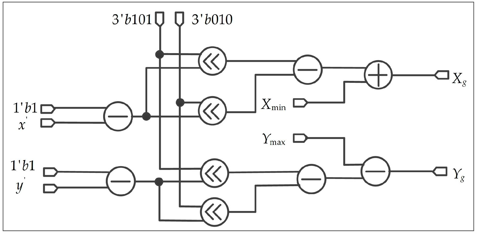
1. FPGA-Based Implementation of and
The purpose of this step is to obtain and in Equation (12) of Section 2.1.2, as shown in Figure 15. In this part, 32-bit integer and shift register are used to reduce the resource utilization of an FPGA. To implement the shift operation, and are approximated as or ( and are integers). For instance, , which can be expressed as the form of . In Figure 15, the symbol “<<” in the circle represents the left shift operation.
2. FPGA-Based Implementation of Bilinear Interpolation
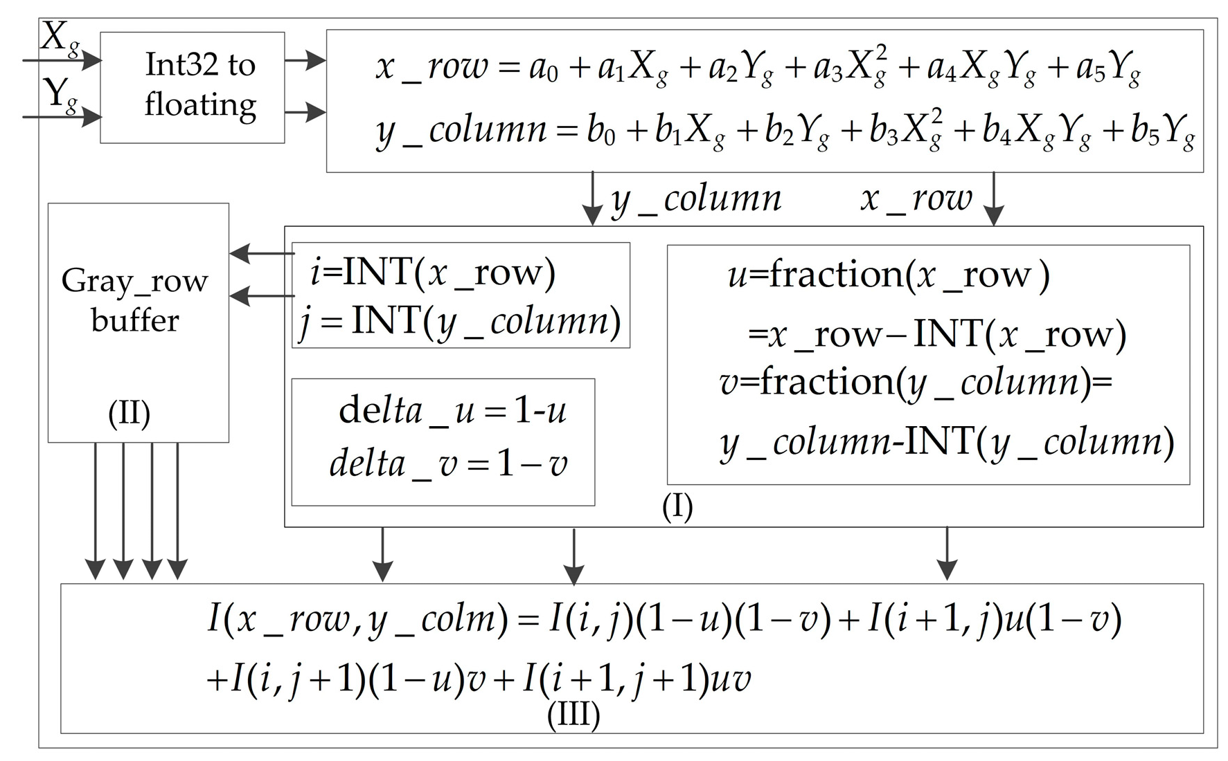
When and are calculated, the coordinates of and are obtained from Equations (14) and (15). The bilinear interpolation algorithm is performed based on the and as shown in Figure 16. As observed from Figure 16, the processing of bilinear interpolation is divided into three steps.
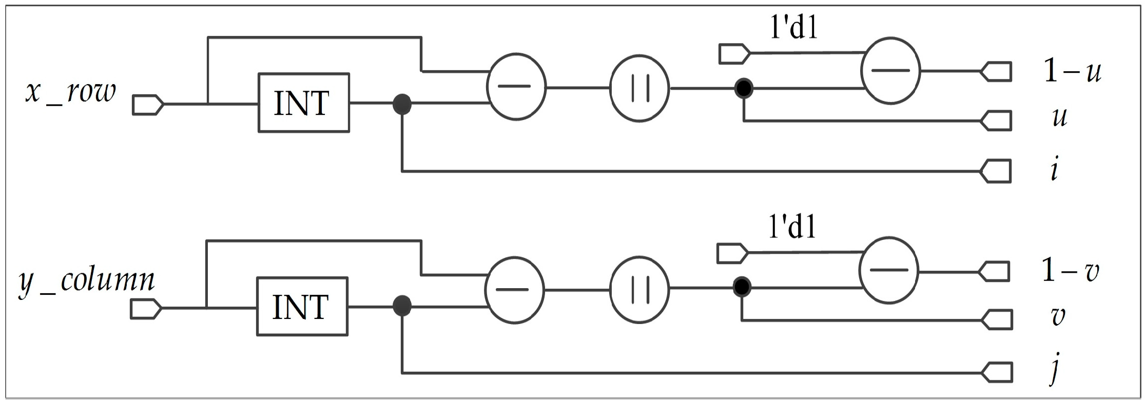
In step (I), the integer part , , the fractional part , and the weight part and of the floating-point coordinates are computed, respectively. Figure 17 shows the parallel implementation method for , , , , and . Four subtractors, two INT (integer) modules and two absolute modules (“||” in the circle) are used.
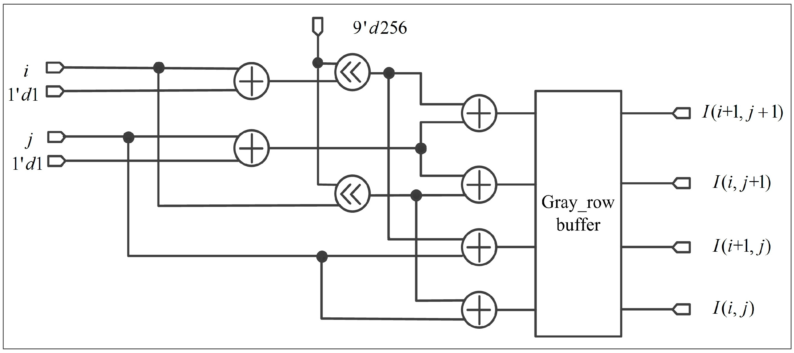
In step (II), it is mainly to calculate the address of four nearest neighbor pixels and read the corresponding gray value. The address of memory can be calculated from Equation (17) of Section 2.2.2. The processing of reading gray value is shown in Figure 18. To reduce the resources of an FPGA, the multiplication is converted into left shift operation.
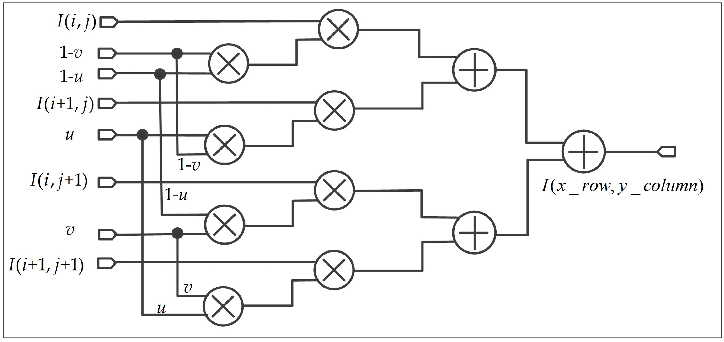
After the values of , , , , , , , , , and are computed, the gray value of the georeferenced image can be calculated in step (III). According to Equation (13) and (16). The implementation of bilinear interpolation algorithm is shown in Figure 19. Eight multipliers and three adders are used to compute the value of .
4. Experiment and Performance Analysis
4.1. The Software and Hardware Environment
The proposed scheme is implemented on a custom-designed board which contains a Xilinx Virtex-7-XC7VX980t-ffg1930-1 FPGA that has 612,000 logic cells, 1,500 kB Block RAM, 1,224,000 Flip-Flops, and 3,600 DSP slices. Additionally, the design tool is Vivado 2014.2, the simulation tool is ModelSim SE-64 10.4, and the hardware design language is Verilog HDL. To validate the proposed method, the georeferenced algorithm is also implemented by MATLAB R2014a, Visual Studio 2015 (C++) and ENVI 5.3 on a PC equipped with an Intel (R) Core i7-4790 CPU @ 3.6 GHz and 8 GB RAM, running Windows 7 (64 bit).
4.2. Data
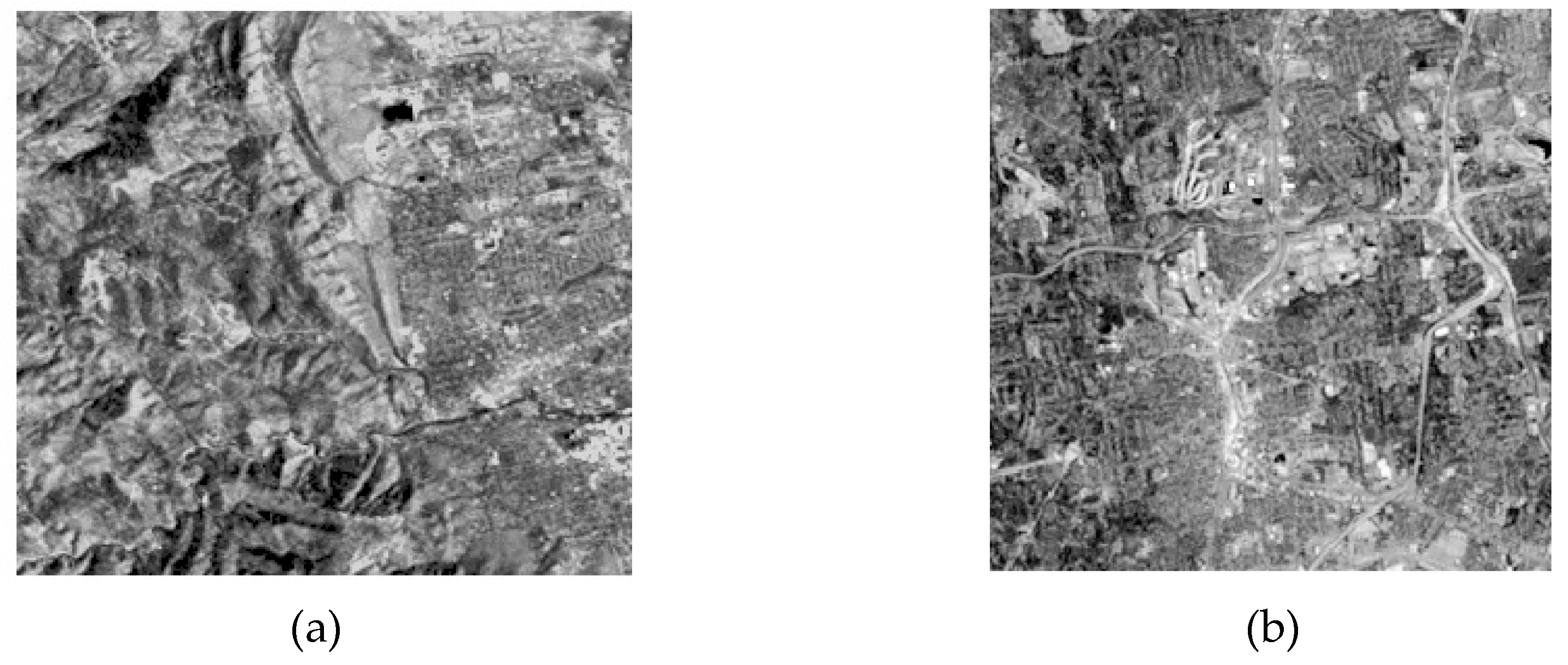
To validate the proposed FPGA-based algorithm, two data sets are used to perform the georeferencing. The first data set is acquired from the ENVI example dataset, i.e., bldt_tm.img and bldt_tm.pts. The second data set is obtained from the ERDAS example dataset, i.e., tmAtlanta.img and panAtanta.img. Figure 20a,b display the raw data sets of bldt_tm.img and tmAtlanta.img, respectively. The image size is 256 × 256 pixels2. The information of two datasets is shown in Table 2.
4.3. Processing Performance
4.3.1. Error Analysis
To quantitatively evaluate the accuracy of the georeferencing implemented using FPGA, the root mean squared error (RMSE) is used in Equation (36) through Equation (38) [45].
where and are coordinates of the georeferenced image which are computed by the proposed method; and are reference geodetic coordinates; and is the number of check points (CPs).
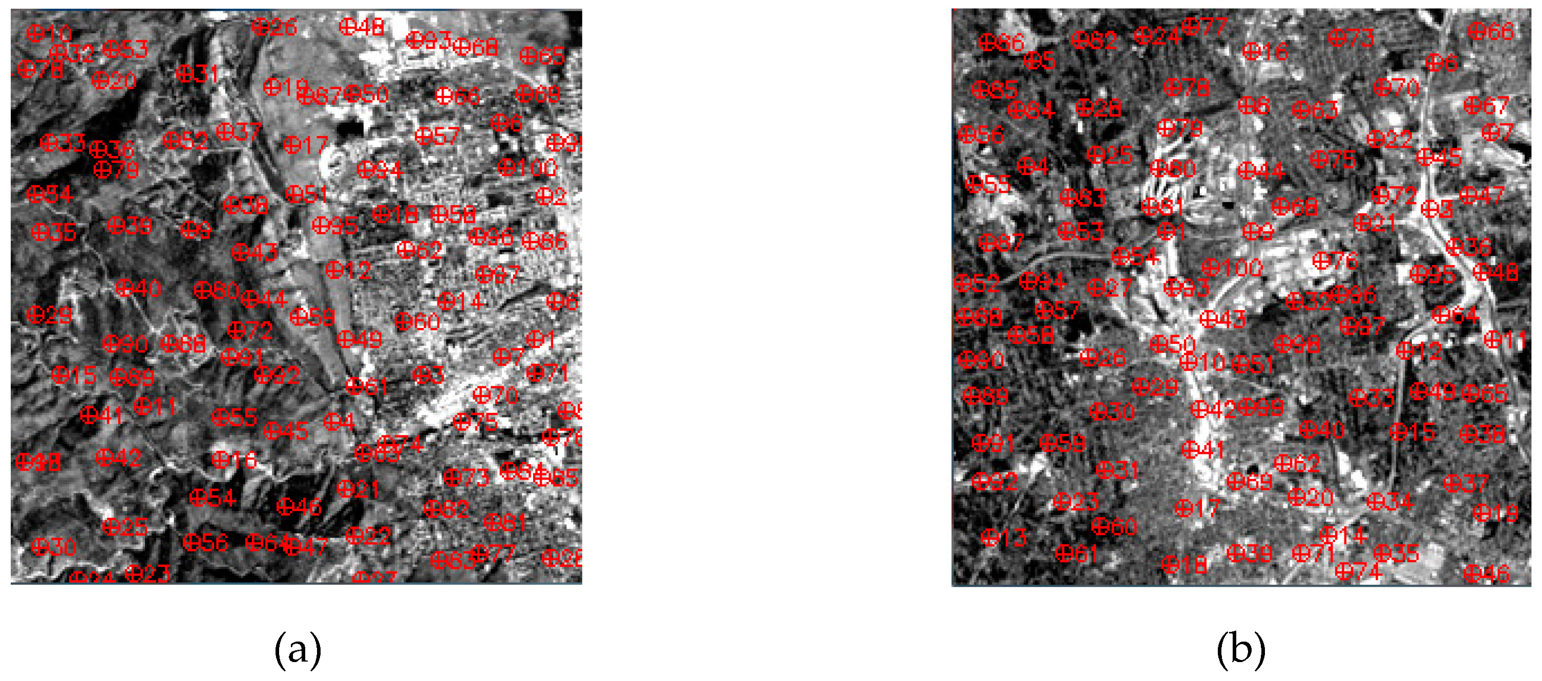
To compute the root mean squared errors (RMSEs), one hundred CPs are selected as shown in Figure 21.
With the experimental results, a few conclusions can be drawn as follows.
(1) From Equation (36) through (38), the RMSEs are computed based on FPGA, MATLAB, Visual Studio (C++), and ENVI, as shown in Table 3. It can be concluded that the RMSEx, RMSEy, and RMSE of the georeferenced image of the first data set implemented using FPGA are 0.1441, 0.1672, and 0.2207 pixels, respectively. The accuracy of the georeferenced using FPGA has the same values when implemented by MATLAB and Visual studio (C++), and is close to the values implemented using ENVI software. Additionally, other statistics, such as maximum, minimum and mean error are computed and listed in Table 4. It can be found that the proposed FPGA-based algorithm has a mean error of x and y coordinates at 0.0775 pixels and 0.0945 pixels, respectively; the minimum and the maximum errors of the x and y coordinates are 0.0008 and 0.0026 pixels, and 0.5113 and 0.4038 pixels, respectively. The accuracy of the various errors are calculated by the proposed algorithm has the same values than those based on MATLAB and Visual Studio (C++), and has a close accuracy than that based on ENVI software.
(2) Table 5 lists the RMSEs of the georeferenced image of the second data set. The values of the RMSEx, RMSEy, and RMSE implemented by FPGA are 0.0965, 0.1268, and 0.1593 pixels, respectively. The RMSEs implemented using FPGA have the same accuracy than those based on MATLAB and Visual Studio (C++), and have a close accuracy implemented using ENVI software. However, it can be considered acceptable for the absolute error is less than one pixel [53]. In addition, maximum, minimum and mean errors are computed and listed in Table 6. It can be found that the mean errors implemented using FPGA of the x and y coordinates are 0.0789 and 0.1144 pixels, respectively, and the minimum and maximum errors for the x and y coordinates are 0.0008 and 0.0046 pixels, and 0.2613 and 0.2081 pixels, respectively.
4.3.2. Gray Value Comparison
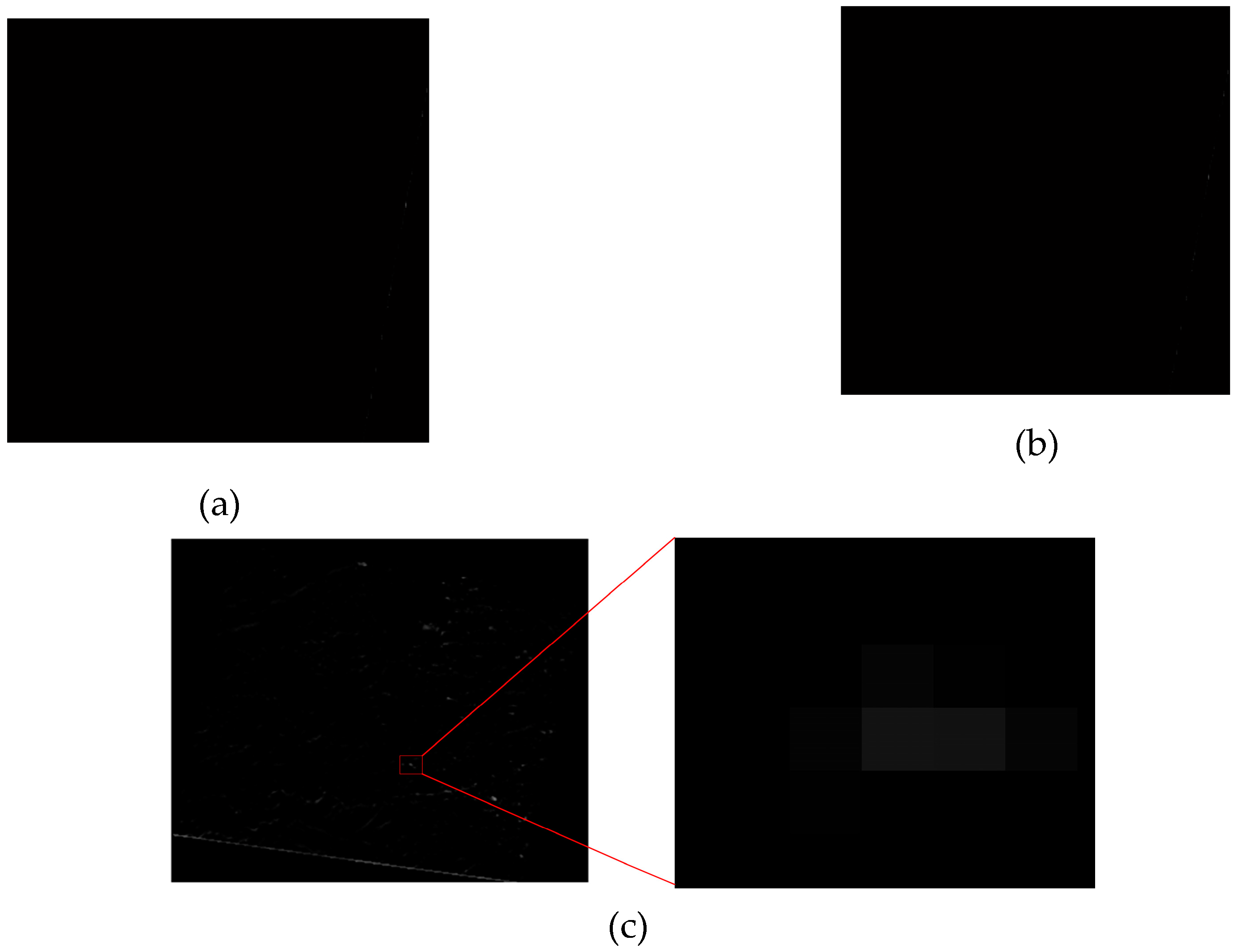
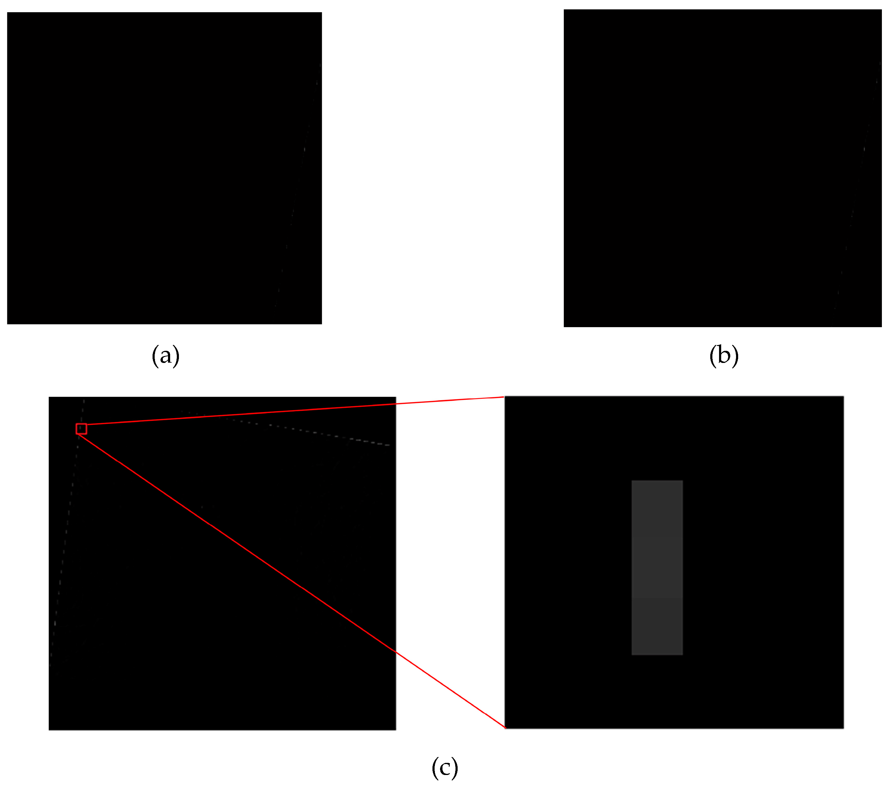
To verify the accuracy of gray value, the gray levels of georeferenced image are compared to those implemented using FPGA, MATLAB, Visual Studio (C++), and ENVI software. The georeferenced image implemented using FPGA as a referencing image, called “Ref-Img”. The georeferenced image implemented using MATLAB, Visual Studio (C++), and ENVI are called “Img-MATLAB”, “Img-C++”, and “Img-ENVI”, respectively. The gray differences between the Ref-Img and those georeferenced images implemented by MATLAB, Visual Studio (C++), and ENVI are obtained and shown in Figure 24 and Figure 25.
As observed from Figure 24, the gray values of Figure 24a,b are 0, which means the proposed method implemented using FPGA has the same accuracy with the implemented by MATLAB, and Visual Studio (C++) [55,56]. Figure 24c indicates that the difference image between Ref-Img and Img-ENVI has many pixels are not same. The mean values of Figure 24a–c are 0, 0, and 0.713 respectively, which are less than 1 pixel.
As observe from Figure 25, the proposed method has the same accuracy as those implemented using MATLAB, and Visual Studio (C++), and has a small portion of the gray values are different from the Img-ENVI. The mean values of the Figure 25a–c are 0, 0, and 0.1265, respectively, which are all less than 1 pixel.
4.3.3. Resource Occupation Analysis
The resource utilization ration, including the flip-flop (FF), look-up-table (LUT) and DSP48s of the FPGA for the coordinate transformation method and bilinear interpolation function are assessed, respectively.
In the coordinate transformation method, 250,656 LUTs, 499,268 registers, and 388 DSP48s are utilized at rates of 40.96% (250656/612000 = 40.96%), 40.79%, and 37.96%, respectively (see Table 7).
In the bilinear interpolation function, floating-point and 32-bit fixed-point mixed operations are adopted, which can reduce the resource consumption of an FPGA. Table 8 lists the resources occupied for the bilinear interpolation scheme. 27,218 LUTs, 45,823 registers, 456 RAM/FIFO, and 267 DSP48s are utilized at rates of 4.45%, 3.74%, 30.40%, and 7.42%, respectively.
4.3.4. Processing Speed Comparison
The processing speed is considered as one of the most important factors for implementation by an FPGA. Table 9 lists the processing speed implemented by FPGA, Visual Studio (C++) and MATLAB. The size of the first raw image is 256 × 256 pixels2. After georeferencing, the size of georeferenced image is 281 × 281 pixels2. The running time of the georeferencing method for the first image using FPGA, Visual Studio (C++) and MATLAB is 0.13s, 1.06s, and 1.12s, respectively. The size of the second raw image is 256 × 256 pixels2; after georeferencing, the image size is 285 × 277 pixels2. The running time of the georeferencing method for the second raw image using FPGA, Visual Studio (C++) and MATLAB is 0.15s, 1.21s, 1.26s, respectively. To put it simply, the processing speed using FPGA is 8 times faster than that based on PC computer.
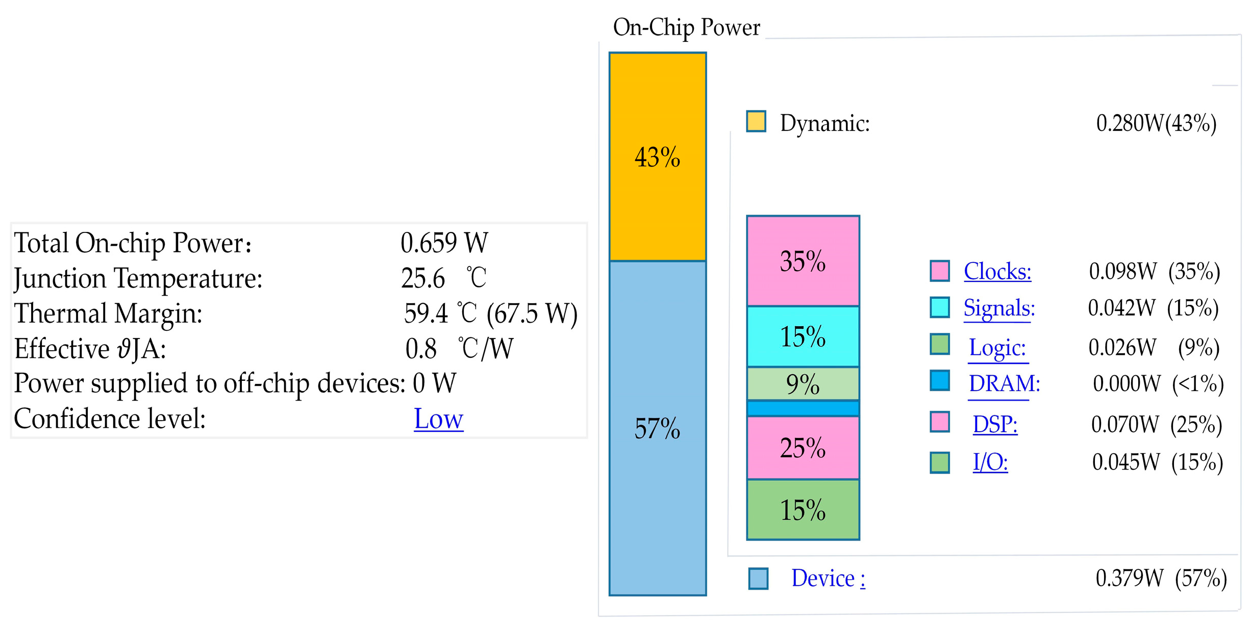
4.3.5. Power Consumption
With the development of technology and the improvement of system performance, low power consumption has become one of the measurement objectives of on-board system. Resources, speed, and power consumption are three key factors in FPGA design. To obtain the power consumption, Vivado software provides a comprehensive methodologies and strategies for power consumption As observed from Figure 26, the powers of the dynamic and the device are 0.280 W (43%) and 0.379 W (57%), respectively. The total on-chip power is 0.659 W, which is acceptable in on-board processing platform.
5. Conclusions
This paper presents a novel scheme for on-board georeferencing using FPGA optimized second-order polynomial equation and bilinear interpolation scheme, which consists of five modules: input data, coordinate transformation, bilinear interpolation and output data. The main contributions of this paper are as follows.
First, a comprehensive framework has been developed to optimize the georeferencing algorithm based on an FPGA. (1) A floating-point block LU decomposition is used to inverse the matrix. Compared with the traditional LU decomposition, the multiplication and division operations are reduced by 1.02 and 1.25 times, respectively. The block LU decomposition method can reduce the complexity for inverting matrix and speed up the operation. (2) To reduce resource consumption of an FPGA, some strategies are adopted in programming, i.e., 32-bit integer and floating-point mixed operation and serial-parallel data communication.
Second, the performances of the proposed algorithm are evaluated by error analysis, gray value comparison, resource occupation analysis, processing speed comparison, and power consumption. The RMSEs are less than one pixel, and other statistics, such as maximum, minimum, and mean error are less than one pixel. The gray values of the georeferenced image when implemented using the FPGA have the same accuracy as those implemented using MATLAB and Visual Studio (C++), and have a very close accuracy implemented using ENVI software. The processing speed using the proposed algorithm is 8 times faster than that based on PC computer. The on-chip power consumption is 0.659 W.
Therefore, it can be concluded that the proposed georeferencing algorithm implemented using FPGA with second-order polynomial model and bilinear interpolation algorithm can achieve real-time geographic referencing for remote sensing images.
Author Contributions
G.Z. conceives and designs the experiments; D.L. performs the experiments and writes the paper; J.H. offers the help of FPGA implementation; L.S. analyzes the data; R.Z. and X.Z. revise the manuscript. X.C. improves the English language and style.
Funding
This work was supported by grants from the Natural Science Foundation of China (grant No. 41431179, 41601365); GuangXi Key Laboratory for Spatial Information and Geomatics Program (Contract No.17-259-16-09); GuangXi innovative Development Grand under Grant 2018AA13005; GuangXi Key Research and development Program of China under Grant number 2016YFB502501; GuangXi innovative Development Grand Grant, (the grant number: GuiKe AA18118038). The State Oceanic Administration under Grant number [2014]#58; GuangXi Natural Science Foundation under grant number 2015GXNSFDA139032; and Guangxi Key Laboratory of Spatial Information and Geomatics Program under grant numbers 15-140-07-01 and 16-380-25-12.
Acknowledgments
The author would like to thank the reviewers for their constructive comments and suggestions.
Conflicts of Interest
The authors declare no conflict of interest.
References
- Joyce, K.E.; Belliss, S.E.; Samsonov, S.V.; Mcneill, S.J.; Glassey, P.J. A review of the status of satellite remote sensing and image processing techniques for mapping natural hazards and disasters. Prog. Phys. Geogr. 2009, 33, 183–207. [Google Scholar] [CrossRef]
- Tralli, D.M.; Blom, R.G.; Zlotnicki, V.; Donnella, A.; Evans, D.L. Satellite remote sensing of earthquake, volcano, flood, landslide and coastal inundation hazards. J. Photogr. Remote Sens. 2005, 59, 185–198. [Google Scholar] [CrossRef]
- Sanyal, J.; Lu, X.X. Application of remote sensing in flood management with special reference to monsoon Asia: A review. Nat. Hazards 2004, 33, 283–301. [Google Scholar] [CrossRef]
- Zhou, G. Near real-time orthorectificatoin and nosaic of small UAV-based video flow for time-critical event response. IEEE Trans. Geosci. Remote Sens. 2009, 47, 739–747. [Google Scholar] [CrossRef]
- Zhou, G.; Zhang, R.; Liu, N.; Huang, J.; Zhou, X. On-board ortho-rectification for images based on an FPGA. Remote Sens. 2017, 9, 874. [Google Scholar] [CrossRef]
- González, G.; Bernabé, S.; Mozos, D.; Plaza, A. FPGA Implementation of an algorithm for automatically detecting targets in remotely Sensed hyperspectral images. IEEE J. Sel. Top. Appl. Earth Obs. Remote Sens. 2016, 9, 4334–4343. [Google Scholar] [CrossRef]
- Qi, B.; Shi, H.; Zhuang, Y.; Chen, H.; Chen, L. On-board, real-time preprocessing system for optical remote-sensing imagery. Sensors 2018, 18, 1328. [Google Scholar] [CrossRef] [PubMed]
- Dawood, A.S.; Visser, S.J.; Williams, J.A. Reconfigurable FPGAs for real time image processing in space. In Proceedings of the 2002 14th International Conference on Digital Signal Processing Proceedings, DSP 2002 (Cat. No. 02TH8628), Santorini, Greece, 1–3 July 2002; pp. 845–848. [Google Scholar]
- Zhang, Y.; Kerle, N. Satellite remote sensing for near-real time data collection. In Geospatial Information Technology for Emergency Response; CRC Press: Taylor & Francis, London, UK, 2008; pp. 91–118. [Google Scholar]
- Zhou, G.; Chen, W.; Kelmelis, J.A.; Zhang, D. A comprehensive study on urban true orthorectification. IEEE Trans. Geosci. Remote Sens. 2005, 43, 2138–2147. [Google Scholar] [CrossRef]
- Zhou, G. Geo-Referencing of video flow from small low-cost civilian UAV. IEEE Trans. Autom. Eng. Sci. 2010, 7, 156–166. [Google Scholar] [CrossRef]
- Ziboon, A.R.T.; Mohammed, I.H. Accuracy assessment of 2D and 3D geometric correction models for different topography in Iraq. Eng. Technol. J. Part A Eng. 2013, 31, 2076–2085. [Google Scholar]
- Kartal, H.; Sertel, E.; Alganci, U. Comperative analysis of different geometric correction methods for very high resolution pleiades images. In Proceedings of the 2017 8th International Conference on Recent Advances in Space Technologies (RAST), Istanbul, Turkey, 19–22 June 2017; pp. 171–175. [Google Scholar]
- Wang, T.; Zhang, G.; Li, D.; Tang, X.; Pan, H.; Zhu, X.; Chen, C. Geometric accuracy validation for ZY-3 satellite imagery. IEEE Geosci. Remote Sens. Lett. 2014, 11, 1168–1171. [Google Scholar] [CrossRef]
- Chen, J.; Joang, T.; Lu, W.; Han, M. The geometric correction and accuracy assessment based on Cartosat-1 satellite image. In Proceedings of the 2010 3rd International Congress on Image and Signal Processing, Yantai, China, 16–18 October 2010; pp. 1253–1257. [Google Scholar]
- Lee, C.A.; Gasster, S.D.; Plaza, A.; Chang, C.I.; Huang, B. Recent developments in high performance computing for remote sensing: A review. IEEE J. Sel. Top. Appl. Earth Obs. Remote Sens. 2011, 4, 508–527. [Google Scholar] [CrossRef]
- Plaza, A.; Valencia, D.; Plaza, J.; Martinez, P. Commodity cluster-based parallel processing of hyperspectral imagery. J. Parallel Distrib. Comput. 2006, 66, 345–358. [Google Scholar] [CrossRef]
- Plaza, A.; Du, Q.; Chang, Y.L.; King, R.L. High performance computing for hyperspectral remote sensing. IEEE J. Sel. Top. Appl. Earth Obs. Remote Sens. 2011, 4, 528–544. [Google Scholar] [CrossRef]
- Fang, L.; Wang, M.; Li, D.; Pan, J. CPU/GPU near real-time preprocessing for ZY-3 satellite images: Relative radiometric correction, MTF compensation, and geocorrection. ISPRS J. Photogr. Remote Sens. 2014, 87, 229–240. [Google Scholar] [CrossRef]
- Van der Jeught, S.; Buytaert, J.A.N.; Dirckx, J.J. Real-time geometric lens distortion correction using a graphics processing unit. Opt. Eng. 2012, 51. [Google Scholar] [CrossRef]
- Thomas, O.; Trym, V.H.; Ingebrigt, W.; Ingebrigt, W. Real-time georeferencing for an airborne hyperspectral imaging system. Algorithms Technol. Multispectral Hyperspectral Ultraspectral Imagery XVII 2011, 8048. [Google Scholar] [CrossRef]
- Reguera-Salgado, J.; Calvino-Cancela, M.; Martin-Herrero, J. GPU geocorrection for airborne pushbroom imagers. IEEE Trans. Geosci. Remote Sens. 2012, 50, 4409–4419. [Google Scholar] [CrossRef]
- López-Fandiño, J.; Barrius, P.Q.; Heras, D.B.; Argüello, F. Efficient ELM-based techniques for the classification of hyperspectral remote sensing images on Commodity GPUs. IEEE J. Sel. Top. Appl. Earth Obs. Remote Sens. 2015, 8, 2884–2893. [Google Scholar] [CrossRef]
- Lu, J.; Zhang, B.; Gong, Z.; Li, E.; Liu, H. The remote-sensing image fusion based on GPU. In Proceedings of the International Archives of the Photogrammetry, Remote Sensing and Spatial Information Sciences, Beijing, China, 23 October 2008; pp. 1233–1238. [Google Scholar]
- Zhu, H.; Cao, Y.; Zhou, Z.; Gong, M. Parallel multi-temporal remote sensing image change detection on GPU. In Proceedings of the IEEE International Parallel and Distributed Processing Symposium Workshops & PhD Forum, IEEE Computer Society, Shanghai, China, 21–25 May 2012; pp. 1898–1904. [Google Scholar]
- Ma, Y.; Chen, L.; Liu, P.; Lu, K. Parallel programing templates for remote sensing image processing on GPU architectures: Design and implementation. Computing 2016, 98, 7–33. [Google Scholar] [CrossRef]
- Lopez, S.; Vladimirova, T.; Gonzalez, G.; Resano, J.; Mozos, D. The promise of reconfigurable romputing for hyperspectral imaging onboard systems: A review and trends. Proc. IEEE 2013, 101, 698–722. [Google Scholar] [CrossRef]
- Zhou, G.; Baysal, O.; Kaye, J.; Habib, S.; Wang, C. Concept design of future intelligent earth observing satellites. Int. J. Remote Sens. 2004, 25, 2667–2685. [Google Scholar] [CrossRef]
- Huang, J.; Zhou, G.; Zhang, D.; Zhang, G.; Zhang, R.; Baysal, O. An FPGA-based implementation of corner detection and matching with outlier rejection. Int. J. Remote Sens. 2018, 1–20. [Google Scholar] [CrossRef]
- Pakartipangi, W.; Darlis, D.; Syihabuddin, B.; Wijanto, H. Analysis of camera array on board data handling using FPGA for nano-satellite application. In Proceedings of the International Conference on Telecommunication Systems Services and Applications, Bandung, Indonesia, 25–26 November 2015; pp. 1–6. [Google Scholar]
- Huang, J.; Zhou, G.; Zhou, X. A new FPGA architecture of fast and brief algorithm for on-board corner detection and matching. Sensors 2018, 18, 1014. [Google Scholar] [CrossRef] [PubMed]
- Yu, G.; Vladimirova, T.; Sweeting, M.N. Image compression systems on board satellites. Acta Astronautica 2009, 64, 988–1005. [Google Scholar] [CrossRef]
- Long, T.; Jiao, W.; He, G.; Zhang, Z. A fast and reliable matching method for automated georeferencing of remotely-sensed imagery. Remote Sens. 2016, 8, 56. [Google Scholar] [CrossRef]
- Williams, J.A.; Dawood, A.S.; Visser, S.J. FPGA-based cloud detection for real-time onboard remote sensing. In Proceedings of the 2002 IEEE International Conference on Field-Programmable Technology (FPT), Hong Kong, China, 16–18 December 2002; pp. 110–116. [Google Scholar]
- González, C.; Mozos, D.; Resano, J.; Plaza, A. FPGA implementation of the N-FINDR algorithm for remotely sensed hyperspectral image analysis. IEEE Trans. Geosci. Remote Sens. 2012, 50, 374–388. [Google Scholar] [CrossRef]
- Swann, R.; Hawkins, D.; Westwellroper, A.; Johnstone, W. The potential for automated mapping from geocoded digital image data. Photogr. Eng. Remote Sens. 1988, 54, 187–193. [Google Scholar]
- Savoy, F.M.; Dev, S.; Lee, Y.H.; Winkler, S. Geo-referencing and stereo calibration of ground-based Whole Sky Imagers using the sun trajectory. In Proceedings of the 2016 IEEE International Geoscience and Remote Sensing Symposium (IGARSS), Beijing, China, 10–15 July 2016; pp. 7473–7476. [Google Scholar]
- Jensen, J.R.; Lulla, K. Introductory Digital image processing-A remote sensing perspective. Environ. Eng. Geosci. 2007, 13, 89–90. [Google Scholar] [CrossRef]
- Chen, L.C.; Teo, T.A.; Liu, C.L. The geometrical comparisons of RSM and RFM for FORMOSAT-2 satellite images. Photogr. Eng. Remote Sens. 2006, 72, 573–579. [Google Scholar] [CrossRef]
- Bannari, A.; Morin, D.; Bénié, G.B.; Bonn, F.J. A theoretical review of different mathematical models of geometric corrections applied to remote sensing images. Remote Sens. Rev. 1995, 13, 27–47. [Google Scholar] [CrossRef]
- Toutin, T. Geometric processing of remote sensing images: Models, algorithms and methods. Int. J. Remote Sens. 2004, 25, 1893–1924. [Google Scholar] [CrossRef]
- Raffa, M.; Mercogliano, P.; Galdi, C. Georeferencing raster maps using vector data: A meteorological application. In Proceedings of the 2016 IEEE Metrology for Aerospace (MetroAeroSpace), Florence, Italy, 22–23 June 2016; pp. 102–107. [Google Scholar]
- Zhou, G.; Ron, L. Accuracy evaluation of ground points from IKONOS high-resolution satellite imagery. Photogr. Eng. Remote Sens. 2000, 66, 1103–1112. [Google Scholar]
- Zhou, G.; Yue, T.; Shi, Y.; Zhang, R.; Huang, J. Second-order polynomial equation-based block adjustment for orthorectification of DISP imagery. Remote Sens. 2016, 8, 680. [Google Scholar] [CrossRef]
- Shlien, S. Geometric correction, registration, and resampling of Landsat imagery. Can. J. Remote Sens. 1979, 5, 74–89. [Google Scholar] [CrossRef]
- Gribbon, K.T.; Bailey, D.G. A novel approach to real-time bilinear interpolation. In Proceedings of the DELTA 2004 Second IEEE International Workshop on Electronic Design, Test and Applications, Perth, WA, Australia, 28–30 January 2004; pp. 126–131. [Google Scholar]
- Bailey, D.G. Design for Embedded Image Processing on FPGAs; John Wiley & Sons (Asia) Pte Ltd.: solaris south tower, Singapore, 2011; pp. 275–305. ISBN 978-0-470-82849-6. [Google Scholar]
- Huang, J. FPGA-Based Optimization and Hardware Implementation of P-H Method for Satellite Relative Attitude and Absolute Attitude Solution. Ph.D. Thesis, Tianjin University, Tianjin, China, 2019. [Google Scholar]
- Zhou, G.; Huang, J.; Shu, L. An FPGA-based P-H method on-board solution for satellite relative altitude. Geomat. Inf. Sci. Wuhan University. 2018, 43, 1–9. [Google Scholar] [CrossRef]
- Daga, V.; Govindu, G.; Prasanna, V.; Gangadharapalli, S.; Sridhar, V. Efficient floating-point based block LU decomposition on FPGAs. In Proceedings of the International Conference on Engineering of Reconfigurable Systems and Algorithms (Ersa’04), Las Vegas, NV, USA, 21–24 June 2004; pp. 276–279. [Google Scholar]
- Gill, T.; Collett, L.; Armston, J.; Eustace, A.; Danaher, T.; Scarth, P.; Flood, N.; Phinn, S. Geometric correction and accuracy assessment of landsat-7 etm+ and landsat-5 tm imagery used for vegetation cover monitoring in queensland, Australia from 1988 to 2007. Surveyor 2010, 55, 273–287. [Google Scholar] [CrossRef]
- Chen, J.; Ji, K.; Shi, Z.; Liu, W. Implementation of block algorithm for LU factorization. In Proceedings of the 2009 WRI World Congress on Computer Science and Information Engineering, Los Angeles, CA, USA, 31 March–2 April 2009; pp. 569–573. [Google Scholar]
- Richards, J.A.; Richards, J.A. Remote Sensing Digital Image Analysis; Springer: Berlin/Heidelberg, Germany, 1999; pp. 39–74. ISBN 978-3-642-30062-2. [Google Scholar]
- Schowengerdt, R.A. Chapter 7-correction and calibration. In Remote Sensing, 3rd ed.; Academic Press: Cambridgem, MA, USA, 2007; p. 285-XXII. ISBN 978-0-12-369407-2. [Google Scholar]
- French, J.C.; Balster, E.J.; Turri, W.F. A 64-bit orthorectification algorithm using fixed-point arithmetic. High-Perform. Comput. Remote Sens. 2013, 8895. [Google Scholar] [CrossRef]
- Shaffer, D.A. An FPGA Implementation of Large-Scale Image Orthorectification. Ph.D. Thesis, University of Dayton, Dayton, OH, USA, 2018. [Google Scholar]
Figure 1.
The georeferenced image size. (a) Input image. (b) Output image. (c) Incorrect output image. :, upper right; :, upper left; :, lower left; :, lower right. is the input image. is the storage area for the georeferenced image. is the georeferenced image.
Figure 1.
The georeferenced image size. (a) Input image. (b) Output image. (c) Incorrect output image. :, upper right; :, upper left; :, lower left; :, lower right. is the input image. is the storage area for the georeferenced image. is the georeferenced image.

Figure 2.
The architecture for the bilinear interpolation. (a) Distributions of the four nearest neighbor pixels and (b) 3D spatial distribution of the bilinear interpolation.
Figure 2.
The architecture for the bilinear interpolation. (a) Distributions of the four nearest neighbor pixels and (b) 3D spatial distribution of the bilinear interpolation.

Figure 3.
Raw image mapping with double data rate (DDR)

Figure 4.
A field programmable gate array (FPGA) architecture for the georeferenced remote sensing images with second-order polynomial equation and bilinear interpolation scheme. RAM: random access memory; clk: clock; rst: reset; en: enable.
Figure 4.
A field programmable gate array (FPGA) architecture for the georeferenced remote sensing images with second-order polynomial equation and bilinear interpolation scheme. RAM: random access memory; clk: clock; rst: reset; en: enable.

Figure 5.
The proposed parallel implementation of the solving coefficient.

Figure 6.
The architectures of .

Figure 7.
Parallel computation block lower-upper (LU) decomposition of .

Figure 8.
The architecture FPFA-based for and matrices. (a) The architecture for solving . (b) The architecture for solving .
Figure 8.
The architecture FPFA-based for and matrices. (a) The architecture for solving . (b) The architecture for solving .

Figure 9.
Parallel computation method for and . (a) The architecture of . (b) The architecture of .

Figure 10.
The architecture of and .

Figure 11.
Implementation of and (a) The architecture of . (b) The architecture of .

Figure 12.
The implementation of . (a) Calculate matrix. (b) Solve matrix. (c) Calculate matrix. (d) Compute matrix.
Figure 12.
The implementation of . (a) Calculate matrix. (b) Solve matrix. (c) Calculate matrix. (d) Compute matrix.


Figure 13.
The processing of state transition graph (STG). (a) The state machine. (b) Serial framework. (c) Serial input and parallel output.
Figure 13.
The processing of state transition graph (STG). (a) The state machine. (b) Serial framework. (c) Serial input and parallel output.

Figure 14.
The flowchart of the coordinate transformation and bilinear interpolation.

Figure 15.
Parallel computation method for and .

Figure 16.
The diagram of bilinear interpolation.

Figure 17.
The parallel implementation method for , , , , and .

Figure 18.
The architecture for parallel reading gray values.

Figure 19.
The parallel computation for bilinear interpolation.

Figure 20.
The raw image. (a) The first raw image. (b) The second raw image.

Figure 21.
Check points distribution in: (a) the first image and (b) the second image.

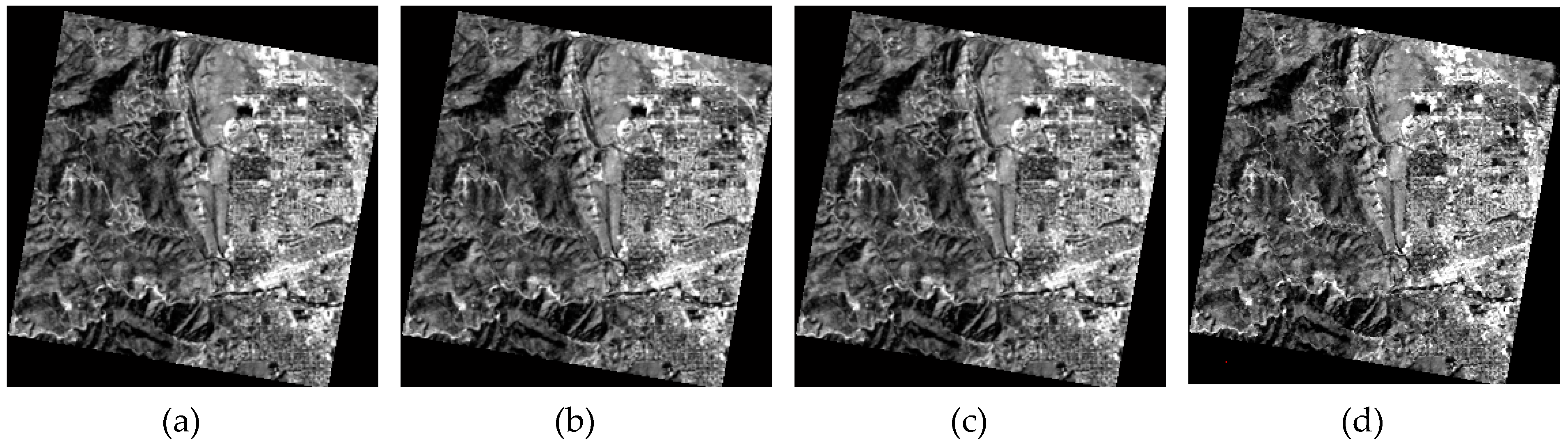
Figure 22.
The georeferenced image of the first data set. (a) By FPGA. (b) By MATLAB. (c) By Visual Studio (C++). (d) By ENVI 5.3.
Figure 22.
The georeferenced image of the first data set. (a) By FPGA. (b) By MATLAB. (c) By Visual Studio (C++). (d) By ENVI 5.3.

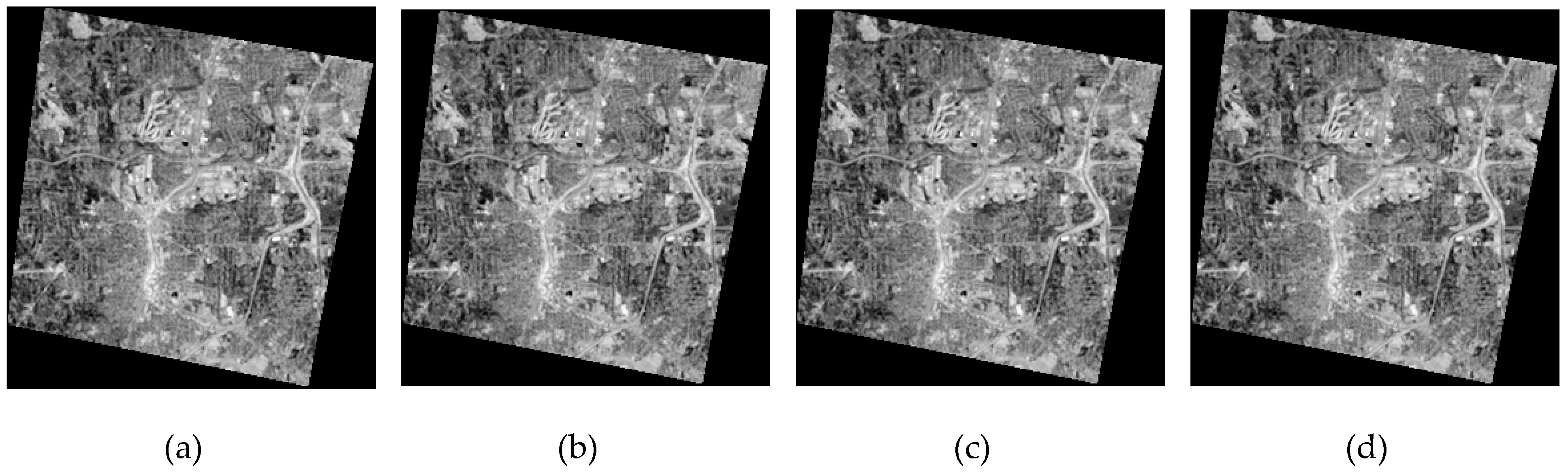
Figure 23.
The georeferenced image of the second data set. (a) By FPGA. (b) By MATLAB. (c) By Visual Studio (C++). (d) By ENVI 5.3.
Figure 23.
The georeferenced image of the second data set. (a) By FPGA. (b) By MATLAB. (c) By Visual Studio (C++). (d) By ENVI 5.3.

Figure 24.
The differences between referencing image and other georeferenced images of the first image. (a) The differences between Ref-Img and Img-C++. (b) The differences between Ref-Img and Img-MATLAB. (c) The differences between Ref-Img and Img-ENVI.
Figure 24.
The differences between referencing image and other georeferenced images of the first image. (a) The differences between Ref-Img and Img-C++. (b) The differences between Ref-Img and Img-MATLAB. (c) The differences between Ref-Img and Img-ENVI.

Figure 25.
The differences between referenced image and other georeferenced images of the second image. (a) The differences between Ref-Img and Img-C++. (b) The differences between Ref-Img and Img-MATLAB. (c) The differences between Ref-Img and Img-ENVI.
Figure 25.
The differences between referenced image and other georeferenced images of the second image. (a) The differences between Ref-Img and Img-C++. (b) The differences between Ref-Img and Img-MATLAB. (c) The differences between Ref-Img and Img-ENVI.

Figure 26.
Power consumption


Table 1.
The number of multiplier and adder comparison with Equations (1), (2), (14), and (15).
| Coordinate | Traditional 2nd Polynomial | Optimized 2nd Polynomial | Reduce | |||
|---|---|---|---|---|---|---|
| Multiplier | Adder | Multiplier | Adder | Multiplier | Adder | |
| x | 8 | 5 | 5 | 5 | 6 | 0 |
| y | 8 | 5 | 5 | 5 | ||
Table 2.
The information of two data sets.
| Image | Projection | Zone | Resolution (m) | Band | Wave Length (μm) |
|---|---|---|---|---|---|
| bldt_tm.img | UTM | 13 | 30 × 30 | 3 | 0.63~0.69 |
| tmAtlanta.img | State plan (NAD 27) | 3676 | 30 × 30 | 4 | 0.76~0.90 |
Table 3.
The values of root mean square errors (RMSEs) of the georeferenced image of the first image.
Table 3.
The values of root mean square errors (RMSEs) of the georeferenced image of the first image.
| Platform | RMSEx | RMSEy | RMSE |
|---|---|---|---|
| FPGA | 0.1441 | 0.1672 | 0.2207 |
| MATLAB | 0.1441 | 0.1672 | 0.2207 |
| Visual Studio (C++) | 0.1441 | 0.1672 | 0.2207 |
| ENVI | 0.1442 | 0.1699 | 0.2229 |
Table 4.
Statistics values of the georeferenced image of the first image.
| Platform | Coordinate | Max Error (pixel) | Min Error (pixel) | Mean Error (pixel) |
|---|---|---|---|---|
| FPGA | x | 0.5113 | 0.0008 | 0.0775 |
| y | 0.4038 | 0.0026 | 0.0945 | |
| MATLAB | x | 0.5113 | 0.0008 | 0.0775 |
| y | 0.4038 | 0.0026 | 0.0945 | |
| Visual Studio (C++) | x | 0.5113 | 0.0008 | 0.0775 |
| y | 0.4038 | 0.0026 | 0.0945 | |
| ENVI | x | 0.5252 | 0.0008 | 0.0829 |
| y | 0.5252 | 0.0008 | 0.1031 |
Table 5.
The values of RMSEs of the georeferenced image of the second image.
| Platform | RMSEx | RMSEy | RMSE |
|---|---|---|---|
| FPGA | 0.0965 | 0.1268 | 0.1593 |
| MATLAB | 0.0965 | 0.1268 | 0.1593 |
| Visual Studio (C++) | 0.0965 | 0.1268 | 0.1593 |
| ENVI | 0.0897 | 0.1009 | 0.1350 |
Table 6.
Statistics values of the georeferenced image of the second image.
| Platform | Coordinate | Max Error (pixel) | Min Error (pixel) | Mean Error (pixel) |
|---|---|---|---|---|
| FPGA | x | 0.2613 | 0.0008 | 0.0789 |
| y | 0.2081 | 0.0046 | 0.1144 | |
| MATLAB | x | 0.2613 | 0.0008 | 0.0789 |
| y | 0.2081 | 0.0046 | 0.1144 | |
| Visual Studio (C++) | x | 0.2613 | 0.0008 | 0.0789 |
| y | 0.2081 | 0.0046 | 0.1144 | |
| ENVI | x | 0.4039 | 0.0003 | 0.0588 |
| y | 0.4039 | 0.0003 | 0.0673 |
Table 7.
The logic unit utilization ratio of the coordinate transformation method.
| Parameter | Used | Available | Utilization Ratio (%) |
|---|---|---|---|
| Number of slice LUTs | 250,656 | 612,000 | 40.96 |
| Number of slice Registers | 499,268 | 1,224,000 | 40.79 |
| Number of DSP48s | 388 | 3600 | 37.96 |
Table 8.
The logic unit utilization ratio of the bilinear interpolation method.
| Parameter | Used | Available | Utilization Ratio (%) |
|---|---|---|---|
| Number of slice LUTs | 27,218 | 612,000 | 4.45 |
| Number of slice Registers | 45,823 | 1,224,000 | 3.74 |
| Number of block RAM/FIFO | 456 | 1500 | 30.40 |
| Number of DSP48s | 267 | 3600 | 7.42 |
Table 9.
The consumption speed.
| Raw image | FPGA (second) f = 100 MHz | Visual Studio (C++) (second) | MATLAB (second) | Size (pixels2) |
|---|---|---|---|---|
| bldt_tm.img | 0.13 | 1.06 | 1.12 | 281 × 281 |
| tmAtlanta.img | 0.15 | 1.21 | 1.26 | 285 × 277 |
© 2019 by the authors. Licensee MDPI, Basel, Switzerland. This article is an open access article distributed under the terms and conditions of the Creative Commons Attribution (CC BY) license (http://creativecommons.org/licenses/by/4.0/).
Share and Cite
MDPI and ACS Style
Liu, D.; Zhou, G.; Huang, J.; Zhang, R.; Shu, L.; Zhou, X.; Xin, C.S. On-Board Georeferencing Using FPGA-Based Optimized Second-Order Polynomial Equation. Remote Sens. 2019, 11, 124. https://doi.org/10.3390/rs11020124
AMA Style
Liu D, Zhou G, Huang J, Zhang R, Shu L, Zhou X, Xin CS. On-Board Georeferencing Using FPGA-Based Optimized Second-Order Polynomial Equation. Remote Sensing. 2019; 11(2):124. https://doi.org/10.3390/rs11020124
Chicago/Turabian StyleLiu, Dequan, Guoqing Zhou, Jingjin Huang, Rongting Zhang, Lei Shu, Xiang Zhou, and Chun Sheng Xin. 2019. "On-Board Georeferencing Using FPGA-Based Optimized Second-Order Polynomial Equation" Remote Sensing 11, no. 2: 124. https://doi.org/10.3390/rs11020124
Note that from the first issue of 2016, this journal uses article numbers instead of page numbers. See further details here.