Review

A Review of Protocols for Fiducial Reference Measurements of Water-Leaving Radiance for Validation of Satellite Remote-Sensing Data over Water

1
Royal Belgian Institute of Natural Sciences (RBINS), Operational Directorate Natural Environment, 29 Rue Vautierstraat, 1000 Brussels, Belgium
2
Physics Department, University of Miami, Coral Gables, FL 33124, USA
3
School of Marine Sciences, University of Maine, Orono, ME 04469, USA
4
Protistology and Aquatic Ecology Research Group, Gent University, Krijgslaan 281, 9000 Gent, Belgium
5
Scripps Institution of Oceanography, University of California San Diego, 9500 Gilman Drive #0224, La Jolla, CA 92093-0224, USA
6
Department of Electrical Engineering, The City College of New York, 160 Convent Avenue, New York, NY 10031, USA
7
Institute of Coastal Research, Helmholtz-Zentrum Geesthacht (HZG), Max-Planck-Str. 1, 21502 Geesthacht, Germany
8
National Institute of Standards and Technology (NIST), 100 Bureau Drive, Gaithersburg, MD 20899, USA
9
Tartu Observatory, University of Tartu, 61602 Tõravere, Estonia
10
School for the Environment, University of Massachusetts Boston, 100 Morrissey Blvd., Boston, MA 02125-3393, USA
11
National Oceanic and Atmospheric Administration (NOAA), Center for Weather and Climate Prediction, 5830 University Research Court, College Park, MD 20740, USA
*
Author to whom correspondence should be addressed.
Remote Sens. 2019, 11(19), 2198; https://doi.org/10.3390/rs11192198
Submission received: 24 July 2019 / Revised: 4 September 2019 / Accepted: 6 September 2019 / Published: 20 September 2019
(This article belongs to the Special Issue Fiducial Reference Measurements for Satellite Ocean Colour)

Abstract

:
This paper reviews the state of the art of protocols for measurement of water-leaving radiance in the context of fiducial reference measurements (FRM) of water reflectance for satellite validation. Measurement of water reflectance requires the measurement of water-leaving radiance and downwelling irradiance just above water. For the former there are four generic families of method, based on: (1) underwater radiometry at fixed depths; or (2) underwater radiometry with vertical profiling; or (3) above-water radiometry with skyglint correction; or (4) on-water radiometry with skylight blocked. Each method is described generically in the FRM context with reference to the measurement equation, documented implementations and the intra-method diversity of deployment platform and practice. Ideal measurement conditions are stated, practical recommendations are provided on best practice and guidelines for estimating the measurement uncertainty are provided for each protocol-related component of the measurement uncertainty budget. The state of the art for measurement of water-leaving radiance is summarized, future perspectives are outlined, and the question of which method is best adapted to various circumstances (water type, wavelength) is discussed. This review is based on practice and papers of the aquatic optics community for the validation of water reflectance estimated from satellite data but can be relevant also for other applications such as the development or validation of algorithms for remote-sensing estimation of water constituents including chlorophyll a concentration, inherent optical properties and related products.

Graphical Abstract

1. Introduction

The objective of this paper is to review the state of the art of protocols for the measurement of water-leaving radiance, as used for the validation of satellite remote-sensing data over water.

1.1. The Need for Fiducial Reference Measurements for Satellite Validation

Satellite remote-sensing data is now used routinely for many applications, including monitoring of oceanic phytoplankton in the context of global climate change, detection of harmful algae blooms in coastal and inland waters, management of sediment transport in coastal water, estuaries and ports, the optimization and monitoring of dredging operations, etc. [1]. To be able to trust and use the remote-sensing data, these must be validated, usually by “matchup” comparison of simultaneous measurements by satellite and in situ. The terminology of “fiducial reference measurements (FRM)” was introduced to establish the requirements on the in situ measurements that can be trusted for use in such validation. Using the definition proposed in the context of sea surface temperature measurements [2], the defining mandatory characteristics of a FRM are:
  • An uncertainty budget for all FRM instruments and derived measurements is available and maintained, traceable where appropriate to the International System of Units/Système International d’unités (SI), ideally through a national metrology institute.
  • FRM measurement protocols and community-wide management practices (measurement, processing, archive, documents, etc.) are defined and adhered to
  • FRM measurements have documented evidence of SI traceability and are validated by intercomparison of instruments under operational-like conditions.
  • FRM measurements are independent from the satellite retrieval process.
The second term above, given in bold, situates the current review, which should provide such a definition of measurement protocols for the water-leaving radiance measurement.

1.2. Scope and Definitions

This review is focused on measurements of the water-leaving radiance as necessary for the validation of satellite data products for water reflectance at the bottom of the atmosphere. In the present review, the terminology of “remote-sensing reflectance”, R r s , is used where
R r s ( λ , θ , ϕ ) = L w ( λ , θ , ϕ ) E d 0 + ( λ )
where E d 0 + ( λ ) is the spectral downward plane irradiance, also called “above-water downwelling irradiance”, and L w ( λ , θ , φ ) is the water-leaving radiance, defined, e.g., see [3], as the component of above-water directional upwelling radiance that has been transmitted across the water–air interface in the upward direction measured by the sensor and defined by viewing nadir angle θ and azimuth angle φ . The conventions used for these angles are defined in Figure 1. In other words, and as illustrated in Figure 2, L w is the above-water directional upwelling radiance, L u 0 + , just above the air–water interface, after removal of radiance from air–water interface reflection, L r :
L w = L u 0 + L r
The latter term is called hereafter “skyglint” but may include also sunglint reflected from wave facets.
L w is generally measured for nadir viewing geometry by under water or on water approaches (see Section 2, Section 3 and Section 5) and generally measured for an off-nadir geometry by above-water approaches (see Section 4). When measured for (or extrapolated by a suitable model to) the nadir viewing geometry, the term nadir water-leaving radiance will be used where L w n ( λ ) = L w ( λ , θ = 0 ° ) .
All radiometric quantities in this review are assumed to vary spectrally but for brevity the dependence on wavelength, λ , is generally omitted in the terminology.
The validation of R r s thus requires simultaneous measurement of two parameters: E d 0 + ( λ ) and L w ( λ , θ , φ ) , although an alternative approach is to validate only L w ( λ , θ , φ ) . A companion paper [5] focuses on measurement of E d 0 + ( λ ) . The present review focuses on measurement of L w ( λ , θ , φ ) , reviewing the state of the art of measurement protocols in the FRM context, particularly as regards components of the measurement uncertainty budget relating to the measurement protocol.
The focus here is on aquatic applications, including the full range and diversity of water bodies from deep oceans through coastal and estuarine waters to ports and inland lakes.
Measurements of R r s and hence L w ( λ , θ , φ ) are also relevant outside the satellite validation context, for example when simultaneous in situ measurements are made of R r s and in-water properties such as chlorophyll a concentration or inherent optical properties (IOPs) (without simultaneous satellite data) for algorithm calibration/validation purposes [6] or when in situ R r s is used on its own for monitoring [7]. These applications are not specifically covered here, although many considerations of the measurement protocols described here are valid for all such applications.
Using the terminology of the International Standards Organisation (ISO, 2007) the spectral range of primary interest here is the visible (380 nm to 760 nm) and the lower wavelength part of the near infrared (760 nm to 1400 nm) ranges [8]. The considerations for measurement of L w given here should be valid also for the near ultraviolet (300 nm to 400 nm) and middle infrared (1400 nm to 3000 nm), although the importance of the various uncertainty sources may be different because of the different intensity and angular distribution of downwelling irradiance and upwelling radiance and the instrumentation (radiance sensor detector and fore-optics) may have different properties in these ranges. Although L w is measurably non-zero in the range 1000 nm to 1100 nm in extremely turbid waters [9], L w will be effectively negligible for the longer near infrared from 1100 nm to 1400 nm and the middle infrared (1400 nm to 3000 nm) wavelengths because of the very high pure water absorption at these wavelengths. The need for L w measurements in the range 1100 nm to 3000 nm is very limited, because satellite R r s data will typically be set to zero during atmospheric correction. However, there may be some interest in this range for quality control of above-water L w measurements, with non-zero measurement indicating a data quality problem, e.g., skyglint or sunglint contamination or floating material, for the whole spectrum. Also, there may be some interest in the range 1100 nm to 3000 nm for applications such as measurement of floating aquatic vegetation, although this is not strictly speaking L w and should be measured only using above-water radiometry and without a skyglint/sunglint correction for the percentage of surface covered by vegetation [10].
The protocols described here are relevant for validation of a vast range of optical satellites including the dedicated medium resolution “ocean colour” missions, such as AQUA/MODIS, Sentinel-3/OLCI, JPSS/VIIRS, etc., but also the operational high resolution missions such as Landsat-8/OLI and Sentinel-2/MSI, as well any other optical mission from which water reflectance can be derived, including the geostationary COMS/GOCI-1 and MSG/SEVIRI, the extremely high resolution Pléiades and PlanetDove satellite constellations, airborne data, etc.
The current document does not try to identify a “best” protocol, nor does it aim to prescribe mandatory requirements on specific aspects of a measurement protocol such as “best nadir and azimuth angles for above-water radiometry” or “minimum distance for ship shadow avoidance”. While such prescriptions have great value in encouraging convergence of methods and in challenging scientists to make good measurements, the diversity of aquatic and atmospheric conditions where validation is required, the diversity of radiometers and platforms and the corresponding diversity of measurement protocols suggests that more flexibility is needed. This flexibility is acceptable in the FRM context provided that each measurement is accompanied by a SI-traceable uncertainty budget that is (a) based on a full analysis of the protocol and (b) that is itself validated, e.g., by measurement intercomparison exercises [11,12,13] or by optical closure with inherent optical property measurements and radiative transfer modelling [14,15].
The present review aims to provide an overview of all relevant protocols, including guidelines for radiometer deployment and quality control of data and an overview of elements that should be considered in the complete uncertainty analysis of a measurement protocol. The approach is structured as follows: for each aspect of the measurement protocol contributing to measurement uncertainty the ideal situation is summarized in a single sentence in bold face, e.g., “The radiance sensor should be vertical” when making underwater radiance measurements. This is followed by a discussion of techniques to achieve or monitor this (e.g., slow descent free-fall platforms, measurement of tilt, removal of tilted data), practical considerations and problems (e.g., need for multiple deployments to reduce uncertainties for fast free-fall deployments) and approaches to estimate uncertainty when this ideal situation is not achieved (e.g., model studies, experiments).
For a general treatment of uncertainties in measurements, including a recommended terminology (e.g., “expanded uncertainty”) and generic methods for estimating each component of uncertainty and combining uncertainties to achieve a total uncertainty the reader is referred to the Guide to the Expression of Uncertainty in Measurement (GUM) of the ISO [16].
The present review covers only aspects of the measurement relating to the protocol, including radiometer deployment, data acquisition and processing aspects but excluding any uncertainties arising from radiometer imperfections, such as calibration (including immersion coefficients for underwater radiometry), thermal sensitivity, spectral response (straylight/out of band effects) and spectral interpolation, non-linearity and angular response and polarization sensitivity. The decomposition of measurements into “protocols” (deployment, data acquisition and processing methods) and “radiometers” is adopted here in order to conveniently represent the wide diversity of possible combinations of methods and radiometers in a synthetic and generic way. However, it is fully recognised that “protocol” and “radiometer” must be coupled for the assessment of the uncertainty of any specific measurement. For example, the uncertainty associated with the skyglint correction in above-water radiometry or the uncertainty associated with wave-focusing effects in underwater radiometry depend on the speed (integration time) of the radiometer used (as well as the number of replicate measurements and the temporal processing and quality control processes). These radiometer-related aspects deserve a review paper of their own—the reader is referred to Volume II of the National Aeronautics and Space Administration (NASA) Ocean Optics Protocols [17] and Section 3 of [18] and Chapters 2 and 3 of [19].
The present review is limited in scope to the measurement of L w ( λ , θ , φ ) in a single viewing geometry and does not discuss bidirectional reflectance distribution function (BRDF) corrections that can be applied to data to facilitate in situ vs. satellite comparisons. For example, a BRDF correction may be applied to the satellite data (and to off-nadir above-water in situ measurements) to estimate the nadir-viewing water-leaving radiance from the off-nadir viewing geometry. Alternatively, a BRDF correction may be applied to the in situ measurement to estimate water-leaving radiance in the satellite viewing geometry. This and other topics relating to the use of L w ( λ , θ , φ ) measurements for satellite validation, including the impact of the different space and time scales [20,21], should be reviewed in a separate paper. The measurement of E d 0 + ( λ ) , as needed to calculate R r s , and as needed for temporal correction and/or quality control of L w ( λ , θ , φ ) in some protocols is reviewed in [5].
In the satellite validation context covered by this review, the focus is on clear sky conditions. There is no clear consensus regarding an objective definition of “clear sky” conditions, although Web Appendix 1 of [22] proposes for moderate sun zenith angles the test L d / E d 0 + ( 750   n m ) < 0.05 where L d was sky radiance at 135° relative viewing azimuth to sun and 140° viewing nadir angle. This test will detect clouds in front of the sun because of the consequent increase in 1 / E d 0 + and will detect clouds in the specified sky-viewing direction because clouds have greater L d than blue sky. A more complete test for “clear sky” conditions could involve use of hemispherical camera photos but would need automated image analysis for an objective test.

1.3. Previous Protocol Reviews

Most of the pre-2004 in situ measurements of water reflectance were made for the purpose of oceanic applications and most aquatic optics investigators base their measurement protocol in some way on the NASA Ocean Optics Protocols [17] and the references contained within that multi-volume publication. While the methods for measurement of L w from underwater radiometry using fixed-depth measurements or vertical profiles were already well established at the time of that protocol collection, there has been considerable evolution of methods for above-water radiometry and development of the “skylight-blocked approach (SBA)”. Current practices have also been affected by technological evolutions since 2004 including:
  • More frequent use of unsupervised measurements for validation, e.g., AERONET-OC [23] and Bio-Argo [24], instead of shipborne supervised measurements;
  • greater need for validation measurements in coastal and inland waters rather than the prior focus on oceanic waters;
  • reduction in cost and size of radiometers, e.g., facilitating multi-sensor above-water radiometry and reducing self-shading problems for underwater radiometry; and
  • increased availability of hyperspectral radiometers.
A draft of new Protocols for Satellite Ocean Color Data Validation [19] has been released within the framework of the International Ocean Colour Coordinating Group (IOCCG), providing many updates on the previous NASA-2004 collection.

1.4. Overview of Methods and Overview of This Paper

Protocols for measurement of L w are grouped into four broad families of methods:
  • Underwater radiometry using fixed-depth measurements (“underwater fixed depths”)
  • Underwater radiometry using vertical profiles (“underwater profiling”)
  • Above-water radiometry with sky radiance measurement and skyglint removal (“above-water”)
  • On-water radiometry with skylight blocked (“skylight-blocked”)
For each family of method, the measurement equation is defined and the measurement parameters are briefly described in Section 2, Section 3, Section 4 and Section 5 respectively. The elements that should be included for estimation of total protocol-related measurement uncertainty are discussed with some key considerations, guidelines and recommendations. The “protocol-related” measurement uncertainty includes both known imperfections in the protocol (e.g., models for reflectivity of the air–water interface) and deployment-related imperfections (e.g., tilting of sensors). Finally, the question of which protocol is best adapted to which water types and wavelengths is considered and some directions for probable future evolution of protocols are outlined in Section 6.

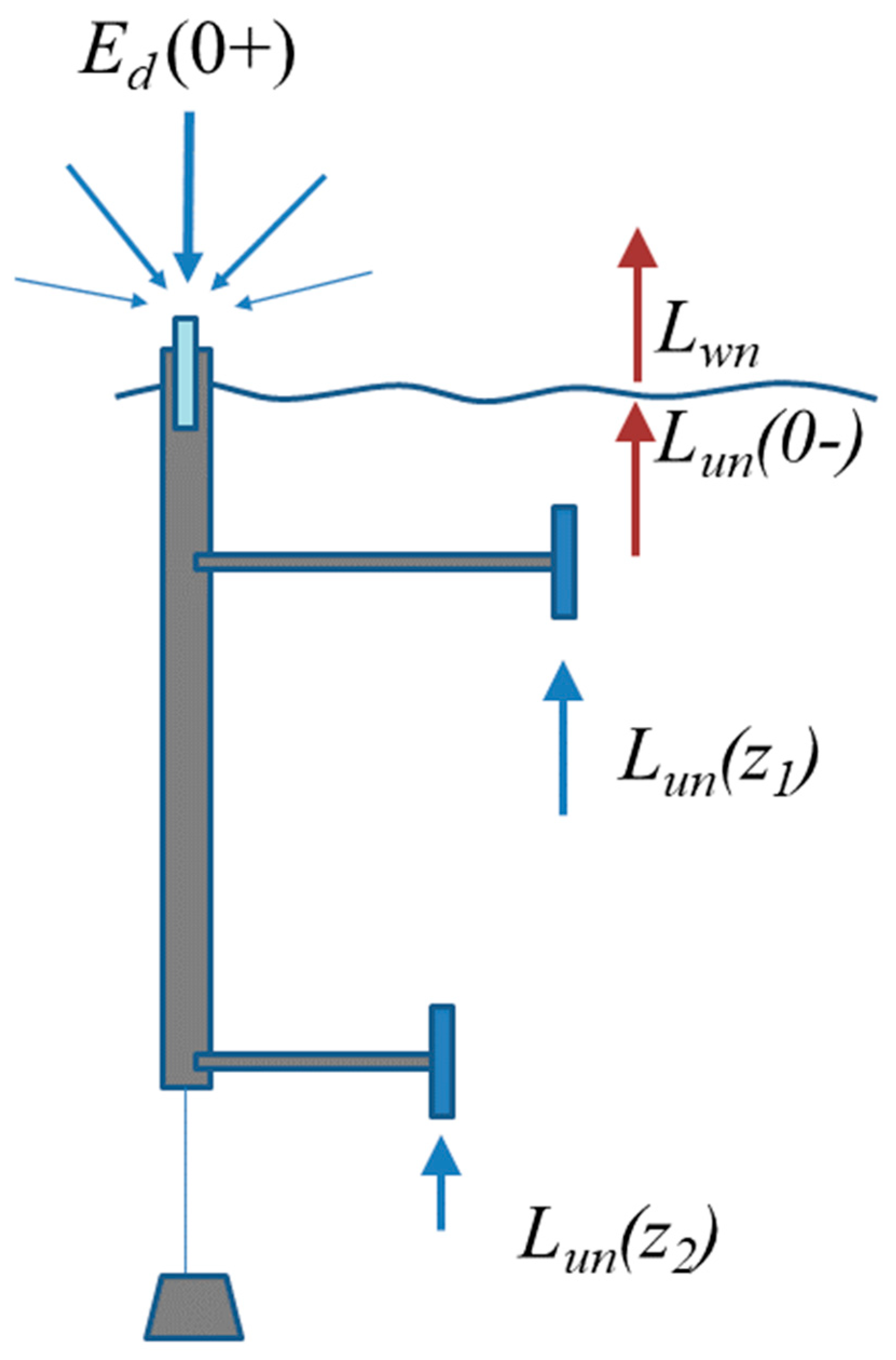
2. Underwater Radiometry—Fixed-Depth Measurements

2.1. Measurement Equation

In fixed-depth underwater radiometry, as typified by BOUSSOLE [25,26] and MOBY [27,28,29], radiometers are deployed underwater and attached to permanent floating structures, to measure nadir upwelling radiance, L u n ( z ) , at two or more depths, z = z 1 ,   z 2 ,   . —see Figure 3. A further measurement is made above water of downwelling irradiance, E d 0 + , to allow for calculation of R r s via Equation (1) and to monitor for possible variation of illumination conditions during the measurement. In the case of MOBY these L u n ( z ) measurements are made with z 1 = 1   m , z 2 = 5   m and z 3 = 9   m , while the BOUSSOLE system makes measurements at z 1 = 4   m , and z 2 = 9   m . Strictly speaking, these are fixed nominal depths because actual depth varies with tilt of structures and waves—see Section 2.2.5.
The nadir water-leaving radiance, L w n , is calculated by first estimating the nadir upwelling radiance just beneath the water surface, L u n ( 0 ) , by extrapolating from, preferably, the two shallowest depth measurements z 1 and z 2 assuming that the depth variation of L u n ( z ) between the surface, z = 0 , and z = z 2 , is exponential with constant diffuse attenuation coefficient for upwelling radiance, K L u . Thus, using the convention that depths beneath the water surface are considered as positive (but retaining the notation 0 for radiance just beneath the water surface),
L u n ( 0 ) = L u n ( z 1 , t 1 ) e x p [ K L u z 1 ]
with,
K L u = 1 z 2 z 1 l n [ L u n ( z 1 , t 1 ) L u n ( z 2 , t 2 ) E d 0 + ( t 2 ) E d 0 + ( t 1 ) ]
where E d 0 + ( t 1 ) and E d 0 + ( t 2 ) represent the downwelling irradiance measured at times t 1 and t 2 , corresponding to the times of measurement of L u n ( z 1 ) and L u n ( z 2 ) . If these radiances are measured at precisely the same time, as is the case for most such implementations, then Equation (4) simplifies to:
K L u = 1 z 2 z 1 l n [ L u n ( z 1 ) L u n ( z 2 ) ]
Finally, the water-leaving radiance is obtained from L u n ( 0 ) by propagating the latter across the water–air interface using,
L w n = T F n w 2 L u n ( 0 )
where T F is the Fresnel transmittance of radiance from water to air and n w is the refractive index of water. The refractive index of air, n a i r , is here assumed equal to unity. T F , which depends also on n w , can be easily calculated from Fresnel’s equations in the case of a flat water–air interface, e.g., [3] chapter 4.2, and has a typical value of 0.975 at normal incidence for oceanic water. T F / n w 2 takes a typical value of 0.543 for oceanic water [30]. In the case of a wave-roughened interface, by combining the reciprocity condition between radiance reflectance and transmittance coefficients [31] and the simulations of Figure 18 of [32], it was established that there is negligible (much less than 1%) difference for T F between a flat interface and a wave-roughened interface for wind speeds up to 20 m/s (neglecting the whitecaps and breaking waves that occur already at wind speeds much less than 20 m/s) [33]. However, for a more precise calculation of T F / n w 2 it is necessary to take account of wavelength, salinity and temperature variations of the refractive index, n w [34], both for oceanic waters [33] and for inland waters.
The choice of depth, z 1 , for the shallowest measurement is determined by the competing interests of a shallow depth to reduce errors due to propagation to the surface and reducing the chances of the shallow depth measurement broaching the surface. This choice is then dependent on the sea-state expected at the measurement location. The choice of depth, z 2 , for the second measurement is likewise a compromise between increasing z 2 z 1 , which reduces the uncertainty in the derived K L u , the possibility of an inhomogeneous water column over the measurement depth thus not being representative of K L u from z 1 to the surface, the natural variation in K L u due to inelastic processes [35], possible increased signal to noise because K L u is different at each wavelength, and an increase in overall length of the structure.
In addition to the time variation of illumination conditions due to time-varying sun zenith angle and diffuse atmospheric transmission (aerosols, clouds) which is accounted for in E d 0 + ( t 1 ) and E d 0 + ( t 2 ) , it is necessary to account for the temporal variation of underwater radiances L u n ( z 1 ) and L u n ( z 2 ) associated with waves at the air–water interface. Wave focusing and defocusing effects [36,37,38,39] and wave shadowing [40] may have very fast time scales, less than 1 s, and very short length scales, less than 1 cm, giving a time-varying 3D light field. These effects are reduced by averaging for L u n ( z 1 ) and L u n ( z 2 ) over a large number of measurements and making the extrapolation to depth 0 with the time-averaged values L u n ¯ ( z 1 ) and L u n ¯ ( z 2 ) or L u n ( z 1 ) ¯ / E d 0 + ( t 1 ) ¯ and L u n ( z 2 ) ¯ / E d 0 + ( t 2 ) ¯ (performing time-averaging on each parameter before taking the ratio). The probability density functions for E d 0 + ( t 1 ) and L u n ( z , t ) are skewed near the surface and approach normal distributions with depth [39,41]. For BOUSSOLE data, median averaging is used [26]. For MOBY mean averaging is used as defined in p21 of [28].
At high wind speed and wave height various problems may occur affecting measurement quality or usability. For example, whitecaps and/or breaking waves may affect the water-air Fresnel transmittance. Tilt may become high. Depth measurement may become uncertain or sensors may even emerge from water. Such conditions are usually excluded from satellite data products and validation analyses anyway because the air–water interface correction of satellite data is also not suited for high whitecap coverage and/or breaking wave conditions. There is no clear consensus on acceptable wind speed for the L w measurements, and this will clearly be dependent on the specific deployment equipment. A limit of 10 m/s would give an estimated whitecap coverage of 1% for fully-developed wind waves [42].

2.2. Protocol-Dependent Sources of Uncertainty

The protocol-related sources of uncertainty are described in the following subsections.

2.2.1. Non-Exponential Variation of Upwelling Radiance with Depth

The vertical variation of upwelling radiance between the lowest measurement depth and the air–water interface should be known
The essential assumption of exponential variation of L u n ( z ) used to extrapolate measurements from two fixed depths to just beneath the water surface is only an approximation of reality. Firstly, the water inherent optical properties themselves may vary with depth [43], for example because of vertical variability related to thermal stratification including a “Deep Chlorophyll Maximum”, or related to resuspended or river plume particles in coastal waters. Secondly, inelastic processes such as Raman scattering and fluorescence [35] cause non-exponential variation of radiance, particularly in the red and near infrared for Raman scattering. Thirdly, while for a homogeneous aquatic medium the attenuation with distance of a collimated beam of light can indeed be expected to be exponential the same does not hold for a diffuse light field. The angular distribution of upwelling light varies with depth, e.g., [44], and K L u depends on the angular distribution of light and so may be expected to vary with depth even for a homogeneous water column and without inelastic scattering—see Figures 9.5 and 9.6 of [3].
If a more appropriate non-exponential functional form can be found to represent the vertical variation of radiance with depth, e.g., by characterising vertical variability from profile measurements or from radiative transfer modelling [45], it is possible to modify Equation (3) to improve accuracy of the extrapolation, as suggested by using Case 1 models in Appendix A of [26] and [46].
The difficulties of non-exponential variation of upwelling radiance with depth become greater in waters or at wavelengths where the diffuse attenuation coefficient is high compared to the reciprocal of the measurement depths, e.g., in turbid waters and/or at red and near infrared wavelengths.
The uncertainty estimate associated with K L u can be validated by measuring K L u at high vertical resolution and close to the surface, e.g., from occasional shipborne campaigns.

2.2.2. Tilt Effects

The radiance sensors should be deployed vertically
Non-verticality of radiometers, e.g., caused by wave- or current-tilting of floating structures, will give uncertainty in the measurements of both E d 0 + and L u n ( z ) because of the anisotropic nature of the down- and up-welling light fields respectively. Therefore, it is necessary to measure the tilt of radiometers using fast response inclinometers and perform appropriate filtering of non-vertical data and/or averaging of data to reduce tilt effects.
The impact of tilt on E d 0 + measurements is discussed in [5].
Tilt can also affect the effective underwater radiance measurement depths, z i , which should therefore be measured continuously, e.g., using pressure sensors close to the optical sensors.
Obviously, minimisation of tilt can be a consideration in the design or in the location of validation measurement structures. As an example, the BOUSSOLE structure was designed to have low sensitivity to swell. The mean tilt of the buoy was measured as 4° (with 4° of pitching) for a 4.6 m swell of period 5.2 s [25] and data is rejected for tilt greater than 10° [26].

2.2.3. Self-Shading and/or Reflection from Radiometer and/or Superstructure

The light field should not be perturbed by the measurement radiometer and platform
In practice, the light field that is being measured is itself perturbed by the presence of solid objects such as the radiometers and the superstructure used to mount them. These perturbations are most pronounced when the water volume being measured (roughly defined horizontally by radiometer field of view and vertically by the diffuse attenuation coefficient, K L u ) is in some way shadowed from direct sun, although shadowing of downwelling skylight and side/back-reflection of down/upwelling light also contribute to optical perturbations.
Shading can lead to either under- or over-estimation of K L u depending on relative impacts at the depths z 1 and z 2 .
As regards the radiometers, self-shading can be minimised by using a sensor with fore-optics of small diameter compared to the mean free path of photons. This requirement becomes more challenging at longer wavelengths, such as in the near-infrared where the water absorption coefficient is high. A partial correction for self-shading effects for a radiometer with idealised geometry was proposed [47] for a concentric sensor, tested experimentally [48] and further generalized, including shallow water effects [49]. This correction requires measurement or estimation of IOPs.
As regards the superstructure, self-shading can be minimised by limiting the cross-section of the structure above the radiometers, e.g., by a sub-surface buoy [25] rather than surface buoy, and by increasing the distance between structure and radiometer, e.g., by the use of horizontal arms. The use of multiple redundant radiometers at the same depth but differently affected by superstructure and/or the measurement of superstructure azimuth and the identification/correction [50] of possible superstructure effects can also reduce superstructure shading uncertainty and/or be used to validate uncertainty estimates.

2.2.4. Bio-Fouling

The fore-optics of the radiance sensors should be kept clean
In addition to sensitivity changes inherent to the radiometer, modification of the transmissivity of the fore-optics can occur because of growth of algal films, particularly for long-term underwater deployments. Such bio-fouling can be mitigated: (a) by the use of shutters and/or wipers (provided the latter do not themselves scratch optical surfaces), (b) by use of copper surfaces and/or release of anti-fouling compounds close to the optical surface, e.g., p15 of [28], or by ultraviolet (UV-C) irradiation [51] (c) by limiting the duration of deployments between maintenance [26], (d) by monitoring optical surfaces in some way, e.g., occasional diver-operated underwater calibration lamps, e.g., p15 of [28], and (e) by regular diver cleaning of optics during the deployment.
In general, downward facing-sensors used to measure L u are much less prone to bio-fouling than upward-facing sensors used to measure E d [52].
An accumulation of bubbles on the horizontal surface of the L u fore-optics would also affect data and radiometers should be designed to avoid trapping of bubbles, e.g., by removal of any concave shields or collimators used for some above-water radiance sensors.
Fouling of the above-water upward-facing E d 0 + sensor is described in [5].
Residual uncertainty related to bio-fouling (taking account of any biofouling corrections, e.g., linear drift) can be estimated by comparing post-deployment calibrations before and after cleaning and by comparing pre-/post-cleaning operations by divers using a portable calibration source or by using L u time series in stable conditions [53].

2.2.5. Depth Measurement

The depth of radiance measurements should be accurately known
The measurement equation implies that the depth of measurement is accurately known. For large and permanent structures such as MOBY and BOUSSOLE, measurement of depth can be achieved quite precisely using pressure sensors (including a simultaneous above-water measurement of atmospheric pressure [54]) accounting for any time variation because of tilt and wave and current effects. If fixed-depth measurements are used at shorter vertical length scales, e.g., in shallow lakes or for measurement in high attenuation waters or wavelengths, depth measurements should be made sufficiently accurate so as to not contribute significantly to overall measurement uncertainty.

2.2.6. Fresnel Transmittance

The Fresnel transmittance for upwelling radiance should be accurately calculated
The Fresnel transmittance, T F , used to propagate upwelling nadir radiance across the water surface in Equation (6), is often assumed to have a constant value of 0.543 in sea water, but does vary with wavelength, salinity and temperature via the index of refraction of water—see also Section 2.1 and [33] where improvements on use of a constant value and uncertainties associated with T F are discussed.

2.2.7. Temporal Fluctuations

Temporal fluctuations associated with surface waves should be removed
Measurements are averaged over a certain interval of time (see Section 2.1) to remove as far as possible the fast variations associated with wave focusing/defocusing effects. Simulations can be performed [39,41] to assess the effectiveness of different averaging approaches/time intervals and any associated residual uncertainty.
If measurements from all sensors are not simultaneous the corresponding time corrections should be made and residual uncertainty estimated.

2.3. Variants on the Fixed-Depth Underwater Radiometric Method

Section 2 has been written primarily for MOBY/BOUSSOLE-style systems where radiometers are deployed at fixed underwater depths attached to a structure tethered to the sea bottom in an approximately constant geographical location (notwithstanding possible small horizontal movements associated with currents). Variants on this method, which are based on the same essential measurement equation, are briefly discussed here.
While the MOBY/BOUSSOLE superstructures are designed with small optical cross-section to minimise optical perturbations, buoys/platforms designed for other purposes, e.g., hydrographic measurements or navigation-related structures, may also be used for underwater radiometric measurements. The essential measurement equation and checklist of elements to be included in the uncertainty budget remain the same, although measurement uncertainties associated with superstructure shading will need to be very carefully assessed and will generally be much more significant.
Fixed-depth measurements may also be made from ships, e.g., when using radiometers with too slow a response time for fast vertical profiling. Again, the essential measurement equation and checklist of elements to be included in the uncertainty budget remain the same, although measurement uncertainties associated with ship shading/reflection will need to be very carefully assessed and will generally be much more significant unless the radiometers are somehow deployed at a sufficient distance from the ship.
At the time of writing, there are no known cases of multiple fixed-depth radiometric validation measurements being made from a horizontally moving platform. In general, horizontally moving platforms [24] (BioArgo, PROVAL, HARPOONS/Waveglider – see disclaimer at end before references) can also move vertically and so use a measurement technique based on high vertical resolution profiling, as described in Section 3.
The tethered attenuation chain colour sensors (TACCS) [55] is a variant on the fixed-depth measurement, where a single underwater L u n measurement, made at 0.5 m depth, is supplemented by a vertical chain of four downwelling irradiance sensors measuring E d ( z ) at multiple depths, in addition to the usual above-water E d 0 + measurement. The diffuse attenuation coefficient, K E d , that is derived from these E d ( z ) measurements is then used as an approximation of the K L u , that is needed to extrapolate L u n ( 0.5   m ) to L u n ( 0 ) . In one implementation [12] the E d ( z ) measurements are made at a lower spectral resolution that the L u n measurements, and K E d must, therefore, be interpolated/extrapolated spectrally. In other respects this variant on the fixed-depth underwater radiometry method has the same sources of uncertainty as listed in Section 2.2, except that further uncertainties must be assessed relating to the modelling of K L u from K E d , and the spectral interpolation/extrapolation of K E d .
In some implementations a single measurement of upwelling radiance is made close to the air–water interface [56]. The K L u required to extrapolate to the surface is then not measured but is either assumed zero or estimated using a model which takes the L u n spectrum as input (potentially repeated iteratively), giving a measurement uncertainty in both cases. In the optical floating system [57], measurements were made within 2 cm of the surface in very calm conditions. Vertical extrapolation of single depth near-surface measurements are discussed in Section 3E of [35].

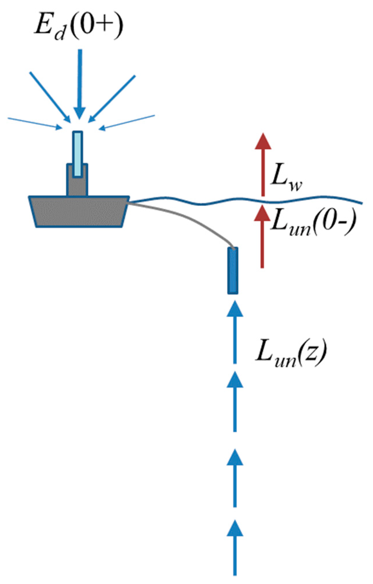
3. Underwater Radiometry—Vertical Profiles

Water-leaving radiance can also be measured using underwater radiometry based on vertical profiling—see Figure 4. This method has frequently been used in supervised deployments from ships [58] and can also be made from fixed platforms [43]. Theoretically, vertical profiling from a fixed platform could also be automated and unsupervised, although in practice long-term deployments of radiometers with moving underwater parts are vulnerable to mechanical failures. As an alternative, unsupervised vertical profiles can be carried out from horizontally drifting platforms or “floats” [59,60], as further described in Section 3.3.
The first vertical profile radiometric measurements were generally made from winches attached to ships [61]. However, it is clearly important to avoid as far as possible optical (shadow/reflection) [62] and hydrographic perturbations (ship wake, ship hull and propeller-induced mixing, bow wave, etc.) from the ship as well as vertical motion of optical sensors due to ship motion. It has been recommended to make measurements from the stern of a ship with the sun’s relative bearing aft of the beam at a minimum distance of 1.5 / K L u from the ship or at greater minimum distance when deploying off the beam of a large vessel—see Section 2.2, p8 of [63].
A popular method for getting radiometers away from ship perturbations is to float radiometers away a few tens of metres and then profile vertically using a specially-designed rocket-shaped free-fall platform [64]. More recently a new “kite” free-fall design allows slower profiling, closer to the water surface [54]. Remotely operated vehicles can also be used [65].
In view of such improvements in deployment hardware that have become commercially available over the last 15 years it is likely that fiducial reference measurements will generally not be made from shipborne winch deployments, although this is not formally precluded provided that the measurement is supported by a careful uncertainty analysis covering all perturbations specific to the ship/deployment method/water type combination, including, for example, measurements made at different distances from the ship and/or 3D optical model studies.
Vertical profiles can also be made from offshore structures, including fixed platforms, e.g., the WISPER system on the Aqua Alta Oceanographic Tower (AAOT) [43], or moored buoys with a vertical wire-mounted package. These structures have the advantage over shipborne winches of reduced tilt of radiometers and reduced hydrodynamic perturbations, although optical perturbations still need to be evaluated, e.g., by measurements made at different distances from the platform [66] and/or 3D optical model studies [67].

3.1. Measurement Equation

The fundamental measurement equation is similar to that used for fixed-depth measurements, except that measurements are now available for a range of depths z 1 z z 2 for estimation of the vertical variation of L u n ( z ) .
By definition of K L u , the diffuse attenuation coefficient for L u n :
L u n ( z , t 0 ) = L u n ( 0 , t 0 ) e 0 z K L u ( z ) d z
where z is positive underwater and increases with depth beneath the surface (but retaining the notation 0 for radiance just beneath the water surface) and t 0 is the time to which measurements are referred. This gives, after natural logarithm transformation and reorganisation:
ln [ L u n ( z , t 0 ) ] = l n [ L u n ( 0 , t 0 ) ] 0 z K L u ( z ) d z
If it is assumed that K L u is constant with depth over the depth range of measurements and up to the water surface, then this simplifies to:
ln [ L u n ( z , t 0 ) ] = l n [ L u n ( 0 , t 0 ) ] K L u z
L u n ( 0 , t 0 ) is then obtained from vertical profile measurements as the exponential of the intercept of a linear regression of ln [ L u n ( z , t 0 ) ] against z over a specified depth range.
Since measurements at different depths are made at slightly different times, t , the radiance measurements are first corrected for any variations in above-water downwelling irradiance by:
L u n ( z , t 0 ) = L u n ( z , t ) E d 0 + ( t 0 ) E d 0 + ( t )
Finally, the water-leaving radiance is obtained from L u n ( 0 , t 0 ) by propagating the latter across the water-air interface as in Equation (6).
A number of deployment and data-processing factors influence the quality of L u n ( 0 , t 0 ) derived from measurements of L u n ( z , t ) :
  • Measurements should be made as close as possible to the air–water interface to minimise the uncertainties associated with extrapolation from depth, particularly if there are vertical gradients of inherent optical properties or for wavelengths/waters with high vertical attenuation. Very near-surface measurements are complicated by waves, which affect radiometer tilt and vertical positioning as well as the radiance field itself (focusing/defocusing). To deal with this, new profiling platforms have been designed for very slow and stable sampling close to the surface [54].
  • Sufficient measurements are needed for each depth (interval) to ensure that wave focusing and defocusing effects can be removed, implying that profiling speed should be sufficiently slow, adding to the time required to make a cast, a practical consideration, and the possibility of temporal variation of illumination conditions, a data quality consideration.
  • The vertical profiling speed should be matched to the acquisition rate of the radiometers to ensure that the depth z of each measurement can be determined with sufficient accuracy.
  • The depth range z 1 z z 2 chosen for data processing is “the key element in extracting accurate subsurface data from in-water profiles” [68]. z 1 should be chosen sufficiently large to avoid problems of near-surface tilt, wave focusing/defocusing and bubbles, but sufficiently small to limit uncertainties associated with extrapolation to the surface, particularly for high attenuation waters/wavelengths. Any depth interval with significant ship/superstructure shadowing must also be avoided. In practice, the choice of depth range is generally made subjectively [11] because of the difficulty to automate such thinking.
  • The depth range z 1 z z 2 used in data processing can be wavelength-dependent (unlike for the fixed-depth method of Section 2), e.g., using optical depth to set z 2 differently at each wavelength.
  • Different mathematical methods used to perform the regression analysis for Equation (9) and different methods for filtering outliers [69] may give quite different results. Such considerations were analysed in detail in the Round Robin experiments documented by [11].
  • For measurements with significant temporal variability of E d 0 + ( t ) , some time filtering of E d 0 + ( t ) may be needed before application of Equation (10). For example, E d 0 + ( t 0 ) may be chosen as the median of E d 0 + ( t ) over the measurement interval or, for ship-induced periodic variability, E d 0 + ( t ) may be first linearly fitted as function of t .
For profiling systems where the upcast is made by applying tension to a wire, only downcast (“free-fall”) data is used to avoid irregular motion and high tilt.

3.2. Protocol-Dependent Sources of Uncertainty

The protocol-related sources of uncertainty are described here for the case of a profiling system that is supposed to be fixed, or almost fixed, in horizontal space, e.g., tethered to a ship or an offshore platform. Additional considerations to account for significant horizontal movements, e.g., from glider platforms, are summarised in Section 3.3.

3.2.1. Non-Exponential Variation of Upwelling Radiance with Depth

The vertical variation of upwelling radiance between the highest measurement depth and the air–water interface should be known
The essential assumption of exponential variation of L u n ( z ) from the measurement depth range z 1 z z 2 to just beneath the air–water interface is clearly an approximation of reality. This assumption will cause uncertainties in conditions of near-surface optical stratification, inelastic scattering (Raman, fluorescence) and variability of the angular distribution of upwelling radiance, as already described in Section 2.2.1 for fixed-depth radiometry.
The uncertainty associated with non-exponential variation of L u n ( z ) can be assessed for the measurement range z 1 z z 2 by considering the goodness-of-fit of Equation (8), after suitable filtering of temporal variability and taking account of realistic uncertainties. For 0 z z 1 , between the measurement range and the surface, potential non-exponential variation of L u n ( z ) can be assessed by model studies [45]. If this non-exponential variation is already considered in the fitting methodology, then the uncertainty is reduced to the residual uncertainty associated with the difference between the true non-exponential variation of L u n ( z ) and the estimated non-exponential variation.
Clearly z 1 should be kept as shallow as possible, within constraints of deployment, tilt contamination and temporal variability, particularly if there may be near-surface stratification of the water column.

3.2.2. Tilt Effects

The radiance sensor should be deployed vertically
Non-verticality of radiometers, e.g., caused by wave-tilting of free-fall platforms or ship winch-deployed frames, gives uncertainty in the measurements of L u n ( z , t ) because of the anisotropic nature of upwelling light fields. It is, therefore, necessary to measure the tilt of radiometers using fast response inclinometers and perform appropriate filtering of non-vertical data and/or averaging of data to reduce tilt effects [69].
The uncertainty associated with tilt effects can be estimated by reprocessing of oversampled vertical profile measurements with different thresholds for removal of non-vertical data and by 3D optical model simulations.
The impact of tilt on E d 0 + measurements is discussed in [5].
Obviously, minimisation of tilt should be a consideration in the design of deployment hardware. Vertical profiles carried out from fixed platforms suffer less from such tilt effects. The “rocket-shaped” free fall platforms may suffer from high tilt, particularly in near-surface waters and high wave conditions. The new designs of ”kite-shaped“ profilers [70] and autonomous profiling floats [60] have significantly reduced tilt.

3.2.3. Self-Shading from Radiometers and/or Superstructure

The light field should not be perturbed by the measurement radiometers and platform
In practice, the light field that is being measured is itself perturbed by the presence of solid objects such as the radiometers and the superstructure used to mount them, as discussed previously in Section 2.2.3 for fixed-depth underwater radiometry. For free-fall radiometer platforms, the considerations and corrections discussed in Section 2.2.3 as regards self-shading from the radiometer collector and from the mounting frame are relevant also for vertical profiling. For ship-tethered free-falling radiometers with an off-centre L u sensor, azimuthal rotation should be controlled to have the L u sensor on the sunny side.
Redundant deployment of two sensors at the same depth but on different sides of a profiling platform can help identify and remove the data worst affected by platform shading. Knowledge of platform azimuth with respect to sun can help assess such effects [60].
For ship- or fixed platform-deployed vertical profiling radiometers, superstructure shading/reflection effects may be considerable and should be carefully limited, by maximising horizontal distance from the structure. Uncertainties should be estimated, e.g., by radiative transfer modelling [67,71] and/or by in situ measurements at different distances from the structure.

3.2.4. Bio-Fouling

The fore-optics of the radiance sensor should be kept clean
Supervised underwater radiometric measurements generally do not suffer from bio-fouling provided that fore-optics are kept clean between deployments.
Fouling of the above-water upward-facing E d 0 + sensor is described in [5].
Unsupervised fixed location vertical profiling measurements are rare but would suffer from similar problems to those described in Section 2.2.4 for fixed-depth measurements.
Horizontally drifting vertical profiling systems (Section 3.3) may arrange to spend most time at great depth to minimise bio-fouling [24]. Residual bio-fouling uncertainties (after any biofouling correction, e.g. linear drift) can be estimated by comparing pre- and post-deployment calibrations, although recovery of horizontally drifting systems is not always possible.

3.2.5. Depth Measurement

The depth of radiance measurements should be accurately known
The measurement equation implies that the depth of measurement is precisely known by a fast response and appropriately calibrated pressure sensor located close to the optical sensor. Any permanent vertical shift between depth sensor and optical sensor must be corrected and any tilt-induced vertical difference between depth and optical measurements must be included in the uncertainty estimate. Accurate measurement of depth and associated uncertainties is needed, including referencing to surface atmospheric pressure at the moment of profiling (pressure “taring”) and temperature-sensitivity of pressure transducers—see Section 5.2 of [54].

3.2.6. Fresnel Transmittance

The Fresnel transmittance for upwelling radiance should be accurately calculated

3.2.7. Temporal Fluctuations

Temporal fluctuations associated with surface waves should be removed
The removal of temporal fluctuations in L u n ( z , t ) , e.g., from wave focusing/defocusing is complicated for vertical profile measurements because both the light field and the measurement depth, z , vary with t , and because measurements may be affected by both natural variability (wave effects, water variability) and by deployment-related variability (e.g., tilt and vertical wave motions).
If all other factors (above-water illumination, water optical properties) are assumed invariant in time during the measurements, or suitably corrected, and L u n ( z , t ) is assumed to be tilt-free after filtering, then natural variability caused by wave effects [72] can be minimised by performing sufficient measurements to allow adequate averaging. This can be achieved by slow profiling [54,73] or, if this is not possible, by multicasting [68].
The uncertainty associated with all sources of temporal fluctuations must be estimated, e.g., by testing alternative data processing options on oversampled measurements and by 4D optical simulations [45]. Uncertainty estimates should be validated, e.g., by measurement intercomparison exercises [12].

3.3. Variants on the Vertical Profiling Underwater Radiometric Method

Following on from the success of the Argo float network designed for physical oceanography, a number of horizontally-drifting vertical-profiling radiometer platforms have been designed for long-term unsupervised measurement of optical properties [24,59,60]. Such floats, when suitably networked, allow for much better spatial coverage of the oceans (but not shallow seas or inland waters). Typically, the radiometer will park at great depth during most of the day and night (to reduce bio-fouling) and perform one or more vertical profiles per day (rising at about 4 cm/s to 10 cm/s or slower), potentially timed to match the acquisition times of specific ocean colour sensors. Such systems can also combine vertical profiling with near-surface fixed-depth ”drifting buoy“ measurements, thus falling within both Section 2 and Section 3 of this document and allowing the vertical profile K L u measurements to be used for the near-surface single fixed-depth measurements.
The essential measurement equation and sources of uncertainty for such measurements are the same as for other vertically profiling radiometers. As for all unsupervised measurements, biofouling, particularly for the upward-facing E d 0 + measurement [5], may be a significant source of uncertainty, especially if the radiometer cannot be recovered for post-deployment calibration. On the other hand, the possibility of diving deep limits exposure to biofouling.
In contrast to vertical profile measurements made from ships or fixed offshore structures, drifting floats generally do not have a permanent above-water radiometer for E d 0 + ( t ) and so there will be an additional uncertainty associated with possible time variation of illumination conditions during the vertical profile, although the latter may also be reduced by analysis of the E d ( z , t ) profile data [74].
Floats can also accommodate radiometers on horizontal arms and redundant radiometers to provide additional constraints on sensor drift and shading by platform [60].

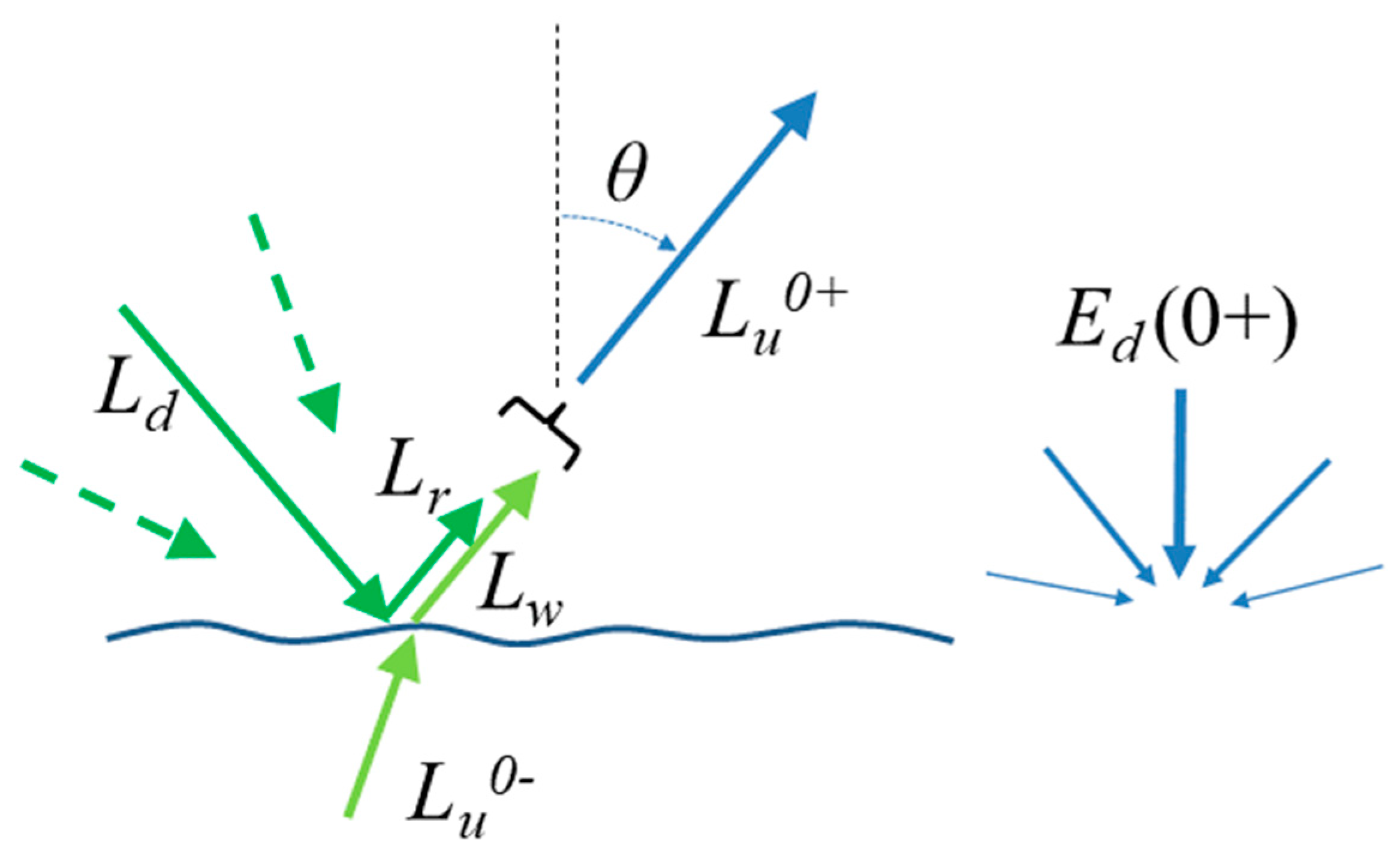
4. Above-Water Radiometry with Sky Radiance Measurement and Skyglint Removal

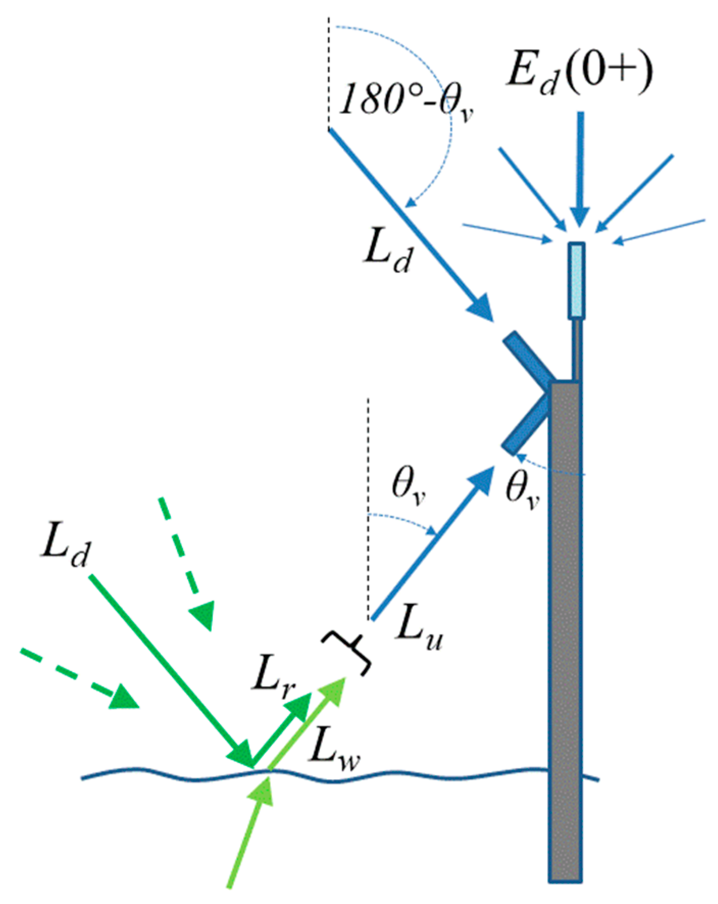
4.1. Measurement Equation

In above-water radiometry one or two radiometers are deployed above water from a ship or fixed structure to measure (a) upwelling radiance, L u ( 0 + ,   θ v , Δ φ ) , at a suitable viewing nadir angle, θ v < 90 ° , and viewing azimuth angle relative to sun, Δ φ , and (b) downward (sky) radiance, L d ( 0 + ,   180 ° θ v , Δ φ ) , in the “mirror” direction which reflects at the air–water interface into the water-viewing direction—see Figure 5.
Then the water-leaving radiance in the water-viewing direction is estimated from the measurement equation:
L w ( θ v , Δ φ ) = L u ( 0 + ,   θ v , Δ φ ) L r ( θ v , Δ φ )
where the skyglint radiance, L r , which cannot be measured directly, is typically estimated as a multiple of the downwelling sky radiance, L d , by
L r ( θ v , Δ φ ) = ρ F L d ( 0 + ,   180 ° θ v , Δ φ )
where ρ F is a coefficient that represents the fraction of incident skylight that is reflected back towards the water-viewing sensor at the air–water interface and is the Fresnel reflectance coefficient for a flat water surface, or is called here the “effective Fresnel reflectance coefficient” for a roughened water surface.
The second part of this measurement Equation (12), which forms the basis of this protocol, is adopted as a pragmatic way of estimating and removing the upwelling radiance that originates from reflection at the air–water interface. However, it is well understood that such radiance may originate from portions of the sky dome other than the portion that is actually measured, as defined by ( 180 ° θ v , Δ φ ) and the field of view of the L d radiometer. L r may include reflection of direct sun glint—see Figures 1 and 2 of [75] and Equation (1) of [76]. This is discussed further in Section 4.2.1. In reality, the right hand side of (12) is an approximation of the convolution of sky radiances for the full hemisphere with the wave slope statistics, defining the probability of encountering a part of the air–water interface that reflects specularly into the direction ( θ v , Δ φ ) , and the Fresnel reflectance coefficient for the corresponding incidence angle—see Chapter 4 and Equation (4.3) of [3] or Equation (3) of [77] for a complete description.
In the case of a flat water surface with only specular reflection processes (i.e., no whitecaps or other diffuse reflection processes) and with unpolarised downwelling light, and for an infinitesimally small sensor field of view, ρ F is simply given by the Fresnel reflectance equation and is plotted in Figure 6:
ρ F ( θ v ) = 1 2 { [ s i n ( θ v θ t ) s i n ( θ v + θ t ) ] 2 + [ t a n ( θ v θ t ) t a n ( θ v + θ t ) ] 2 }
where θ v is the viewing nadir angle (“above-water incidence angle”) and θ t is the angle of light transmitted to below water after refraction:
θ t = 180 ° s i n 1 ( s i n θ v / n w )
where n w is the index of refraction of water with respect to air and is often approximated by the value 1.34 but does also vary with salinity, temperature and wavelength [3].
For nadir-viewing, θ v = 0 , and Equation (13) is replaced by:
ρ F ( 0 ) = ( n w 1 n w + 1 ) 2
The nadir viewing angle variation of ρ F is illustrated for this flat-water surface and for modelled wavy water surfaces in Figure 6.
In reality:
  • The water surface is not flat but is a wavy surface [32] implying that (a) the portion of sky reflected into the water-viewing direction may come from directions other than L d ( 0 + ,   180 ° θ v , Δ φ ) [75], and that (b) the incidence angle required for calculation of the Fresnel coefficient is different from θ v , with spatial variation of the incidence angle within the sensor field of view that increases with wave inclination.
  • The downwelling light is not unpolarised, but, particularly for the molecularly scattered “Rayleigh” component at 90° scattering angle from the sun, may be strongly polarised [78].
  • Some radiometers have a field of view that can be quite significant, e.g., >10°, meaning that the measurements L u 0 + ( 0 + ,   θ v , Δ φ ) and L d ( 0 + , 180 ° θ v , Δ φ ) are weighted averages over a range of viewing angles ( θ v , Δ φ ) and the model for ρ F may need to account for different incidence angles even for a flat water surface.
These considerations are dealt with in detail in the following Sections and their references.
As regards the classification of methods for measuring L w , it is suggested here to drop the Method1/2/3 above-water radiometry classification used in the NASA Ocean Optics 2003 protocols [79] mainly for the E d 0 + measurement and in future classify the above-water L w measurements according to viewing geometry, measuring radiance with:
  • Viewing nadir angle, e.g., θ v = 0 ° (pointing towards nadir) or θ v = 40 ° or “other”.
  • Viewing relative azimuth angle to sun for off-nadir measurements, e.g., Δ φ = 90 ° or Δ φ = 135 ° or “other”.
and
  • The method used to estimate skylight reflected at the air–water interface.
In general nadir-viewing is avoided because of the high uncertainties associated with skyglint removal in geometries close to sunglint [75] and because of difficulties in avoiding optical perturbation from the ship/platform. However, there may be situations where nadir-viewing can be acceptable (e.g., mirror-flat lakes, sensors deployed well above water surface from an optically small structure, high sun zenith angle) provided that uncertainties are careful assessed and validated.
The measurement of polarized upwelling radiance [80,81] is considered as a variant of the above-water L w method – see Section 4.3.
In view of the quite different measurement uncertainties, the skylight-blocked approach (SBA) [76,82] is treated in the separate Section 5.

Temporal Processing of Radiance Measurements

Measurement of both sky radiance and water radiance involves time integration for each individual measurement and replicate measurements which are subsequently processed to yield a single value for L u ¯ ( 0 + ,   θ v , Δ φ ) and L d ¯ ( 0 + , 180 °   θ v , Δ φ ) where the overbar represents the multitemporal measurement, typically called “time-average”, although the temporal processing may be different from a mean average and will generally involve prior outlier removal or time series based quality control.
The integration time depends on the radiometer concept and the brightness of the target. Filter-wheel radiometers generally measure fast, typically at many hertz, whereas spectrometer-based systems may be fast, e.g., 8 ms to 32 ms, for bright targets such as the sky, but much slower, e.g., integration time of 1 s to 4 s, for darker targets such as water.
For the sky radiance measurement, L d ¯ ( 0 + ,   180 ° θ v , Δ φ ) , a small number of replicate measurements should be sufficient. If the sky conditions are good (clear blue sky) then 3 to 5 replicates should be sufficient to establish this and provide a mean average and standard deviation for this parameter. If the sky conditions are not good (e.g., scattered clouds and/or partially obscured sun) then this will also be immediately apparent from even a low, e.g., 3 to 5, number of replicates either in the standard deviation or in the magnitude of L d ¯ / E d 0 + at 750 nm, which will be much higher than that of an ideal sky model, see Web Appendix 1 of [22].
For the water radiance measurement, L u ¯ ( 0 + ,   θ v , Δ φ ) , a much larger number of replicate measurements is needed because of the rapid and large temporal variations associated with surface gravity waves. These variations include the darkening/brightening effect of large surface gravity waves oriented towards/away from the sensor (because of air–water interface reflectance differences and/or reflection of brighter/darker portions of the sky) as well as the very bright, small and fast sunglint “flashes” from specular reflectance of direct sun at suitably oriented capillary wave facets, particularly when viewing at low θ v θ 0 , low Δ φ and for high wave amplitudes. The temporal processing of L u ( 0 + ,   θ v , Δ φ ) measurements should also depend on the integration time of each measurement and may be linked to the method for estimation of ρ F . For example, a temporal processing method has been used for a rapidly sampling, small field of view radiometer that retains the minimal values of L u ( 0 + ,   θ v , Δ φ ) over a number of replicates and uses a flat sea model for ρ F using the principle that sunglint flashes and brighter waves can be resolved and eliminated by the minimum filter [83]. A different approach was suggested [75] for the case effectively of a slowly sampling radiometer where the contributions of different wave facets cannot be isolated but are effectively averaged in time (and possibly space, depending on the field of view and distance from the water surface) for each individual L u ( 0 + ,   θ v , Δ φ ) measurement. In the latter case a quite different value of ρ F may be required from that of the flat water surface model of Equation (13)—see Figure 2 of [84].

4.2. Protocol-Dependent Sources of Uncertainty

The protocol-related sources of uncertainty are described in the following subsections.

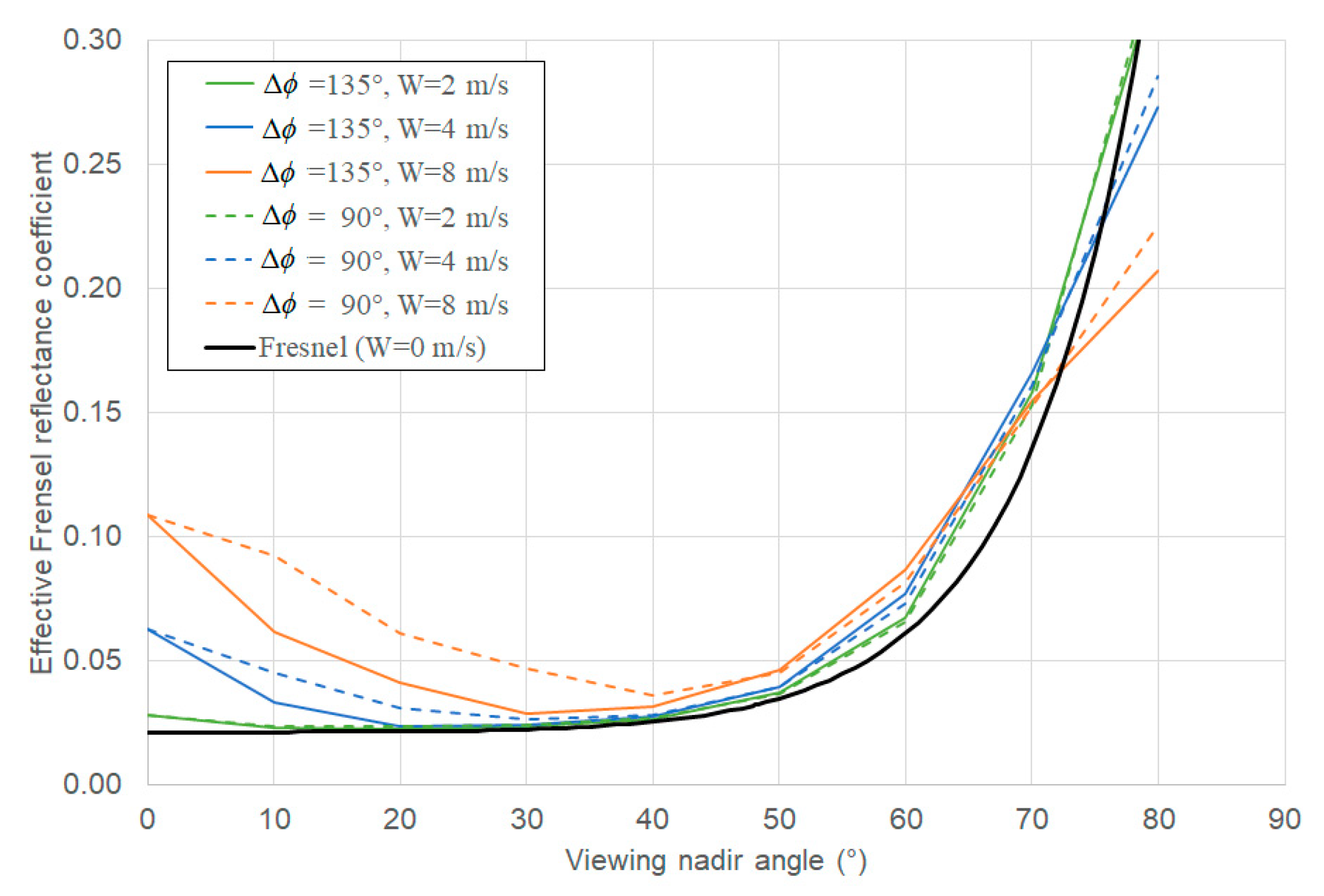
4.2.1. Estimation of Reflected Skylight

Upwelling radiance from reflection at the air–water interface (skyglint/sunglint) should be removed
The most critical aspect of above-water measurements of L w lies in the removal of skylight reflected at the air–water interface, represented by the coefficient ρ F in Equation (11). For waters or wavelengths where R r s is low, the right-hand side of (11) can be the difference of two values which are much larger than the left hand side. For example, in clear waters in the near infrared, L w may be negligibly small whereas L u ( 0 + ,   θ v , Δ φ ) and ρ F L d ( 0 + ,   180 ° θ v , Δ φ ) are not. Any uncertainty in ρ F is then greatly amplified when taking the difference. It is important to note that the uncertainty on ρ F L d ( 0 + ,   180 ° θ v , Δ φ ) is an absolute uncertainty for L w [22] that is unrelated to the value of L w itself and so becomes more important in relative terms as L w decreases. This is in contrast to most radiometer-related uncertainties (calibration, E d 0 + cosine response, radiometer thermal sensitivity, etc.) which are relative uncertainties that can be expressed as a percentage of the desired parameter, L w or R r s .
In view of the importance of estimating L r or the product ρ F L d ( 0 + ,   180 ° θ v , Δ φ ) there is quite large diversity of approaches. In the crudest approach, ρ F is simply taken from the flat sea Equation (13) and therefore generates large uncertainties that may be strongly positively biased for L w . For waters with low red or near infrared reflectance, a further “residual” correction may be applied [85], assuming that L w = 0 for a suitable wavelength, λ 0 , and that L r ( θ v , Δ φ ) has spectral variation given by L d ( 0 + ,   180 ° θ v , Δ φ ) .
Such an approach may also be used in highly absorbing waters at both ultraviolet and near infrared wavelengths to provide two fixed points at each extreme of the spectrum for a full spectrum construction of L r ( θ v , Δ φ ) [86].
For brighter waters, a wavelength λ 0 with negligible L w may not exist and, in an approach analogous to turbid water aerosol correction algorithms, a “turbid water” residual correction was proposed [87] based on measurements at 715 nm and 735 nm. This approach was generalised for any pair of near infrared wavelength [88], but was suggested for use in quality control/uncertainty estimation rather than data correction.
Scalar radiative transfer simulations were carried out [75] to establish ρ F as function of sun and viewing geometry ( θ 0 , θ v , Δ φ v ) and wind speed at a height of 10 m above the water, W , assuming a Cox-Munk relationship [89] between surface wave field and wind speed. In general, the directionality of the wave field (in particular the azimuth angle between wind direction and sun) is not accounted for when applying such corrections, although variability with wind direction has been observed [89] and this directionality may affect data [40]. In the case of fetch-limited inland waters W will typically be set to zero or a small value, since the Cox–Munk relationship will not apply. Similarly in overcast conditions (not very relevant for satellite validation) the dependence on surface wave field and/or W is also less strong and a constant value of ρ F = 0.028 has been proposed [75]. The table of values calculated for ρ F as function of ( θ 0 , θ v , Δ φ v ) and W is provided for download at [90], together with an updated table including polarisation effects [91], as described below.
It has been noted [76] that, since contributions to L r (   θ v , Δ φ ) arise from different portions of the sky (including direct sun) when the surface is not perfectly flat, these will have different spectral shapes from the L d ( 0 + ,   180 ° θ v , Δ φ ) that is measured. This effect is not accounted for in the simulations of [75] where the model assumes the same colour of the sky in all directions.
Sky radiance measured over small inland waters may include a component of light which has been scattered by land and then further backscattered in the atmosphere, giving, near vegetated land, a stronger near infrared contribution than typical oceanic skies [92].
For measurements made in inland waters very close to trees or in the vicinity of steep mountains, the sky radiance measurement may even include directly light from objects that are not sky—such problems could be mitigated by choosing the most favourable of the two possible relative azimuth angles (left or right of sun) although it will clearly be very challenging to make good measurements in such circumstances of highly anisotropic downwelling “skydome” hemisphere.
It has been shown that ρ F is, in reality, significantly lower than that in the simulations of [75] because the downward radiance is not unpolarized [93]. This effect is particularly strong when viewing near the Brewster angle of about 53°. Further simulations do take account of such polarisation effects [91,94] and the impact of aerosols, showing the further dependency of ρ F on aerosol optical thickness [95]. Other simulations take account of polarisation effects and also demonstrate that quite different mean surface slopes and hence quite different surface reflectance factors can arise from a single wind speed [40].
In one study, also taking account of polarization, the sunglint and skyglint components of light reflected at the air–water interface are treated separately [77]. In that formulation, the reflected light is still modelled as a multiple of the measured incident skylight in the sky-viewing direction, L d ( 0 + ,   180 ° θ v , Δ φ ) , but the air–water interface reflection coefficient, ρ F , is split into two reflection coefficients, ρ s u n ( λ ) , and ρ s k y ( λ ) representing respectively the sunglint and skyglint contributions. Although these coefficients are considered as “spectrally varying” in that paper it is noted that this “spectral variation” is a model to correct for the fact that the L d ( 0 + ,   180 ° θ v , Δ φ ) measurement is not representative of the spectral variation of sky radiances from all portions of sky (including direct sun) that are reflected towards the water-viewing sensor. The true spectral variation of the flat sea Fresnel coefficient, because of salinity and temperature related variation of the refractive index of water, is less significant (but also accounted for in that study). Using this decomposition of L r ( θ v , Δ φ ) into skyglint and direct sunglint components [77], the spectral variation of the latter follows the spectral radiance of the direct sun radiance, which is clearly different from the measured sky radiance L d ( 0 + ,   180 ° θ v , Δ φ ) and may be closer in spectral variation to that of the measured downwelling irradiance, E d 0 + .
The effective air–water interface reflection coefficient, ρ F , has been modelled for a continuum of viewing nadir and azimuth angles, sun zenith angles and wind speeds [84]. The impact of aerosol optical thickness on ρ F was demonstrated and it was recommended that above-water radiometric measurements be accompanied by measurements of aerosol optical thickness.
In a way that is analogous with the development of full spectrum coupled ocean-atmosphere modelling in satellite data atmospheric correction algorithms, more complex schemes have been proposed for taking account of the expected spectral shapes of L w and ρ F L d ( 0 + , 180 ° θ v , Δ φ ) . e.g., [96].
For hyperspectral measurements it has been proposed [97] to use the fact that R r s can be expected to be spectrally quite smooth whereas both L u ( 0 + ,   θ v , Δ φ ) and ρ F L d ( 0 + ,   180 ° θ v , Δ φ ) are affected by atmospheric absorption features. Thus ρ F can be constrained or estimated as the value that will yield a spectrally smooth R r s .
While there have been many recent and diverse developments for the removal of skyglint in data post-processing, the acquisition geometry of θ v = 40 ° viewing angle for the water and 180 ° θ v = 140 ° viewing angle for the sky observations, as proposed in [75] and endorsed by [79], remains a very robust and practical approach: viewing angles below 40° are more often associated with the impact of sunglint effects [84], while at viewing angles larger than 40° the reflectance coefficient becomes more sensitive to the small changes of the viewing angle as clearly follows from Figure 6. In addition, for moderate wind speeds the impact of aerosol optical thickness and polarization on the reflectance coefficient is typically smaller than for other viewing angles [84]. The azimuth angle for the water and sky observations should be closely monitored and should be the same for both measurements because of the significant azimuthal gradient of the sky radiance [84].
Using a hyperspectral imaging camera, relative uncertainties for L w have been estimated arising from L r correction for the spectral range 450 nm to 900 nm and for viewing angles 20° to 60° as a function of wind speed [84]. These uncertainties are most critical at blue wavelengths for waters with low blue reflectance, typical of coastal waters, where L r / L w is greatest. That study [84] also showed that both water and sky radiance measurements are not sensitive to the field of view (FOV) of the optics for FOV between 4° and 31.2° for measurements made at between 6 m and 8 m above water level with integration time 20 ms to 50 ms for a wind speed of 5.6 m/s.
If L u and L d are measured with different radiometers, e.g., as in the implementation of [22], then the differences between the radiometer sensitivities as a function of wavelength will add some measurement uncertainty for the spectrally-binned L w —this is often visible in hyperspectral measurements where narrow and strong atmospheric absorption features, such as oxygen absorption near 762 nm, lead to “blips” in L w or R r s spectra.
In view of the wide diversity of approaches for estimation of ρ F [98] and continued research into methodological improvements, the present document does not intend to prescribe a single protocol for estimating L r (   θ v , Δ φ ) or ρ F in FRM measurements. In fact, for most data acquisition protocols, different methods for estimating ρ F or L r (   θ v , Δ φ ) can be applied in post-processing and could be applied to historical data. Rather the approach of the current document is merely to insist that the uncertainties of any approach be thoroughly estimated and validated.
One method for estimation of uncertainties associated with L r ( θ v , Δ φ ) removal is to consider the spectral consistency of R r s ( θ v , Δ φ ) in the near infrared. For clear waters and at sufficiently long wavelength R r s can be assumed zero and any offset in measurements can be used as an estimator of total measurement uncertainty, provided this information has not already been used to perform a “residual correction” of data—this approach was suggested by [99], although in their study the uncertainty was expected to come more from ship perturbations (Section 4.2.3) than from L r ( θ v , Δ φ ) removal. The approach was extended [88] for moderately turbid waters, where R r s is non-zero in the near infrared, but adopts a spectral shape determined primarily by the pure water absorption coefficient [22].

4.2.2. Tilt and Heading Effects

Radiance measurements should be made at exactly the prescribed viewing nadir and relative azimuth angles
The uncertainty in the pointing angle of radiometers used for measuring both L u ( 0 + ,   θ v , Δ φ ) and L d ( 0 + ,   180 ° θ v , Δ φ ) must be propagated through to give an uncertainty for L w ( θ v , Δ φ ) .
When operating from boats inaccuracies in pointing angle may arise from (a) the initial setup and levelling of radiometers for the “at rest” balancing of the boat, and any resetting that is required during a campaign, e.g., because of changes in boat balance (ballasting, fuel and water tanks, deployment of equipment overboard by crane, etc.) and; (b) pitch and roll, which may easily reach 10° or more in heavy sea states or for small boats. Above-water radiometry from most fixed platforms is not significantly affected by wave- or wind-induced tilt and angular accuracy of <1° is easily achieved with a rigid structure, but can be exceeded for a flexible mast.
The impact of tilt can be estimated and reduced by: (a) measuring the inclination of the radiometers or the mounting platform/ship with a fast response well-calibrated inclinometer and removing all data where tilt exceeds a user-defined threshold; and (b) calculating the mean average and standard deviation of a time series of replicate measurements.
For the L u ( 0 + ,   θ v , Δ φ ) measurement, tilt, particularly any setup angle error, will affect the effective angle of data for L w ( θ v , Δ φ ) and hence any bidirectional corrections that may subsequently be applied to reproject data to nadir-viewing or to the satellite-viewing geometry. However, the related uncertainties will generally be low provided that data are sufficiently tilt-thresholded before processing. Tilt will also affect the effective incidence angle for calculation of the effective Fresnel reflectance, particularly for high wave conditions and when viewing at high viewing nadir angle such as >40°.
While pointing away from the sun azimuth minimizes the azimuthal variation of effective Fresnel reflectance, the deviation between nominal ∆φ and actual ∆φ provides an additional source of uncertainty. The actual ∆φ should therefore be measured, typically using a magnetic compass and modelled sun azimuth angle for shipborne measurements. For unsupervised deployments a reference azimuth is generally set during installation by sun-pointing and is regularly checked.
For the L d ( 0 + ,   180 ° θ v , Δ φ ) measurement, tilt will result in a different portion of the sky being measured from the sky that is effectively reflected by the air–water interface into the water-viewing sensor.

4.2.3. Self-Shading from Radiometers and/or Superstructure

The light field should not be perturbed by the measurement platform
Measurements from boat- and platform-mounted water-viewing radiometers may be contaminated by optical perturbations from the boat/platform. These perturbations are most pronounced when the water volume being measured is in some way shadowed from direct sun, although shadowing of downwelling skylight and reflection of downwelling light from structures also contribute to optical perturbations.
For the above-water optical perturbations to E d , one can imagine operating a fish-eye camera pointing vertically upwards from the water surface at the centre of the radiometer field of view—see Figures 2 and 3 of [5] except that, in the context of impact on the L w measurement, the location for such photos is the water surface target. Anything in the hemispherical picture that is not the sun/sky represents an optical perturbation, that will be wavelength-dependent and may be either positive or negative, e.g., blue sky replaced by part of the ship. This effect is most important for objects close to zenith because of their greater contribution to the cosine-weighted integral of E d (see Equation 2 of [5]), for objects close to the sun where sky radiance is greatest and for objects which occupy a large solid angle of the sky.
The ship/platform may also throw a shadow (or reflections) that affect the underwater light field and hence L w ( θ v , Δ φ ) , particularly in clear waters and/or for wavelengths with low diffuse attenuation coefficient.
Optical perturbations from the ship/platform are generally reduced in the system design by:
  • Mounting the water-viewing radiometer as high as possible, e.g., on a telescopic mast [100,101];
  • Choosing the radiometer mounting position to limit optical perturbations, e.g., at the prow of a ship, facing forward [22,102] or at a corner of a fixed offshore platform [103];
  • Viewing at a moderate nadir angle, because low nadir angle viewing generally implies that the ship/platform will be closer to the water target and will occupy a larger solid angle of the sky as seen from the water surface (but too large nadir angle will increase uncertainties associated with effective Fresnel reflectance calculation); and
  • Considering the viewing azimuth angle as a compromise between avoiding sunglint (need high Δ φ —see Section 4.2.1) and avoiding direct shadow (need not too high Δ φ v ).
Finally, the ship/platform may also affect the surface roughness and effective ρ F described in Section 4.2.1 by wind-shadowing so that the measured wind speed no longer represents the wave field producing sunglint/skyglint.
Optical perturbations caused by the radiometers themselves are generally not a problem unless the radiometers are operated very close to the water surface, e.g., within 1 m.
Uncertainties associated with optical perturbations can be assessed by 3D optical simulations [67], by making measurements at different distances from the ship/platform and/or by very high resolution satellite/aircraft/drone measurements.

4.2.4. Bio-Fouling and Other Fore-Optics Contamination

The fore-optics of the radiance sensor(s) should be kept clean
In addition to sensitivity changes inherent to the radiometer, modification of the transmissivity of the fore-optics can occur because of deposition of atmospheric particles and/or water (rain, salty sea spray) and/or bio-fouling from animals (spiders, insects, birds, etc.) on the fore-optics or associated collimator tubes.
Such contamination can be easily avoided by regular checking and cleaning of the fore-optics in supervised deployments, but may be problematic for long-term unsupervised deployments, particularly for the upward facing L d ( 0 + ,   θ v , Δ φ ) sensor. Sea spray can leave a salty deposit on fore-optics and can be reduced by mounting sensors sufficiently high above the sea surface.
For long-term unsupervised deployments fore-optics contamination can be significantly reduced by parking the radiometer facing downwards (e.g., CIMEL/Seaprism approach) when not measuring and during periods of rain, as detected by a humidity sensor. Collimator tubes or other concave shielding of the fore-optics may also help reduce fore-optics contamination, e.g., from sea spray, but may provide attractive shelter to spiders and insects.
The uncertainty related to bio-fouling and other foreoptics contamination can be estimated by comparing post-deployment calibrations before and after cleaning.

4.2.5. Temporal Fluctuations

Temporal fluctuations associated with surface waves should be removed
Measurements are averaged over a certain interval of time to remove as far as possible the temporal variations associated with surface gravity waves—see Section 4.2.1. Variations in illumination conditions, e.g., clouds/haze passing near the sun, or in cloudiness of the portion of sky that reflects into the water-viewing sensor, can be detected in time series of replicates and the associated data can be rejected if a user-defined threshold of variation is reached.
If L d ( 0 + , 180 ° θ v , Δ φ ) and L u ( 0 + ,   θ v , Δ φ ) are measured with the same radiometer then illumination changes between these two measurement times should be monitored, e.g., via continuous E d ( 0 + ) measurements.
Uncertainties associated with any temporal fluctuations of illumination conditions (both the direct sun and the sky in the sky-viewing direction) that pass the time series quality control can be quantified by simple model simulations.

4.2.6. Bidirectional Effects

The viewing geometry (nadir and relative azimuth angle to sun) should be accurately known
The difference between satellite and in situ viewing directions and associated BRDF corrections, as mentioned in Section 1.2 is outside the scope of the present study and warrants a study of its own, although it is noted here that off-nadir angles, e.g., θ v = 40 ° , are generally used in above-water radiometry. BRDF corrections from off-nadir to nadir-viewing geometries are more significant in optically shallow waters.

4.2.7. Atmospheric Scattering between Water and Sensor

The atmospheric path length for scattering between water and sensor should be negligible
Atmospheric scattering (or absorption) can occur between the water surface and the radiance sensor introducing an error in the L u measurement. In practice this is often ignored because the deployment height is typically only a few metres. However, for completeness in the FRM context and particularly when deployments are made from high masts (to avoid superstructure and shading effects), the uncertainty associated with atmospheric scattering between water and sensor should be estimated.

4.3. Variants on the Above-Water Radiometric Method

In addition to the various viewing geometries that have been used for above-water radiometry, one important protocol variant was introduced [80] and further developed [81], for the SIMBAD/SIMBADA radiometers with a vertically polarising filter placed as fore-optics and a measurement protocol with θ v = 45 ° and Δ φ = 135 ° . This design allows dramatic reduction of the magnitude of L r ( θ v , Δ φ ) and hence associated uncertainties, provided that the polarising filter can be adequately calibrated and the residual polarised component of reflected skyglint can be adequately modelled.
Above-water measurements could also be made for multiple nadir and azimuth angles, e.g., from a robotic pointing system or from an imaging camera system [104].
It is entirely feasible to combine both polarised and unpolarised measurements of L u ( 0 + ,   θ v , Δ φ ) , e.g., in a filter-wheel radiometer or by mounting in parallel radiometers with and without polarising filters [105]. The main component of skyglint can be effectively removed for a range of viewing angles by use of a vertical polarizer [106]. However, small background noise still exists because of different orientations of the wave facets and the sunglint is not well removed by a vertical polariser because polarization is in a different plane. The partial polarization of L w itself needs to be considered in such techniques.
Theoretically above-water radiometric measurements could be made for satellite validation from low altitude airborne platforms such as tethered balloons or drones, which would have advantages in terms of reducing optical perturbation by increasing distance from the water surface. However, in practice, the control of viewing geometry (platform stability) and logistical considerations (power supply, cleaning, maintenance) seems to preclude significant use of such platforms for unsupervised measurements at present.

5. Skylight-Blocked Approach

5.1. Measurement Equation

In view of the potentially large uncertainties which may arise from the skyglint correction of above-water radiometry (Section 4.2.1), the SBA was suggested [76,107,108] and further developed [82]. In this approach the upwelling radiance measurement is made with a radiance sensor to which an extension cone or cylinder is added so that the tip of the cone/cylinder lies fully beneath the air–water interface but the sensor fore-optics remains in air—see Figure 7. A photograph of an actual deployment can be found in Figure 2 of [82].
With this approach there should be no skyglint reflected at the air–water interface and the measurement equation is simply given by:
L w ( θ v , Δ φ ) = L u ( 0 + ,   θ v , Δ φ )
This measurement can be made for the nadir-viewing direction, θ v = 0 , typically from a buoy which is floated away from a ship or tethered to a mooring, but other configurations are possible (see Section 5.3).
Measurement of water radiance involves time integration for each individual measurement and replicate measurements which are subsequently processed to yield a single value for L u ¯ ( 0 + ,   θ v , Δ φ ) where the overbar denotes the multitemporal measurement, typically called “time-average”, although the temporal processing may be different from a mean average.
The integration time depends on the radiometer design and the brightness of the target. Filter-wheel radiometers generally measure fast, typically at many hertz, whereas spectrometer-based systems may be much slower, e.g., integration time of 1 s to 4 s, for dark targets such as water.

5.2. Protocol-Dependent Sources of Uncertainty

The protocol-related sources of uncertainty are described in the following subsections.

5.2.1. Self-Shading from Radiometers and/or Superstructure

The underwater light field should not be perturbed by the measurement radiometer, sky-blocking cone and platform
The skylight blocking cone/shield is designed to fully block all downward radiance at the air–water interface so that the reflection of skylight from the air–water interface is zero with zero uncertainty provided that there are no internal reflections within the cone and from the sensor fore-optics. However, in practice the cone/shield and radiometer will also block sun and skylight illuminating the water volume that is being measured. This (spectrally-dependent) uncertainty, also called self-shading, needs to be evaluated and will depend on:
  • Diameter of the cone/shield (preferably small);
  • Angular variation of downwelling radiance (preferably high sun zenith angle);
  • Inherent optical properties of the water (preferably low absorption);
  • Distance of the cone beneath the air–water interface (preferably very small compared to a vertical attenuation length scale).
The first three parameters are similar as for the process of radiometer self-shading for underwater radiometry [47]. Minimisation of the distance of the cone beneath the air–water interface depends on surface wave height and stability of the deployment platform and should be measured or estimated. Outliers caused by waves can be removed during data processing.
The uncertainties associated with self-shading using this protocol have been estimated by [109], who propose also a scheme for correcting for these effects.
Further contamination of measurements may arise from optical perturbations from the deployment platform, typically a buoy floated away from a ship to a distance sufficient to ensure no optical contamination from the ship itself. Clearly the water volume being measured should not be in the direct sun shadow of any deployment platform (buoy). This can be achieved by duplicate radiometers on opposite sides of a buoy, one of which will always be outside the direct sun shadow. Measurement of the azimuthal rotation of the deployment structure with respect to sun will facilitate estimation of the uncertainty relating to optical contaminations. Figure 4 of [109] shows, from 3D Monte Carlo simulations of the structure, that azimuthal dependence of self-shading is low provided that direct sun shadow is avoided.
Even if outside the direct sun shadow the deployment structure will to some extent modify the downwelling radiance field illuminating the water volume. Consequent uncertainties can be estimated, as for the other methods (Section 2.2.2), by 3D optical modelling, by high-resolution imagery (e.g., from drone-mounted cameras) or by experiments with radiometers held at different distance from the deployment structure.

5.2.2. Tilt Effects

The radiance sensor should be deployed vertically
Any variation in the pointing angle of the radiometer (“tilt”) must be considered to give an uncertainty for L w n as for fixed-depth underwater measurements—Section 2.2.2.—but using here the above-water angular variability of L w . Typically a tilt threshold will be set for acceptable measurements and the associated uncertainty can be assessed from model simulations.

5.2.3. Bio-Fouling and Other Fore-Optics Contamination

The fore-optics of the radiance sensor should be kept clean
Since this protocol involves a downward-facing sensor with shadowed fore-optics, bio-fouling from algae is not expected to be a major problem, even for unsupervised deployment—see also Section 2.2.4 for fixed-depth underwater radiometry.
More problematic may be the possibility of water droplets reaching the fore-optics, which is supposed to be in air. For seaborne deployments, salt water reaching the fore-optics may leave a salty deposit. This can be particularly problematic in high sea state, but can be limited by choice of a stable deployment platform [82] and a sufficiently long and air-tight cone/shield (subject to radiometer field of view constraints). In addition, for supervised deployments, a small brush can be used to clean the fore-optics regularly.
The uncertainty related to any foreoptics contamination can be estimated by comparing post-deployment calibrations before and after cleaning.

5.2.4. Temporal Fluctuations

Temporal fluctuations associated with surface waves should be removed
Measurements are averaged (after quality control) over a certain interval of time to remove as far as possible the fast variations associated with natural variability (wave focusing/defocusing—see also Section 2.2.7), and with surface gravity waves, which may affect the depth of water in the shield/cone (Section 5.2.1).
Variations in illumination conditions, e.g., clouds/haze passing near the sun, can be detected in time series of L w / E d 0 + or E d 0 + and the associated data can be rejected if a user-defined threshold of variation is reached. Uncertainties associated with any rapid fluctuations of illumination conditions that pass the time series quality control can be quantified by simple model simulations.

5.3. Variants on the Skylight-Blocked Approach

The SBA protocol could be used with various radiometers, shields/cones and deployment methods (buoys, etc.). The preceding subsections are thought to be sufficiently generic to cover these variants.

6. Conclusions

6.1. Summary of the State of the Art

This paper reviews the current state of the art of protocols for the measurement of water-leaving radiance for validation of satellite remote-sensing data over water in the FRM context. This review focusses particularly on protocol-related elements of the measurement uncertainty budget. These aspects of the protocol are discussed with reference to documented studies and guidelines are provided on how to estimate such uncertainties, e.g., design of experiments and/or model studies.
Four basic measurement protocols have been identified:
  • Underwater radiometry using fixed-depth measurements (“underwater fixed depths”);
  • Underwater radiometry using vertical profiles (“underwater profiling”);
  • Above-water radiometry with sky radiance measurement and skyglint removal (“above-water”); and
  • On-water radiometry with optical blocking of skylight (“skylight-blocked”).
These protocols are summarized in Table 1 as regards equipment, protocol maturity, automation aspects, and challenging waters/wavelengths.
In this review we have tried to cover a very wide range of potential environmental conditions and a rather generic consideration of the four basic protocol families. For example, the MOBY and BOUSSOLE systems are obvious models for the underwater fixed-depth method and are both operating from floating platforms in deep, oligotrophic “case 1” waters with high performance and high cost infrastructure and instrumentation. However, the fixed-depth protocol can be applied in very different circumstances such as in very shallow inland waters (with much closer vertical spacing of radiometers) or from fixed platforms (with negligible tilt). Similarly, the AERONET-OC system is an obvious model for above-water radiometry and is characterised by fixed, offshore platforms with negligible tilt and no azimuthal rotation (of the platform itself). However, the above-water protocol can be applied in very different circumstances, e.g., from ships, or even small boats, with tilt and azimuthal rotation. The overview of protocol-related uncertainties given in Table 2, therefore, refers to the generic protocol rather than to any of these specific implementations.

6.2. Underwater or Above-Water Measurement?

So which is the best approach to use? A newcomer to the field of water radiance measurements will typically be confronted with important decisions for:
  • purchasing radiometers and associated equipment;
  • purchasing, renting or arranging access to a deployment platform such as a fixed structure (offshore platform, jetty, pier, buoy, etc.), a ship (research vessel, small boat, passenger ferry “ship of opportunity”, etc.), a drifting underwater platform, or even a low-altitude airborne vehicle (tethered balloon, drone, etc.); and
  • training and financially supporting staff to make the measurements (if supervised) or to setup and maintain and monitor the measurement system (if unsupervised), including radiometer checks, calibration and characterisation and data processing, quality control, archiving and distribution.
The choice of protocol will affect both the quality and quantity of data and the setting and running costs of acquiring data. The choice of protocol will obviously be driven by the objectives of the measurement program and the environmental conditions (type of water: brightness, colour, depth, vertical homogeneity) as well as by any cost constraints and/or cost-sharing opportunities (such as the existence of platforms or other measurement programs).
The main fundamental differences in data quality that can be expected between the two underwater methods and the above-water (skyglint corrected) method, in their most generic implementations, can be related to the need for vertical extrapolation in the underwater methods and the need for skyglint correction in the above-water method:
  • Uncertainties associated with vertical extrapolation in underwater methods will be highest for situations (water types, wavelengths) where the diffuse attenuation coefficient length scale, 1 / K L u , is small compared to the depth of the highest usable upwelling radiance measurement, z 1 . Thus, the requirement for underwater measurements close to the surface becomes more and more demanding for waters/wavelengths with high K L u , including blue wavelengths in waters with high coloured dissolved organic matter (CDOM) or high non-algae particle (NAP) absorption and red and, a fortiori, near infra-red wavelengths in all waters. Self-shading also increases for high attenuation waters.
  • Uncertainties associated with skyglint correction in above-water methods will be highest for low reflectance waters/wavelengths and for high sun zenith angle (as well as for cloudy and partially cloudy skies although these are supposed to be removed by quality control in the FRM context) and for blue wavelengths. Thus, the requirement for a highly accurate skyglint correction method becomes more and more demanding for blue wavelengths in waters with high CDOM absorption (and to a lesser extent high non-algae particle absorption) and for red and near infrared wavelength in low particulate backscatter waters.
It is interesting to note that these two challenging conditions, high K L u and low reflectance, generally correlate in highly absorbing waters/wavelengths but anticorrelate in highly scattering waters.
Both the underwater methods and the above-water methods have uncertainties that increase with surface wave conditions because of wave focusing/defocusing effects and skyglint removal respectively.
The skylight-blocked approach has quite different sensitivity to the water type and wavelength of measurement from the underwater and above-water approaches, because it requires neither vertical extrapolation nor skyglint removal. The most challenging conditions for this method will probably be practical deployment in high wave conditions and self-shading correction for low sun zenith and high K L u conditions.

6.3. Future Perspectives

In contrast to the simpler E d 0 + measurement [5], there has been considerable evolution and diversity of the L w measurement since the publication of the NASA Ocean Optics Protocols [17].
Future improvements to L w   measurements are expected to come in the future from the following developments:
  • Improvements in the design and usage of calibration monitoring devices, which can be used in the field, are likely to improve identification of fore-optics fouling and radiometer sensitivity changes.
  • Model simulations (with polarisation) of the 3D light field and dedicated experiments for all four protocols are likely to improve estimation of related uncertainties.
  • Improvements in the stability and reduction in the cost of telescopic masts may reduce superstructure shading effects for above-water radiometry.
  • Reduction in the cost of pointing systems, thanks to the video camera surveillance industry, should facilitate multi-directional above-water radiometry [110] and improve the protection (“parking”) of radiometers when not in use and thus reduce fouling for long-term deployments.
  • Greater use of full sky imaging cameras [111], whether calibrated (expensive) or not (typically inexpensive), potentially coupled with automated image analysis techniques, will allow better identification of suboptimal measurement conditions.
  • Above-water imaging cameras may allow better characterisation of the air–water interface (wave field) and hence better removal of L r in above-water radiometric measurements [104,106].
As regards the future for validation of water reflectance more generally:
  • The tendency to move to highly automated systems with long-term, e.g., one year, essentially maintenance-free deployments is likely to improve significantly the quantity of data available for validation. Networks of such systems further increase the power and efficiency for validation purposes. Networks of automated systems are now already operational or in advanced prototype testing phases for systems based on the above-water, underwater profiling and underwater fixed-depth methods and are conceptually feasible for the skylight-blocked approach.
  • The advent of operational satellite missions such as VIIRS and Sentinel-3/OLCI, Sentinel-2/MSI and Landsat-8/OLI with the need for a guaranteed long-term validated data stream will increase the need for FRM.
  • The huge increase in optical satellite missions used for aquatic remote-sensing will also increase the need for highly automated measurement systems and the economy of scale for such deployments—one in situ radiometer system can validate many, many satellite instruments.
As regards the needs of the validation community, it is recommended to:
  • Update this review, e.g., on a 10-year time frame, to take account of developments in the protocols, particularly in the estimation of uncertainties and for the above-water family of methods, where evolution and innovations in basic methodology are continuing. Such an update is best preceded by community discussion at an international workshop.
  • Organise regular intercomparison exercises, e.g., on a two-year time frame, covering the full diversity of methods, to ensure that measurement protocols and scientists, remain state of the art (as required by the FRM context).
Although not targeted by this review it is possible that the considerations developed here may be useful for other applications where L w measurements are needed, including calibration/validation data for IOP retrieval algorithms.

Author Contributions

Conceptualization, K.G.R.; methodology, K.G.R.; writing—original draft preparation, K.G.R.; writing—review and editing, K.V., E.B., A.C., R.F., A.G., M.H., B.C.J., J.K., Z.L., M.O., V.V. and R.V.

Funding

The collection of information for and the writing of this study were funded by the European Space Agency, grant number ESA/AO/1-8500/15/I-SBo, “Fiducial reference measurements for satellite ocean colour (FRM4SOC)” project. EB’s and RF’s contributions are supported by the NASA Ocean Biology and Biochemistry program.

Acknowledgments

Colleagues from the FRM4SOC project, the Sentinel-3 Validation Team and the NOAA/VIIRS cal/val team are acknowledged for helpful discussions on measurement protocols during project meetings and teleconferences. Craig Donlon and Tânia Casal are gratefully acknowledged for stimulating discussions and constructive support throughout the FRM4SOC project, from conception to implementation. Giuseppe Zibordi is thanked for constructive comments. An anonymous reviewer is thanked for a very careful reading of the text and for many useful suggestions.

Conflicts of Interest

The first author is involved in the design of systems and in the acquisition of data based on the “above-water radiometry” method of Section 4. Other co-authors are involved in the design of systems and/or acquisition of data of other methods, covering all protocols presented here in Section 2, Section 3, Section 4 and Section 5. The funders had no role in the design of the study other than the drafting of the FRM4SOC project Statement of Work, which states that such a protocol review should be performed. The funders had no role in the collection, analyses, or interpretation of data or in the writing of the manuscript other than general project monitoring and encouragement. The funders did encourage publication of this review in order to ensure that high quality measurements of known uncertainty are available for the validation of the satellite missions they design and operate. None of these interests is considered to be conflictual or to inappropriately influence the recommendations expressed here.

Disclaimer

Certain commercial equipment, instruments, or materials are identified in this paper in order to specify the experimental procedure adequately. Such identification is not intended to imply recommendation or endorsement by the National Institute of Standards and Technology or any other organization involved in the writing of this paper, nor is it intended to imply that the materials or equipment identified are necessarily the best available for the purpose.

References

  1. International Ocean Colour Coordinating Group (IOCCG). Why Ocean Colour? The Societal Benefits of Ocean-Colour Technology; Technical Report No. 7; IOCCG: Dartmouth, NS, Canada, 2008; p. 141. [Google Scholar]
  2. Donlon, C.J.; Wimmer, W.; Robinson, I.; Fisher, G.; Ferlet, M.; Nightingale, T.; Bras, B. A second-generation blackbody system for the calibration and verification of seagoing infrared radiometers. J. Atmos. Ocean. Technol. 2014, 31, 1104–1127. [Google Scholar] [CrossRef]
  3. Mobley, C.D. Light and Water: Radiative Transfer in Natural Waters; Academic Press: London, UK, 1994. [Google Scholar]
  4. Mobley, C. Overview of Optical Oceanography—Reflectances. Available online: http://www.oceanopticsbook.info/view/overview_of_optical_oceanography/reflectances (accessed on 24 July 2019).
  5. Ruddick, K.G.; Voss, K.; Banks, A.C.; Boss, E.; Castagna, A.; Frouin, R.; Hieronymi, M.; Jamet, C.; Johnson, B.C.; Kuusk, J.; et al. A review of protocols for fiducial reference measurements of downwelling irradiance for validation of satellite remote sensing data over water. Remote Sens. 2019, 11, 1742. [Google Scholar] [CrossRef]
  6. Gitelson, A. The peak near 700 nm on radiance spectra of algae and water: Relationships of its magnitude and position with chlorophyll concentration. Int. J. Remote Sens. 1992, 13, 3367–3373. [Google Scholar] [CrossRef]
  7. Randolph, K.; Wilson, J.; Tedesco, L.; Li, L.; Pascual, D.L.; Soyeux, E. Hyperspectral remote sensing of cyanobacteria in turbid productive water using optically active pigments, chlorophyll a and phycocyanin. Remote Sens. Environ. 2008, 112, 4009–4019. [Google Scholar] [CrossRef]
  8. International Standards Organisation (ISO). Space Environment (Natural and Artificial)—Process for Determining solar Irradiances; Technical Report No. 21348:2007; International Standards Organisation (ISO): Geneva, Switzerland, 2007. [Google Scholar]
  9. Knaeps, E.; Dogliotti, A.I.; Raymaekers, D.; Ruddick, K.; Sterckx, S. In situ evidence of non-zero reflectance in the OLCI 1020 nm band for a turbid estuary. Remote Sens. Environ. 2012, 120, 133–144. [Google Scholar] [CrossRef]
  10. Dogliotti, A.; Gossn, J.; Vanhellemont, Q.; Ruddick, K. Detecting and quantifying a massive invasion of floating aquatic plants in the Río de la Plata turbid waters using high spatial resolution ocean color imagery. Remote Sens. 2018, 10, 1140. [Google Scholar] [CrossRef]
  11. Hooker, S.B.; Zibordi, G.; Maritorena, S. The Second SeaWiFs Ocean Optics DARR (DARR-00); SeaWiFS Postlaunch; Technical Report No. 5; NASA Technical Memorandum 2001-206892: Greenbelt, MD, USA, 2001; pp. 4–45. [Google Scholar]
  12. Zibordi, G.; Ruddick, K.; Ansko, I.; Moore, G.; Kratzer, S.; Icely, J.; Reinart, A. In situ determination of the remote sensing reflectance: An inter-comparison. Ocean Sci. 2012, 8, 567–586. [Google Scholar] [CrossRef]
  13. Ondrusek, M.; Lance, V.P.; Arnone, R.; Ladner, S.; Goode, W.; Vandermeulen, R.; Freeman, S.; Chaves, J.E.; Mannino, A.; Gilerson, A.; et al. Report for Dedicated JPSS VIIRS Ocean Color December 2015 Calibration/Validation Cruise; U.S. Department of Commerce, National Oceanic and Atmospheric Administration, National Environmental Satellite, Data, and Information Service: Washington, DC, USA, 2016; p. 66.
  14. Mobley, C.D.; Sundman, L.K.; Boss, E. Phase function effects on oceanic light fields. Appl. Opt. 2002, 41, 1035–1050. [Google Scholar] [CrossRef] [Green Version]
  15. Tzortziou, M.; Herman, J.R.; Gallegos, C.L.; Neale, P.J.; Subramaniam, A.; Harding, L.W.; Ahmad, Z. Bio-optics of the Chesapeake Bay from measurements and radiative transfer closure. Estuar. Coast. Shelf Sci. 2006, 68, 348–362. [Google Scholar] [CrossRef]
  16. International Standards Organisation (ISO). Evaluation of Measurement Data—Guide to the Expression of Uncertainty in Measurement; Technical Report No. JCGM 100:2008; International Standards Organisation (ISO): Geneva, Switzerland, 2008. [Google Scholar]
  17. Mueller, J.L.; Fargion, G.S.; McClain, C.R. Ocean Optics Protocols for Satellite Ocean Color Sensor Validation; Technical Report No. TM 2003 21621/Revision 5; NASA: Greenbelt, MD, USA, 2004. [Google Scholar]
  18. Zibordi, G.; Voss, K.J. In situ optical radiometry in the visible and near infrared. In Optical Radiometry for Ocean Climate Measurements; Zibordi, G., Donlon, C., Parr, A.C., Eds.; Academic Press: Oxford, UK, 2014; pp. 248–305. [Google Scholar]
  19. Zibordi, G.; Voss, K. Protocols for Satellite Ocean Color Data Validation: In situ Optical Radiometry; IOCCG Protocols Series; IOCCG: Dartmouth, NS, Canada, 2019. [Google Scholar]
  20. Minnett, P.J. Consequences of sea surface temperature variability on the validation and applications of satellite measurements. J. Geophys. Res. Oceans 1991, 96, 18475–18489. [Google Scholar] [CrossRef]
  21. Loew, A.; Bell, W.; Brocca, L.; Bulgin, C.E.; Burdanowitz, J.; Calbet, X.; Donner, R.V.; Ghent, D.; Gruber, A.; Kaminski, T.; et al. Validation practices for satellite-based Earth observation data across communities. Rev. Geophys. 2017, 55, 779–817. [Google Scholar] [CrossRef] [Green Version]
  22. Ruddick, K.; De Cauwer, V.; Park, Y.; Moore, G. Seaborne measurements of near infrared water-leaving reflectance: The similarity spectrum for turbid waters. Limnol. Oceanogr. 2006, 51, 1167–1179. [Google Scholar] [CrossRef] [Green Version]
  23. Zibordi, G.; Holben, B.; Slutsker, I.; Giles, D.; D’Alimonte, D.; Mélin, F.; Berthon, J.-F.; Vandemark, D.; Feng, H.; Schuster, G.; et al. AERONET-OC: A network for the validation of ocean color primary product. J. Atmos. Ocean. Technol. 2009, 26, 1634–1651. [Google Scholar] [CrossRef]
  24. Claustre, H.; Bernard, S.; Berthon, J.-F.; Bishop, J.; Boss, E.; Coaranoan, C.; D’Ortenzio, F.; Johnson, K.; Lotliker, A.; Ulloa, O. Bio-Optical Sensors on Argo Floats; Technical Report No. 11; IOCCG: Dartmouth, NS, Canada, 2011. [Google Scholar]
  25. Antoine, D.; Guevel, P.; Desté, J.-F.; Bécu, G.; Louis, F.; Scott, A.J.; Bardey, P. The BOUSSOLE buoy—A new transparent-to-swell taut mooring dedicated to marine optics: Design, tests, and performance at sea. J. Atmos. Ocean. Technol. 2008, 25, 968–989. [Google Scholar] [CrossRef]
  26. Antoine, D.; d’Ortenzio, F.; Hooker, S.B.; Bécu, G.; Gentili, B.; Tailliez, D.; Scott, A.J. Assessment of uncertainty in the ocean reflectance determined by three satellite ocean color sensors (MERIS, SeaWiFS and MODIS-A) at an offshore site in the Mediterranean Sea (BOUSSOLE project). J. Geophys. Res. 2008, 113. [Google Scholar] [CrossRef]
  27. Clark, D.K.; Gordon, H.R.; Voss, K.J.; Ge, Y.; Broenkow, W.; Trees, C. Validation of atmospheric correction over the oceans. J. Geophys. Res. 1997, 102, 17209–17217. [Google Scholar] [CrossRef]
  28. Clark, D.K.; Yarbrough, M.A.; Feinholz, M.; Flora, S.; Broenkow, W.; Kim, Y.S.; Johnson, B.C.; Brown, S.W.; Yuen, M.; Mueller, J.L. MOBY, a radiometric buoy for performance monitoring and vicarious calibration of satellite ocean color sensors: Measurement and data analysis protocols. Chapter 2. In Ocean Optics Protocols for Satellite Ocean Color Sensor Validation: Special Topics in Ocean Optics Protocols and Appendices; Technical Report No. TM-2003-211621/Rev4; NASA: Greenbelt, MD, USA, 2003; Volume 6, pp. 3–34. [Google Scholar]
  29. Brown, S.W.; Flora, S.J.; Feinholz, M.E.; Yarbrough, M.A.; Houlihan, T.; Peters, D.; Kim, Y.S.; Mueller, J.L.; Johnson, B.C.; Clark, D.K. The Marine Optical Buoy (MOBY) Radiometric Calibration and Uncertainty Budget for Ocean Color Satellite Sensor Vicarious Calibration.; SPIE Proceedings: Bellingham, WA, USA, 2007; Volume 67441. [Google Scholar]
  30. Austin, R.W.; Halikas, G. The Index of Refraction of Seawater; Technical Report 76-1; Scripps Institution of Oceanography: San Diego, CA, USA, 1976. [Google Scholar]
  31. Gordon, H.R. Normalized water-leaving radiance: Revisiting the influence of surface roughness. Appl. Opt. 2005, 44, 241. [Google Scholar] [CrossRef] [PubMed]
  32. Preisendorfer, R.W.; Mobley, C.D. Albedos and glitter patterns of a wind-roughened sea surface. J. Phys. Oceanogr. 1986, 16, 1293–1316. [Google Scholar] [CrossRef]
  33. Voss, K.J.; Flora, S.J. Spectral dependence of the seawater-air radiance transmission coefficient. J. Atmos. Ocean. Technol. 2017, 34, 1203–1205. [Google Scholar] [CrossRef]
  34. Röttgers, R.; Doerffer, R.; McKee, D.; Schönfeld, W. The Water Optical Properties Processor (WOPP): Pure Water Spectral Absorption, Scattering and Real Part of Refractive Index Model; Technical Report No WOPP-ATBD/WRD6; HZG: Geesthaacht, Germany, 2011; p. 20. Available online: http://calvalportal.ceos.org/data_access-tools (accessed on 24 July 2019).
  35. Li, L.; Stramski, D.; Reynolds, R.A. Effects of inelastic radiative processes on the determination of water-leaving spectral radiance from extrapolation of underwater near-surface measurements. Appl. Opt. 2016, 55, 7050. [Google Scholar] [CrossRef]
  36. Zaneveld, J.R.; Boss, E.; Hwang, P. The influence of coherent waves on the remotely sensed reflectance. Opt. Express 2001, 9, 260. [Google Scholar] [CrossRef] [PubMed]
  37. D’Alimonte, D.; Zibordi, G.; Kajiyama, T.; Cunha, J.C. Monte Carlo code for high spatial resolution ocean color simulations. Appl. Opt. 2010, 49, 4936–4950. [Google Scholar] [CrossRef] [PubMed]
  38. Darecki, M.; Stramski, D.; Sokólski, M. Measurements of high-frequency light fluctuations induced by sea surface waves with an underwater porcupine radiometer system. J. Geophys. Res. Oceans 2011, 116. [Google Scholar] [CrossRef]
  39. Hieronymi, M.; Macke, A. On the influence of wind and waves on underwater irradiance fluctuations. Ocean Sci. 2012, 8, 455–471. [Google Scholar] [CrossRef] [Green Version]
  40. Hieronymi, M. Polarized reflectance and transmittance distribution functions of the ocean surface. Opt. Express 2016, 24, A1045. [Google Scholar] [CrossRef] [PubMed]
  41. Gernez, P.; Stramski, D.; Darecki, M. Vertical changes in the probability distribution of downward irradiance within the near-surface ocean under sunny conditions. J. Geophys. Res. 2011, 116. [Google Scholar] [CrossRef]
  42. Monahan, E.C.; Muircheartaigh, I. Optimal power-law description of oceanic whitecap coverage dependence on wind speed. J. Phys. Oceanogr. 1980, 10, 2094–2099. [Google Scholar] [CrossRef]
  43. Zibordi, G.; Berthon, J.-F.; D’Alimonte, D. An evaluation of radiometric products from fixed-depth and continuous in-water profile data from moderately complex waters. J. Atmos. Ocean. Technol. 2009, 26, 91–106. [Google Scholar] [CrossRef]
  44. Voss, K.J. Radiance distribution measurements in coastal water; SPIE Proceedings: Bellingham, WA, USA, 1988; Volume 0925, pp. 56–66. [Google Scholar]
  45. D’Alimonte, D.; Shybanov, E.B.; Zibordi, G.; Kajiyama, T. Regression of in-water radiometric profile data. Opt. Express 2013, 21, 27707–27733. [Google Scholar] [CrossRef]
  46. Voss, K.J.; Gordon, H.R.; Flora, S.; Johnson, B.C.; Yarbrough, M.A.; Feinholz, M.; Houlihan, T. A method to extrapolate the diffuse upwelling radiance attenuation coefficient to the surface as applied to the Marine Optical Buoy (MOBY). J. Atmospheric Ocean. Technol. 2017, 34, 1423–1432. [Google Scholar] [CrossRef]
  47. Gordon, H.R.; Ding, K. Self-shading of in-water optical instruments. Limnol. Oceanogr. 1992, 37, 491–500. [Google Scholar] [CrossRef]
  48. Zibordi, G.; Ferrari, G.M. Instrument self-shading in underwater optical measurements: Experimental data. Appl. Opt. 1995, 34, 2750–2754. [Google Scholar] [CrossRef] [PubMed]
  49. Leathers, R.A.; Downes, T.V.; Mobley, C.D. Self-shading correction for oceanographic upwelling radiometers. Opt. Express 2004, 12, 4709–4718. [Google Scholar] [CrossRef] [PubMed] [Green Version]
  50. Mueller, J.L. Shadow corrections to in-water upwelled radiance measurments: A status review. In Ocean Optics Protocols for Satellite Ocean Color Sensor Validation, Revision 5: Special Topics in Ocean Optics Protocols, Part 2; NASA Technical Memorandum NASA: Greenbelt, MD, USA, 2004; Volume 6, pp. 1–7. [Google Scholar]
  51. Patil, J.S.; Kimoto, H.; Kimoto, T.; Saino, T. Ultraviolet radiation (UV-C): A potential tool for the control of biofouling on marine optical instruments. Biofouling 2007, 23, 215–230. [Google Scholar] [CrossRef] [PubMed]
  52. Antoine, D.; Curtin University, Perth, Australia. Personal Communication, 2017.
  53. Vellucci, V.; Laboratoire Océanographique de Villefranche, Université de Sorbonne, Villefranche-sur-mer, France. Personal communication, 2018.
  54. Hooker, S.B.; Morrow, J.H.; Matsuoka, A. Apparent optical properties of the Canadian Beaufort Sea; Part 2: The 1% and 1 cm perspective in deriving and validating AOP data products. Biogeosciences 2013, 10, 4511. [Google Scholar] [CrossRef]
  55. Beltrán-Abaunza, J.M.; Kratzer, S.; Brockmann, C. Evaluation of MERIS products from Baltic Sea coastal waters rich in CDOM. Ocean Sci. 2014, 10, 377–396. [Google Scholar] [CrossRef] [Green Version]
  56. Froidefond, J.M.; Ouillon, S. Introducing a mini-catamaran to perform reflectance measurements above and below the water surface. Opt. Express 2005, 13, 926–936. [Google Scholar] [CrossRef]
  57. Talone, M.; Zibordi, G.; Lee, Z.P. Correction for the non-nadir viewing geometry of AERONET-OC above water radiometry data: An estimate of uncertainties. Opt. Express 2018, 26, 541–561. [Google Scholar] [CrossRef]
  58. Hooker, S.B.; Maritorena, S. An evaluation of oceanographic radiometers and deployment methodologies. J. Atmos. Ocean. Technol. 2000, 17, 811–830. [Google Scholar] [CrossRef]
  59. Gerbi, G.P.; Boss, E.; Werdell, P.J.; Proctor, C.W.; Haëntjens, N.; Lewis, M.R.; Brown, K.; Sorrentino, D.; Zaneveld, J.R.V.; Barnard, A.H.; et al. Validation of ocean color remote sensing reflectance using autonomous floats. J. Atmos. Ocean. Technol. 2016, 33, 2331–2352. [Google Scholar] [CrossRef]
  60. Leymarie, E.; Penkerc’h, C.; Vellucci, V.; Lerebourg, C.; Antoine, D.; Boss, E.; Lewis, M.R.; D’Ortenzio, F.; Claustre, H. ProVal: A new autonomous profiling float for high quality radiometric measurements. Front. Mar. Sci. 2018, 5, 437. [Google Scholar] [CrossRef]
  61. Smith, R.C.; Booth, C.R.; Star, J.L. Oceanographic biooptical profiling system. Appl. Opt. 1984, 23, 2791–2797. [Google Scholar] [CrossRef] [PubMed]
  62. Voss, K.J.; Nolten, J.W.; Edwards, G.D. Ship shadow effects on apparent optical properties. In Ocean Optics VIII; SPIE Proceedings 0637; SPIE: Bellingham, WA, USA, 1986; pp. 186–190. [Google Scholar]
  63. Mueller, J.L. In-water radiometric profile measurements and data analysis protocols. In Ocean Optics Protocols for Satellite Ocean Color Sensor Validation, Revision 4, Volume III: Radiometric Measurements and Data Analysis Protocols; NASA Technical Memorandum 2003-21621: Greenbelt, MD, USA, 2003; Chapter 2; pp. 7–20. [Google Scholar]
  64. Waters, K.J.; Smith, R.C.; Lewis, M.R. Avoiding ship-induced light-field perturbation in the determination of oceanic optical properties. Oceanography 1990, 3, 18–21. [Google Scholar] [CrossRef]
  65. Yarbrough, M.; Feinholz, M.; Flora, S.; Houlihan, T.; Johnson, B.C.; Kim, Y.S.; Murphy, M.Y.; Ondrusek, M.; Clark, D. Results in Coastal Waters with High Resolution in Situ Spectral Radiometry: The Marine Optical System ROV; SPIE: Bellingham, WA, USA, 2007; Volume 6680. [Google Scholar]
  66. Zibordi, G.; Doyle, J.-P.; Hooker, S.B. Offshore tower shading effects on in-water optical measurements. J. Atmos. Ocean. Technol. 1999, 16, 1767–1779. [Google Scholar] [CrossRef]
  67. Doyle, J.P.; Zibordi, G. Optical propagation within a three-dimensional shadowed atmosphere–ocean field: Application to large deployment structures. Appl. Opt. 2002, 41, 4283–4306. [Google Scholar] [CrossRef]
  68. D’Alimonte, D.; Zibordi, G.; Berthon, J.-F. The JRC data processing system. In Results of the Second SeaWiFS Data Analysis Round Robin, March 2000 (DARR-00); SeaWiFS Postlaunch Technical Report No. DARR-00; NASA: Greenbelt, MD, USA, 2001; Volume 15, pp. 52–56. [Google Scholar]
  69. Maritorena, S.; Hooker, S.B. The GSFC data processing system. In Results of the Second SeaWiFS Data Analysis Round Robin, March 2000 (DARR-00); SeaWiFS Postlaunch Technical Report No. DARR-00; NASA: Greenbelt, MD, USA, 2001; Volume 15, pp. 46–51. [Google Scholar]
  70. Morrow, J.H.; Hooker, S.B.; Booth, C.R.; Bernhard, G.; Lind, R.N.; Brown, J.W. Advances in measuring the apparent optical properties (AOPs) of optically complex waters. NASA Tech. Memo 215856 2010, 42–50. [Google Scholar]
  71. Gordon, H.R. Ship perturbation of irradiance measurements at sea 1: Monte Carlo simulations. Appl. Opt. 1985, 24, 4172. [Google Scholar] [CrossRef]
  72. Zaneveld, J.R.V.; Boss, E.; Barnard, A. Influence of surface waves on measured and modeled irradiance profiles. Appl. Opt. 2001, 40, 1442. [Google Scholar] [CrossRef]
  73. Zibordi, G.; D’Alimonte, D.; Berthon, J.-F. An evaluation of depth resolution requirements for optical profiling in coastal waters. J. Atmos. Ocean. Technol. 2004, 21, 1059–1073. [Google Scholar] [CrossRef]
  74. Organelli, E.; Claustre, H.; Bricaud, A.; Schmechtig, C.; Poteau, A.; Xing, X.; Prieur, L.; D’Ortenzio, F.; Dall’Olmo, G.; Vellucci, V. A novel near-real-time quality-control procedure for radiometric profiles measured by bio-argo floats: Protocols and performances. J. Atmos. Ocean. Technol. 2016, 33, 937–951. [Google Scholar] [CrossRef]
  75. Mobley, C.D. Estimation of the remote-sensing reflectance from above-surface measurements. Appl. Opt. 1999, 38, 7442–7455. [Google Scholar] [CrossRef] [PubMed]
  76. Lee, Z.; Ahn, Y.-H.; Mobley, C.; Arnone, R. Removal of surface-reflected light for the measurement of remote-sensing reflectance from an above-surface platform. Opt. Express 2010, 18, 26313. [Google Scholar] [CrossRef] [PubMed]
  77. Zhang, X.; He, S.; Shabani, A.; Zhai, P.-W.; Du, K. Spectral sea surface reflectance of skylight. Opt. Express 2017, 25, A1. [Google Scholar] [CrossRef] [PubMed]
  78. Santer, R.; Zagolski, F.; Barker, K.; Huot, J.-P. Correction of the above water radiometric measurements for the sky dome reflection, accounting for polarization. In Proceedings of the MERIS/(A) ATSR & OLCI/SLSTR Preparatory Workshop, ESA Special Publication 711, European Space Agency, Noordwijk, The Netherlands, 15–19 October 2012. [Google Scholar]
  79. Mueller, J.L.; Davis, C.; Arnone, R.; Frouin, R.; Carder, K.; Lee, Z.P.; Steward, R.G.; Hooker, S.; Mobley, C.D.; McLean, S. Above-water radiance and remote sensing reflectance measurements and analysis protocols. In Ocean Optics Protocols for Satellite Ocean Color Sensor Validation Revision 4, Volume III; NASA: Greenbelt, MD, USA, 2003; Chapter 3; pp. 21–31. [Google Scholar]
  80. Fougnie, B.; Frouin, R.; Lecomte, P.; Deschamps, P.-Y. Reduction of skylight reflection effects in the above-water measurement of diffuse marine reflectance. Appl. Opt. 1999, 38, 3844–3856. [Google Scholar] [CrossRef] [PubMed]
  81. Deschamps, P.-Y.; Fougnie, B.; Frouin, R.; Lecomte, P.; Verwaerde, C. SIMBAD: A field radiometer for satellite ocean color validation. Appl. Opt. 2004, 43, 4055–4069. [Google Scholar] [CrossRef] [PubMed]
  82. Lee, Z.; Pahlevan, N.; Ahn, Y.-H.; Greb, S.; O’Donnell, D. Robust approach to directly measuring water-leaving radiance in the field. Appl. Opt. 2013, 52, 1693. [Google Scholar] [CrossRef]
  83. Hooker, S.B.; Lazin, G.; Zibordi, G.; McLean, S. An evaluation of above-and in-water methods for determining water-leaving radiances. J. Atmos. Ocean. Technol. 2002, 19, 486–515. [Google Scholar] [CrossRef]
  84. Gilerson, A.; Carrizo, C.; Foster, R.; Harmel, T. Variability of the reflectance coefficient of skylight from the ocean surface and its implications to ocean color. Opt. Express 2018, 26, 9615–9633. [Google Scholar] [CrossRef]
  85. Morel, A. In-water and remote measurements of ocean colour. Bound. Layer Meteorol. 1980, 18, 177–201. [Google Scholar] [CrossRef]
  86. Kutser, T.; Vahtmäe, E.; Paavel, B.; Kauer, T. Removing glint effects from field radiometry data measured in optically complex coastal and inland waters. Remote Sens. Environ. 2013, 133, 85–89. [Google Scholar] [CrossRef]
  87. Gould, R.W.; Arnone, R.A.; Sydor, M. Absorption, scattering and remote-sensing reflectance relationships in coastal waters: Testing a new inversion algorithm. J. Coast. Res. 2001, 17, 328–341. [Google Scholar]
  88. Ruddick, K.; Cauwer, V.D.; Van Mol, B. Use of the Near Infrared Similarity Spectrum for the Quality Control of Remote Sensing Data; Frouin, R.J., Babin, M., Sathyendranath, S., Eds.; SPIE Proceedings: Bellingham, WA, USA, 2005; Volume 5885. [Google Scholar]
  89. Cox, C.; Munk, W. Measurements of the roughness of the sea surface from photographs of the Sun’s glitter. J. Opt. Soc. Am. 1954, 44, 834–850. [Google Scholar] [CrossRef]
  90. Ocean Optics Web Book—Surface Reflectance Factors. Available online: http://www.oceanopticsbook.info/view/remote_sensing/level_3/surface_reflectance_factors (accessed on 24 July 2019).
  91. Mobley, C.D. Polarized reflectance and transmittance properties of windblown sea surfaces. Appl. Opt. 2015, 54, 4828. [Google Scholar] [CrossRef] [PubMed]
  92. Groetsch, P.M.M.; Gege, P.; Simis, S.G.H.; Eleveld, M.A.; Peters, S.W.M. Variability of adjacency effects in sky reflectance measurements. Opt. Lett. 2017, 42, 3359–3362. [Google Scholar] [CrossRef] [PubMed] [Green Version]
  93. Harmel, T.; Gilerson, A.; Tonizzo, A.; Chowdhary, J.; Weidemann, A.; Arnone, R.; Ahmed, S. Polarization impacts on the water-leaving radiance retrieval from above-water radiometric measurements. Appl. Opt. 2012, 51, 8324. [Google Scholar] [CrossRef]
  94. D’Alimonte, D.; Kajiyama, T. Effects of light polarization and waves slope statistics on the reflectance factor of the sea surface. Opt. Express 2016, 24, 7922. [Google Scholar] [CrossRef] [PubMed]
  95. Foster, R.; Gilerson, A. Polarized transfer functions of the ocean surface for above-surface determination of the vector submarine light field. Appl. Opt. 2016, 55, 9476. [Google Scholar] [CrossRef]
  96. Groetsch, P.M.M.; Gege, P.; Simis, S.G.H.; Eleveld, M.A.; Peters, S.W.M. Validation of a spectral correction procedure for sun and sky reflections in above-water reflectance measurements. Opt. Express 2017, 25, A742. [Google Scholar] [CrossRef]
  97. Simis, S.G.H.; Olsson, J. Unattended processing of shipborne hyperspectral reflectance measurements. Remote Sens. Environ. 2013, 135, 202–212. [Google Scholar] [CrossRef] [Green Version]
  98. Zibordi, G. Experimental evaluation of theoretical sea surface reflectance factors relevant to above-water radiometry. Opt. Express 2016, 24, A446–A459. [Google Scholar] [CrossRef]
  99. Hooker, S.B.; Morel, A. Platform and environmental effects on above-water determinations of water-leaving radiances. J. Atmos. Ocean. Technol. 2003, 20, 187–205. [Google Scholar] [CrossRef]
  100. Hlaing, S.; Harmel, T.; Ibrahim, A.; Ioannou, I.; Tonizzo, A.; Gilerson, A.; Ahmed, S. Validation of Ocean Color Satellite Sensors Using Coastal Observational Platform in Long Island Sound; SPIE Proceedings: Bellingham, WA, USA, 2010; Volume 7825, p. 782504-1-8. [Google Scholar]
  101. Hooker, S.B. The telescopic mount for advanced solar technologies (T-MAST). In Advances in Measuring the Apparent Optical Properties (AOPs) of Optically Complex Waters; Technical Report No. 215856; NASA: Greenbelt, MD, USA, 2010. [Google Scholar]
  102. Hooker, S.B.; Lazin, G. The SeaBOARR-99 Field Campaign; Technical Report No. 2000-206892; NASA: Greenbelt, MD, USA, 2000; Volume 8, p. 46.
  103. Zibordi, G.; Hooker, S.B.; Berthon, J.F.; D’Alimonte, D. Autonomous above-water radiance measurements from an offshore platform: A field assessment experiment. J. Atmos. Ocean. Technol 2002, 19, 808–819. [Google Scholar] [CrossRef]
  104. Carrizo, C.; Gilerson, A.; Foster, R.; Golovin, A.; El-Habashi, A. Characterization of radiance from the ocean surface by hyperspectral imaging. Opt. Express 2019, 27, 1750–1768. [Google Scholar] [CrossRef] [PubMed]
  105. Hooker, S.B.; Bernhard, G.; Morrow, J.H.; Booth, C.R.; Comer, T.; Lind, R.N.; Quang, V. Optical Sensors for Planetary Radiant Energy (OSPREy): Calibration and Validation of Current and Next-Generation NASA Missions; Technical Report No. 2012-215872; NASA: Greenbelt, MD, USA, 2012.
  106. Gilerson, A.; Carrizo, C.; Foster, R.; Harmel, T.; Golovin, A.; El-Habashi, A.; Herrera, E.; Wright, T. Total and Polarized Radiance from the Ocean Surface from Hyperspectral Polarimetric Imaging.; SPIE: Bellingham, WA, USA, 2019; Volume 11014. [Google Scholar]
  107. Olszewski, J.; Sokolski, M. Elimination of the surface background in contactless sea investigations. Oceanologia 1990, 29, 213–221. [Google Scholar]
  108. Tanaka, A.; Sasaki, H.; Ishizaka, J. Alternative measuring method for water-leaving radiance using a radiance sensor with a domed cover. Opt. Express 2006, 14, 3099. [Google Scholar] [CrossRef] [PubMed]
  109. Shang, Z.; Lee, Z.; Dong, Q.; Wei, J. Self-shading associated with a skylight-blocked approach system for the measurement of water-leaving radiance and its correction. Appl. Opt. 2017, 56, 7033. [Google Scholar] [CrossRef] [PubMed]
  110. Vansteenwegen, D.; Ruddick, K.; Cattrijsse, A.; Vanhellemont, Q.; Beck, M. The pan-and-tilt hyperspectral radiometer system (PANTHYR) for autonomous satellite validation measurements—Prototype design and testing. Remote Sens. 2019, 11, 1360. [Google Scholar] [CrossRef]
  111. Garaba, S.P.; Schulz, J.; Wernand, M.R.; Zielinski, O. Sunglint detection for unmanned and automated platforms. Sensors 2012, 12, 12545–12561. [Google Scholar] [CrossRef]
Figure 1. Nadir and azimuth viewing angle conventions illustrated for a reference system centred on the water surface (black dot). (a) Viewing nadir angle, θ, is measured from downward vertical axis: upward radiances are viewed at θ < π / 2 , downward radiances (from sky and sun) are viewed at θ > π / 2 . (b) Azimuth viewing angle, ϕ , and relative azimuth viewing angle, Δ ϕ , are measured for viewing direction clockwise from North and sun respectively: radiance viewed by a radiometer pointing towards North has azimuth 0 and radiance viewed by a radiometer pointing towards and away from sun have relative azimuth 0 and π respectively.
Remotesensing 11 02198 g001
Figure 2. Illustration of definitions of water-leaving radiance, L w , above and below water upwelling radiances, L u 0 + and L u 0 , above-water downwelling (sky) radiance in the specular reflection direction,   L d , above-water upwelling radiance from reflection at the air–water interface (“skyglint”), L r , and downwelling irradiance, E d 0 + . See also [4]. The widths of the arrows for E d 0 + represent the zenith cosine weighting for the different incident angles.
Remotesensing 11 02198 g002
Figure 3. Schematic of fixed-depth underwater measurements.
Remotesensing 11 02198 g003
Figure 4. Schematic of underwater vertical profile measurements. This sketch shows deployment typical of a free-fall radiometer tethered to a ship, although the method is generic and does not need to be ship-tethered, e.g., could be tethered to a fixed offshore platform or moored buoy, or could be untethered and horizontally drifting, while profiling.
Remotesensing 11 02198 g004
Figure 5. Schematic of above-water radiometry with measurement of sky radiance, L d , and removal of skyglint radiance, L r . Dashed arrows indicate that contributions to the skylight reflected at the air–water interface come from directions that are not directly measured by the L d radiance sensor, including possible contributions from the direct sunglint direction.
Remotesensing 11 02198 g005
Figure 6. Effective Fresnel reflectance coefficient, ρ F , as function of viewing nadir angle, θ v , for the flat water case (Fresnel reflectance given by Equation (13)) and for a wind-roughened surface, modelled [75] at 10° intervals for λ = 550 nm, θ 0 = 30 ° , and various wind speeds, W , for L r with relative viewing azimuth angles, Δ φ v .
Remotesensing 11 02198 g006
Figure 7. Schematic of above-water radiometry with skylight-blocked approach. Note that the radiometer fore-optics are in air, but the radiometer body is extended with a cone or shield (black lines) that extends below the water surface, ensuring blocking of skylight reflection.
Remotesensing 11 02198 g007
Table 1. Summary of the four measurement methods as regards: equipment; standard (S) and variant (V) methods; viewing geometry; protocol maturity/diversity; automation maturity; automation challenges; and challenging waters/wavelengths/conditions (see Section 6.2 for more details). The automation challenges refers to the protocol-specific challenges and excludes common challenges such as the logistics of maintenance visits, power supplies, hardware failures, radiometer calibration requirements, protection from damage, etc. CDOM and NAP are abbreviations for coloured dissolved organic matter and non-algae particles, respectively.
Underwater Fixed DepthsUnderwater ProfilingAbove-WaterSkylight-Blocked
Equipment (in addition to ship/platform/buoy)2 radiance sensors
Inclinometer
Pressure/depth sensor
Radiance sensor and profiling platform
Inclinometer
Pressure/depth sensor
Radiance sensor and robotic/human pointing or 2 radiance sensors
Inclinometer, Compass/protractor
Radiance sensor
Sky-blocking cone/shield
Inclinometer
Standard (S) and Variants (V)S: tethered buoy, at least two fixed depths
V: Single very near-surface radiometer; single radiometer successively at different depths
S: free-fall away from ship
V: platform/mooring-tethered vertical wire; Horizontally drifting platforms
S: unpolarised radiometer
V: vertical polarizer option
S: tethered buoy
V: boats and other platforms
Viewing geometryNadirNadirOff-nadir, usually θ v = 40 ° and Δ φ = 90 ° or 135 ° Nadir (or off-nadir)
Protocol maturity/diversityMatureMatureMature basis but also diverse and evolving skyglint correctionsMature
Automation maturityOperationalPrototypeOperationalFeasible
Automation challengesFore-optics contaminationFore-optics contamination
Mechanical reliability of profiling (fixed location systems)
Fore-optics contaminationFore-optics contamination
Challenging water types/wavelengths/conditionsHigh K L u (high CDOM/NAP blue, red, near infrared)
High waves
Very shallow or stratified waters
High K L u (high CDOM/NAP blue, red, near infrared)
High waves
Very shallow or stratified waters
Low reflectance (high CDOM blue, low backscatter red/near infrared)
High waves
Scattered clouds in sky-viewing direction
High waves
Table 2. Summary of the four measurement methods as regards protocol-related uncertainty estimation. I = Ideal conditions; R = Recommendations; U = Uncertainty estimation. Cal = calibration. N/A = not applicable. See text for more details on each topic. Depth measurement and Fresnel transmittance should also be included in the uncertainty budget for the underwater fixed-depth and profiling methods, but are not included in the table. Radiometer-related uncertainties must also be estimated for all methods but are beyond the scope of this review.
Underwater Fixed DepthsUnderwater ProfilingAbove-WaterSkylight-Blocked
Non-exponential vertical variationI: Known (e.g., exponential) variation
R: Extra depths, profiles and modelling
U: as R.
I: Known (e.g., exponential) variation
R: Measure close to surface
U: Goodness-of-fit tests, modelling
N/AN/A
Tilt
I: Deploy vertical
R: Monitor inclination and pressure
U: Modelling, time series analysis
I: Deploy vertical
R: Stable free-fall or wire-guided, Monitor inclination and pressure
U: Modelling, time series analysis
I: Accurate pointing, stable platform
R: Monitor inclination
U: Modelling
I: Stable platform
R: Monitor inclination
U: Modelling, time series analysis
Self-shading from radiometerI: Negligible size radiometer
R: Small diameter radiometer
U: Modelling
I: Negligible size radiometer
R: Small diameter radiometer
U: Modelling
N/A (in general)I: Negligible size cone/shield
R: Small diameter cone/shield
U: Modelling
Self-shading from structure/platformI: Negligible size superstructure
R: Limit cross-section, horizontal arms, redundant radiometers
U: Modelling, comparison of redundant radiometers
I: Negligible size superstructure
R: Limit cross-section, deploy away from ship, redundant radiometers
U: Modelling, comparison of redundant radiometers
I: Negligible size superstructure
R: Target away from platform (masts) or ship (forward from prow), azimuth filtering to avoid shadow
U: Modelling, experiments (different heights/positions/azimuths)
I: Negligible size platform
R: Limit cross-section, horizontal arms, redundant radiometers
U: Modelling, comparison of redundant radiometers
Fore-optics contaminationI: Keep fore-optics clean (in water)
R: Inspect/clean/protect, monitor with portable cal devices
U: Pre-/post-cleaning cal of radiometer
I: Keep fore-optics clean (in water)
R: Inspect/clean/protect, monitor with portable cal devices
U: Pre-/post-cleaning cal of radiometer
I: Keep fore-optics clean (in air)
R: Inspect/clean/protect, monitor with portable cal devices
U: Pre-/post-cleaning cal of radiometer
I: Keep fore-optics clean (in air, close to water)
R: Inspect/clean/protect, monitor with portable cal devices
U: Pre-/post-cleaning cal of radiometer
Temporal fluctuationsI: Clear sky, flat water
R: Time series analysis
U: Modelling, time series analysis
I: Clear sky, flat water
R: Time series analysis, multi-casting
U: Modelling, time series and multi-cast analysis
(here for sky, see below for waves)
I: Clear, stable sky
R: Replicates
U: Standard deviation of replicates
I: Clear sky, flat water
R: Time series analysis
U: Modelling, time series analysis
Skylight reflection correctionN/AN/AI: Flat sea
R: Very diverse, see text
U: Very diverse, see text
N/A

