Potential of Passive Microwave around 183 GHz for Snowfall Detection in the Arctic


1
Laboratoire de Météorologie Dynamique, 91128 Palaiseau, France
2
Development Centre for Weather Forecasting, Norwegian Meteorological Institute, 0313 Oslo, Norway
3
Laboratoire de Météorologie Dynamique, 75252 Paris, France
*
Author to whom correspondence should be addressed.
Remote Sens. 2019, 11(19), 2200; https://doi.org/10.3390/rs11192200
Submission received: 28 August 2019
/
Revised: 11 September 2019
/
Accepted: 16 September 2019
/
Published: 20 September 2019
(This article belongs to the Special Issue Remote Sensing: 10th Anniversary)
Abstract
:This study evaluates the potential use of the Microwave Humidity Sounder (MHS) for snowfall detection in the Arctic. Using two years of colocated MHS and CloudSat observations, we develop an algorithm that is able to detect up to 90% of the most intense snowfall events (snow water path ≥400 g m−2 and 50% of the weak snowfall rate events (snow water path ≤50 g m−2. The brightness temperatures at 190.3 GHz and 183.3 ± 3 GHz, the integrated water vapor, and the temperature at 2 m are identified as the most important variables for snowfall detection. The algorithm tends to underestimate the snowfall occurrence over Greenland and mountainous areas (by as much as −30%), likely due to the dryness of these areas, and to overestimate the snowfall occurrence over the northern part of the Atlantic (by up to 30%), likely due to the occurrence of mixed phase precipitation. An interpretation of the selection of the variables and their importance provides a better understanding of the snowfall detection algorithm. This work lays the foundation for the development of a snowfall rate quantification algorithm.

1. Introduction
Snowfall is a major component in the Earth’s climate system, especially at high latitudes. Snow on the surface insulates the land or ocean from the atmosphere and represents an important source of freshwater that is available during the melting season. Climate change is expected to cause modifications to the Arctic hydrological cycle. Modifications such as a decrease in the snow cover extent and duration could lead to changes in precipitation patterns. An increase in the total precipitation over land has been observed in the Arctic during the last few decades [1], and an increase in the cold-season precipitation of 30–50% is projected by climate models over the Arctic Ocean by the end of the century [2]. In addition, the snowfall to rainfall fraction is expected to decrease, leading to a rainier Arctic [3], primarily due to the increase in the mean temperature. Unfortunately, the sparse network of in situ observations in the Arctic limits our ability to study this change because the current network is insufficient to provide an accurate characterization of the precipitation distribution, especially snowfall, which is particularly challenging to measure [4,5].
Satellite remote sensing is already able to provide insightful and global meteorological information, such as humidity and temperature, with high accuracy [6]; however, more work is needed regarding the characterization of the hydrological cycle, especially with respect to precipitation retrieval. Microwave frequencies, ranging between 0.3 GHz and 300 GHz, have been extensively used to observe precipitation due to their interactions with hydrometeors, their independence of daylight conditions, and their capacity to probe through non-precipitating clouds. In particular, the Cloud Profiling Radar (CPR), launched in 2006 on board CloudSat, has proven to be the best sensor to date for detecting and quantifying snowfall at high latitudes [7,8,9]. However, the orbital frequency of CloudSat and the narrow swath of CPR are limitations for snowfall monitoring. Moreover, CloudSat has suffered from a battery issue since 2011, restricting its measurements to daylight only. A complementary approach could be to use passive microwave (PMW) instruments such as the Microwave Humidity Sounder (MHS). Indeed, such instruments are sensitive to snowfall and have been included on board numerous satellites since 1999, encompassing a swath of 2000 km. While PMW has been extensively used to retrieve rainfall [10,11,12,13], less effort has been devoted to snowfall detection and quantification, which, as such, currently remain some of the most complicated challenges in weather observation [14,15].
In studies addressing how to detect and retrieve snowfall from microwave sounders, it has been shown that high-frequency channels (>89 GHz) are sensitive to frozen hydrometeors because scattering by snowflakes induces a brightness temperature (BT) decrease (e.g., [16,17,18,19]). The impacts of environmental conditions on snowfall detection have been analyzed (e.g., [20]), and it has been shown that snowfall detection is easier when conditions are sufficiently moist and warm. However, several difficulties may arise and complicate snowfall retrieval. Snow on the ground is associated with a low BT similar to that of the snowfall signature, resulting in a complex distinction between snow on the ground and precipitating snowflakes [21,22]. Moreover, snow microphysics is complex due to the variety of snowflake shapes, sizes, and density, which can alter the radiative properties of the frozen hydrometeors and, therefore, substantially influence the interpretation of the measured signal [23]. At high microwave frequencies, emission from liquid water in clouds can mask the BT decrease due to snowflakes [20,22,24,25]. This impact depends on the relative altitude of both the snow and liquid water layers, as well as the liquid and solid water amounts [26].
Based on these findings, snowfall retrieval algorithms using PMW have been developed primarily for latitudes lower than 65°N. For example, the amount of information useful for snowfall detection in each of the Global Precipitation Measurement (GPM) Microwave Imager (GMI) channels was investigated by You et al. [27]. They focused on snowfall over land using GMI and radar observations in the Ka band (35 GHz) from March 2014–December 2015. They concluded that 166 GHz is indispensable for snowfall detection because it captures the scattering signature well. Liu and Seo [22] developed a statistical approach to detect snowfall in North America over land. Using four years of CPR and MHS data, they created look-up tables to develop their snowfall detection algorithm. Even though their method showed a positive response for the examined cases, its performance decreases with temperature, possibly due to a significant increase in the amount of ground contamination under cold conditions. Based on two years of CPR data, the GMI polarization signal at 166 GHz and the environmental conditions, Rysman et al. [28] developed an algorithm for snowfall detection (with a probability of detection of 0.83) and quantification (with a relative bias of −18%), as well as for supercooled water detection. Excluding the surface condition variables, they identified the temperature and the integrated humidity as the optimal environmental variables. Cases of supercooled droplet occurrence and low snowfall intensity remain difficult to retrieve, even though 45% of the lightest events are detected. These studies (as well as others, e.g., [15,29]) demonstrate that snowfall detection and quantification using PMW is possible at latitudes below 65°N and that it is important to consider the environmental variables.
In a polar environment, additional difficulties arise from elevated, as well as dry and cold areas. Weighting functions of PMW sounders in polar environments have larger values closer to the ground than at mid-latitudes due to the lower humidity and temperature. This may increase the previously-mentioned difficulties and, in particular, lead to increased surface contamination, which could entirely mask any signal from snowfall events. Surface contamination may occur more frequently in high-altitude areas because the width of the atmosphere is decreased. In addition, light snowfall rates represent an important part of the snowfall rate distribution [7,30], particularly over the Arctic Ocean and Greenland, and are associated with weak BT decreases [31,32].
To the best of our knowledge, only one study [33] has focused on snowfall retrieval at very high latitudes. Surussavadee and Staelin [33] developed a quantification algorithm for rainfall and snowfall based on the Advanced Microwave Sounding Unit (AMSU) (-A and -B), which includes the Arctic. They used an inversion method based on the MM5 mesoscale model, the TBSCATradiative transfer model, and a radiative model for snowflakes, as well as neural networks. Despite the good agreement of the method with precipitation amounts from rain gauges, their algorithm cannot be applied to elevated areas (e.g., Greenland) or cold tropospheric temperatures. As such, precipitation in the Arctic can only be observed five months a year. In a case-by-case evaluation using CPR, they pointed out that AMSU has a low sensitivity to hydrometeors above 2 km, and that many false snowfall detections are observed.
This study explores the snowfall detection capability of MHS at high latitudes between 2007 and 2008 using CloudSat observations as a reference. The objective is to investigate the potential of PMW measurements to detect snowfall at very high latitudes. First, we analyze Arctic snowfall cases to understand the conditions under which BTs are sensitive to snowfall. Second, we develop a snowfall detection algorithm based on the random forest algorithm and evaluate its performance and prediction capabilities. Then, we identify and interpret the conditions for which the algorithm can detect snowfall using a single decision tree.
This paper is organized as follows. Section 2 presents the MHS and CloudSat observations, the co-located database, and the decision tree and random forest methods. Section 3 presents the Arctic snowfall cases, the development of the snowfall detection algorithm, its prediction capabilities, and its interpretation. Section 4 discusses the advantages and limitations of our approach, and Section 5 concludes with the findings of our study.
2. Data and Methods
2.1. The Microwave Humidity Sounder
MHS is a cross-track scanning radiometer operating at five microwave frequencies between 89 GHz and 190 GHz (Table 1), which are hereafter referred to by their respective channel numbers. MHS has a scanning angle of approximately ±52°, resulting in a swath width of ∼2180 km. At nadir, its footprint measures approximately 16 km × 16 km. MHS is flying on board several platforms; however, we only considered the NOAA-18 observations here because they are coincident in time with those of CloudSat.
Channels 1 and 2 are window channels that observe the Earth’s surface and detect water vapor in the lowest layers of the atmosphere (e.g., [34]). These two channels have been used to retrieve rainfall rates based on their sensitivity to solid hydrometeors inside vertically-extended clouds [10,35]. Channels 3, 4, and 5 are close to the water vapor absorption line at 183.31 GHz and provide measurements of the specific humidity and other humidity-related variables (e.g., integrated water vapor) at several levels of the atmosphere. They are designed to measure the atmospheric water vapor profile from the Channel 3 sounding altitude down to the Channel 5 sounding altitude. At these frequencies, the wavelength is close to the size of the hydrometeors, resulting in a high sensitivity to precipitation.
The level of sounding of each channel primarily varies as a function of the temperature, pressure, and water vapor concentration. The impact of the ground surface is negligible at low and mid-latitudes, e.g., [17], but can be important at high latitudes, as shown in Figure 1. Consequently, clear-sky weighting functions for the MHS channels for a polar atmosphere (over Svalbard) were computed for January and July 2007. Monthly mean vertical profiles of the temperature, specific humidity, and pressure from the 0.75° grid ERA-Interim were used in addition to the surface parameters (such as the surface type and emissivity). The weighting functions were calculated using Radiative Transfer for TOVS (RTTOV) Version 12 [36] for the nadir view and were smoothed with a polynomial function. January presents cold and dry environmental conditions, whereas July is warmer and wetter. The peak altitudes of the weighting functions are lower under cold and dry conditions than under warmer and wetter conditions. Indeed, for a dry and cold environment, Channel 5 is clearly influenced by surface emissions, while Channel 4 only partially observes emissions from the surface. Note that, conversely, for a warmer and wetter atmosphere, Channel 5 is the only frequency near 183 GHz that is even slightly affected by ground emissions (with a peak altitude near 2 km). Therefore, in the Arctic, the surface may impact the lowest channels near 183 GHz under clear-sky and dry conditions, which may result in severe limitations for the instrument (see Section 3.2.2).
2.2. The Cloud Profiling Radar Onboard CloudSat
CloudSat is a polar-orbiting satellite sounding up to 82°N that was launched in April 2006. CPR is an on-board nadir-looking radar at 94 GHz. It measures 125,240vm-thick vertical bins, with a 1.7 km × 1.4 km footprint. CPR probes the atmosphere with a low detection threshold (−28 dBz), which is effective to observe the shallow clouds and light precipitation rates typical of the Arctic. Its along-track reflectivity profiles are used to create higher level products. In this study, we used the 2C-PRECIP-COLUMN R05 (2C-PC) [8] and 2C-SNOW-PROFILE R05 (2C-SP) [9] products. The 2C-PC product includes surface and precipitation characteristics such as the surface type, precipitation occurrence, and phase, with the phase determined using the temperature given by the European Centre for Medium-Range Weather Forecasts (ECMWF) operational analysis. The 2C-SP product contains data related to snowfall quantification such as the vertical distribution of the snowfall rate. 2C-PC allows solid phase precipitation to be detected, whereas 2C-SP provides the snowfall rate at the surface and the vertical profile of the snow water content. Profiles detected as “snow certain”, “snow possible”, or “no precipitation” by 2C-PC were taken into account in this study.
The lower parts of the CPR reflectivity profiles are contaminated due to ground scattering and must be truncated. Therefore, 2C-SP removes the information in the two lowest bins over the open ocean (up to approximately 500 m) and the four lowest bins over continental and frozen surfaces including sea ice (up to approximately 1000 m), partially missing the shallowest snowfall events. The CloudSat 2C-SP product includes quality control flags concerning the reliability of the retrievals, including the variable “snow_retrieval_status”. In this study, CloudSat observations with a snow_retrieval_status greater than 3 were excluded from the dataset because they are associated with large uncertainties [9,37,38].
2.3. The Co-Located CPR-MHS Dataset
CPR and MHS were co-located for the period of 2007–2008, considering the CloudSat products as references. Co-locating these two years of CPR and MHS observations resulted in ∼1 million measurements. Profiles were co-located when the time difference between the two satellites was less than 15 min and the scanning angle of the MHS pixels was between 0° and ±15°. For these angles, the footprint remains roughly similar to that at nadir (16 km × 16 km). Due to their different horizontal resolutions, multiple CPR profiles were averaged over a single MHS measurement. If, for one MHS pixel, CPR detected both snowfall and non-snowfall profiles, these profiles were removed from the database.
For each co-located profile, several environmental variables were included, as described in Table 2. A combined product of Cloud-Aerosol Lidar with Orthogonal Polarization (CALIOP) and CPR, called DARDAR [39], was used to indicate the presence of icy hydrometeors that may not have been detected by 2C-SP. Environmental variables, such as the humidity and temperature profiles, were taken from the ECMWF-AUX products [40], which are auxiliary products of CloudSat. These files contain operational ECMWF data interpolated to the location of each CloudSat profile. The sea ice concentration (SIC) was obtained for each profile from the National Snow and Ice Data Center (NSIDC) algorithm (AE_SI12 Version 15) using the Advanced Microwave Scanning Radiometer for EOS (AMSR-E) [41].
The latitudinal distribution of the profiles as a function of the type of precipitating event is presented in Figure 2. Three distinct types of events were identified: snowfall-only, solid hydrometeors (mostly ice) without snowfall at the ground/, and clear-sky conditions. Snowfall at the ground was determined using CloudSat 2C-SP, while the presence of solid hydrometeors was deduced from the DARDAR MASKproduct. Profiles characterized by DARDAR MASK as “others” (such as aerosol and dust) and “unknown” were removed from the dataset. The number of profiles increases with latitude due to the quasi-polar orbit of CloudSat. The detected snowfall profiles represent approximately 13% of all profiles, while clear-sky profiles and non-precipitating ice profiles represent nearly 10% and approximately 77% of all profiles, respectively.
2.4. Decision Tree and Random Forest
A decision tree classifier [43] aims to cluster a full dataset into different subsets, each including only one class, using binary splits on the input variables. At each step, the decision tree selects the best variable and threshold that allow the dataset to be split between two classes (here, snowfall and non-snowfall). This process is reproduced for each subsequent subset until either all cases in a node fall into the same class or the maximum tree development is reached. In this study, the decision tree was used as a tool to interpret the selection of the random forest variables and to understand under which conditions snowfall can statistically be detected.
The random forest (RF) algorithm [44] combines numerous decision trees, each one operating on a random sample of the full dataset split by randomly-chosen variables. Then, the RF averages the outputs of all the trees for a final result. For a classification problem, each tree casts a vote for the predicted class depending on the input variables, and then, the RF returns a statistical probability of snowfall occurrence based on all the votes. If the probability of snowfall for a given pixel is above 0.5, the algorithm classifies the pixel as depicting snowfall. Due to its random process and the large number of trees that can be used, RF algorithms have a low probability of overfitting [45]. Consequently, the depth of each tree and the maximum number of nodes are generally maximized in RF algorithms.
3. Results
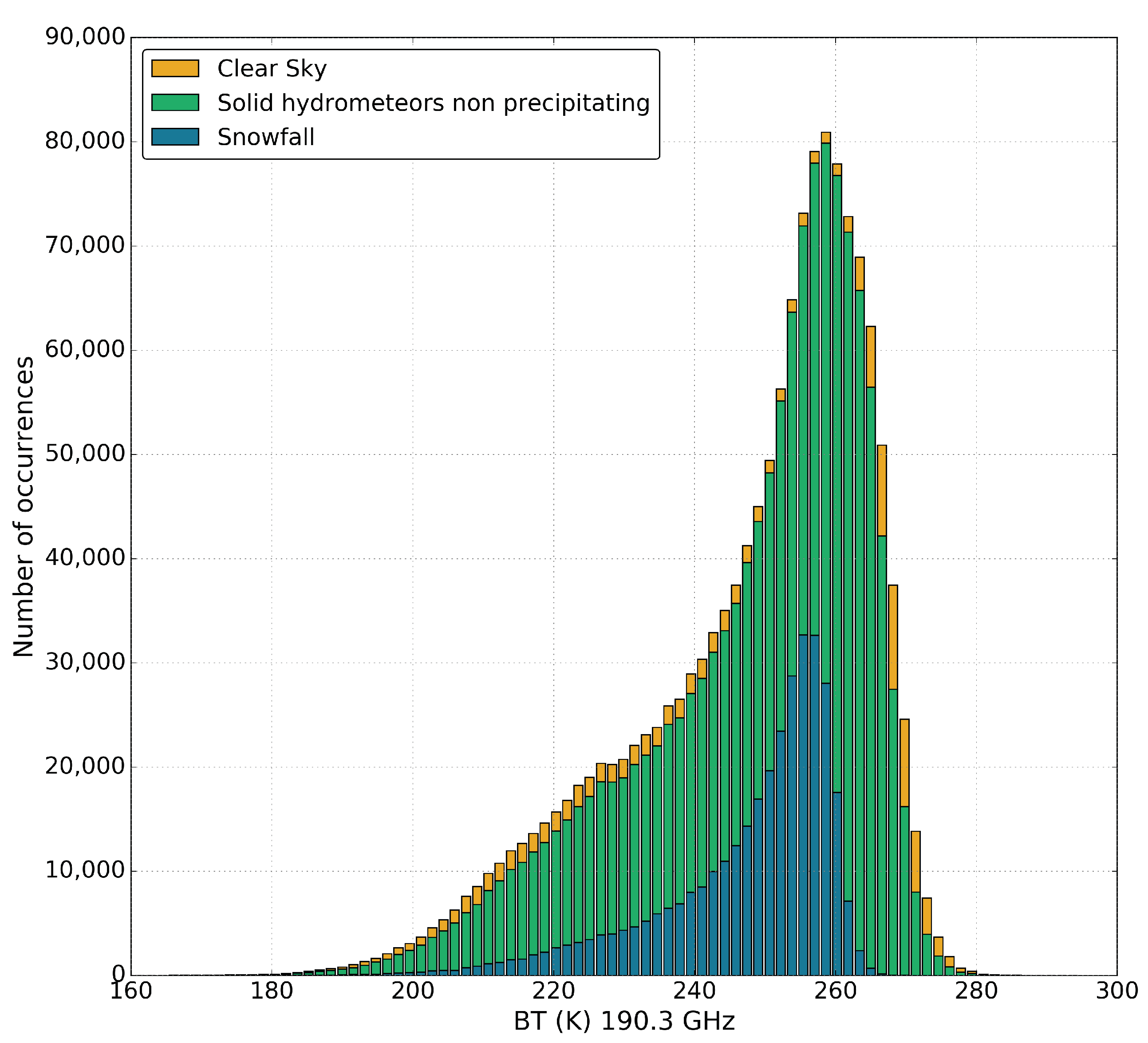
First, we tried to detect a systematic BT signature associated with snowfall events using a threshold approach. The BT distribution as a function of the type of event was computed for Channel 3 (Figure 3). BT overlaps exist between all types of events, indicating that it is impossible to distinguish snowfall cases from non-snowfall cases using a simple threshold method. The same behavior was observed at the other MHS frequencies. The snowfall signal is unclear because BT combines the impacts of both the surface and the atmosphere. The snowfall cases presented in the next section help reveal the different contributions from these impacts and the snowfall to the BT.
3.1. Arctic Case Studies
3.1.1. 30 November 2007 over Siberia
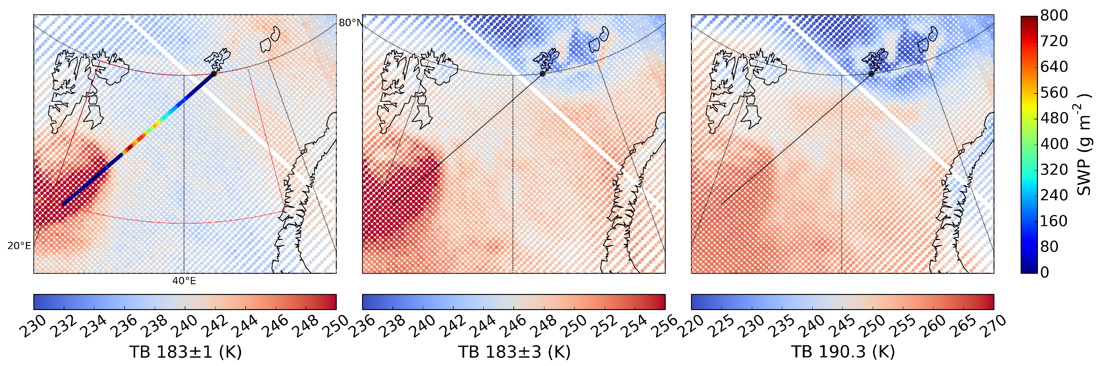
The first case took place on 30 November 2007 over sea ice in northern Siberia. CloudSat cross-section and co-located MHS measurements are plotted in Figure 4. The upper panel presents vertical profiles of the snowfall rates retrieved by 2C-SP, and the lower panel presents the co-located MHS BT measured at high frequencies. The red line in the upper panel represents the integrated water vapor (IWV). The maximum snowfall rate reached 2.5 mm h−1 at approximately 4 km, and the snowfall was very weak up to 10 km. During this event, IWV ranged from 12 kg m−2–14 kg m−2. A strong BT decrease of approximately 15 K was observed at 190.3 GHz, as well as a smaller decrease of approximately 5 K at 183.3 ± 3 GHz. This signal is due to scattering by solid hydrometeors. In Figure 5, the full-swath BT measurements are shown at the MHS frequencies near 183.3 GHz with the snow water path (SWP) indicated along the CloudSat track in the left panel. Along the CloudSat track, the BT is at a local minimum when SWP is at a local maximum. Interestingly, no signal was noted at 183.3 ± 1 GHz, which may sound too high into the atmosphere, i.e., above the altitude of high snowfall rates.
3.1.2. 29 March 2007 over the Barents Sea
The second snowfall event occurred on 29 March 2007 over the Barents Sea and is plotted in Figure 6. The cloud top height reached approximately 8 km, and the maximum snowfall rates were located between 2 km and 4 km with values of up to 2 mm h−1.
As shown in the upper panel of Figure 6, IWV increased from 2 kg m−2–7 kg m−2 between 80°N 47°E and 77°N 30°E and stayed constant southward. Between 80°N and 78°N, the BT at 190.3 GHz increased from 230 K–250 K, following the atmospheric water vapor gradient. Note that SIC decreased between 79°N and 78°N, leaving an ice-free ocean to the south (not shown). From 78°N–76.4°N, the BT remained constant for all frequencies. Only slight variations in BT were observed at 190.3 GHz, close to the most intense snowfall rates. Southward of 76.4°N, the BT at all frequencies suddenly increased by ∼10–15 K. The spatial distribution of this increase can be distinctly observed southward of 76°N and westward of 30°E in Figure 7. This increase in BT was observed for all three frequencies around 183 GHz, which indicates that this wetter air mass was vertically expanded and experienced an abrupt change in SWP, as highlighted by the CloudSat 2C-SP track.
Unlike the first snowfall event, no significant BT decrease was observed in the presence of snowfall. Note the stable BT between 78°N and 76.4°N and the sudden increase in BT at lower latitudes. A likely explanation for this is that the PMW measurements were masked due to the surface temperature from the open ocean between 78°N and 76.4°N, which is warmer than that of sea ice. The distinct BT increase took place where the snowfall stops while above open water. In the northern part of this event (north of 79.3°N, left of the figure), the lower BT at 190 GHz than at 183.3 ± 3 GHz and 183.3 ± 1 GHz was likely due to a partial contamination from the frozen ground related to the low humidity.
These two examples illustrate two typical snowfall situations in the Arctic. Analyzing the environmental conditions, we recorded a decrease in the BT due to scattering by snowflakes and no BT modification due to the masking effect of emissions from a warmer surface. This highlights the strong need to take into account environmental conditions in association with the BT to detect snowfall in the Arctic. In the next section, using these results, we develop a snowfall detection algorithm using the important environmental variables.
3.2. Snowfall Detection Algorithm
An RF method [44] was used to create a snowfall detection algorithm. In our case, RF returns a statistical probability of snowfall depending on the input variables. The following nine variables were provided to the RF: BT for all frequencies, IWV (kg m−2), the temperature at 2 m above the ground (T2m, K), the surface type (ST), and SIC. All integrated variables were considered between 12,000 m and the CPR near-surface bin height, that is ∼500 or 1000 m above oceans or continents, respectively.
First, we evaluate the RF performance for predicting snowfall events. Then, we present a single decision tree to analyze the variable selection used in RF. The environmental variables and associated thresholds that most effectively split the dataset between snowfall and non-snowfall profiles are then interpreted to understand the processes operating inside the snowfall detection algorithm.
3.2.1. Snowfall Prediction Performances
In this section, RF is used to predict the class of each pixel. To do so, our dataset was randomly split into training and test datasets, containing 80% and 20%, respectively, of all the profiles. The training dataset was used to train the RF, and then, the trained algorithm was applied to the test dataset to evaluate its performance. The RF algorithm was run with the number of trees ranging from 1–300. We chose to use 100 trees because this number of trees yields the best performance, and no significant improvements appeared when adding more trees. Results from this evaluation are presented below.
In Table 3, the confusion matrix for the test profiles from RF shows a similar proportion of false negatives (10.2% of all profiles, 14% of non-snowfall profiles) and false positives (8.7% of all profiles, 34% of snowfall profiles). The probability of detection (POD) was approximately 0.62; the false alarm rate was 0.34; and the Heidke skill score (HSS) was 0.51. An HSS of 0.51 can be interpreted as 51% of the correct classification not being due to chance, and the POD of 0.62 testifies to the good snowfall detection capability of our algorithm.
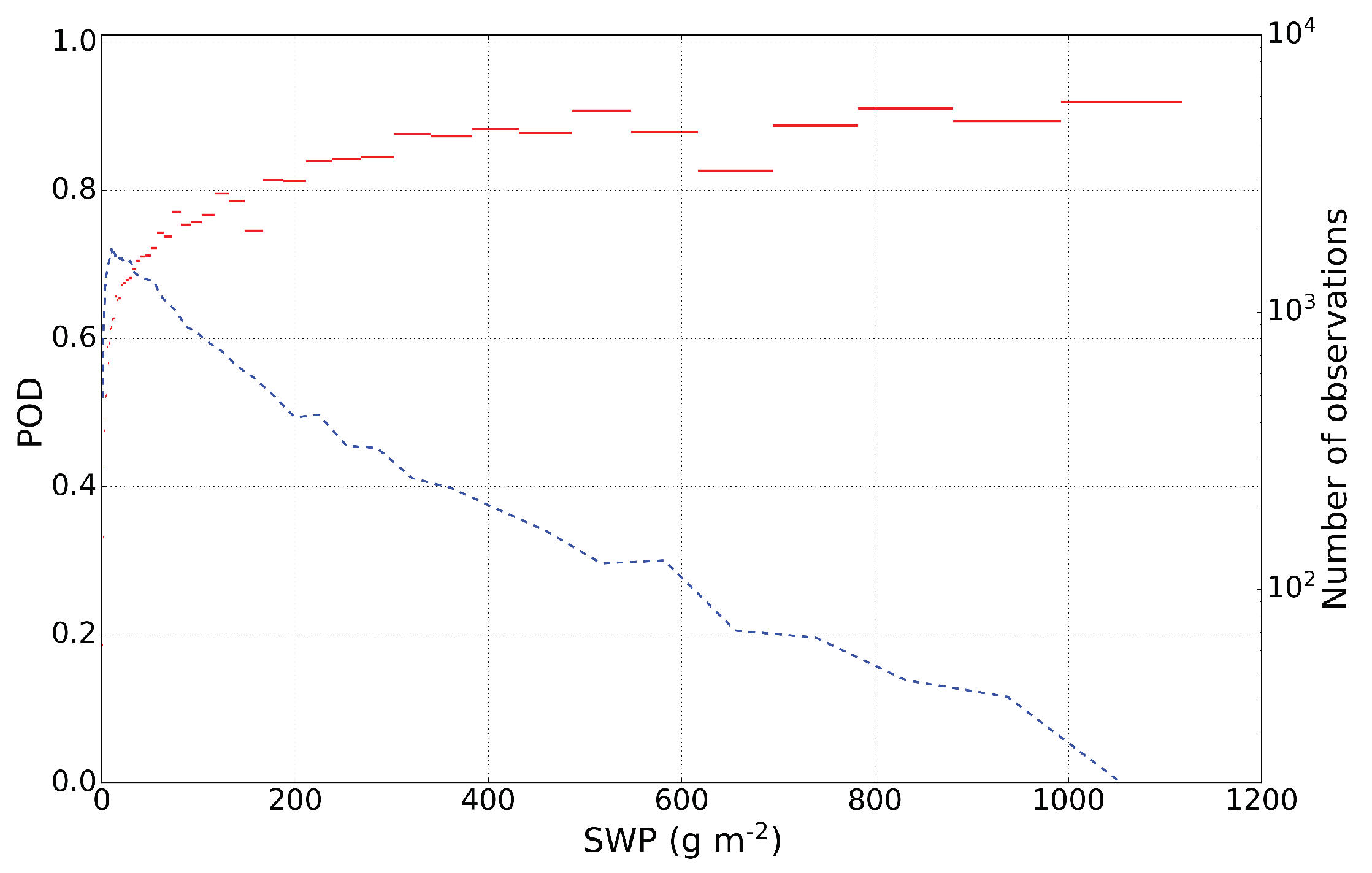
Here, the SWP value used to identify snowfall events in the CPR-MHS dataset was employed to evaluate the detection skill of the algorithm. As can be seen in Figure 8, POD increased with SWP; it exceeded 0.8 from approximately 200 g m−2 and reached 0.9 above 400 g m−2. However, note that SWP in the coincident database had a range of 0–1000 g m−2 with 90% of all profiles below 220 g m−2. This result demonstrates that the RF algorithm had a greater ability to detect intense snowfall than weak snowfall events.
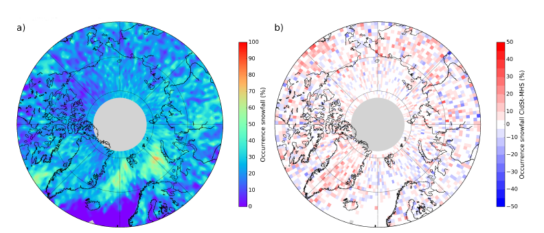
The snowfall occurrence from the MHS algorithm obtained for the test profiles is shown over a 1° latitude × 2° longitude grid in Figure 9a. The percentage of snowfall occurrence is defined as the number of algorithm-detected snowfall profiles divided by the total number of profiles. The highest snowfall occurrences were located in the Greenland and the Barents Seas (up to 80%), as well as in the Labrador Sea (southwest of Greenland, ∼60%) and central Siberia (∼50%). The snowfall occurrence differences between the test profiles from CloudSat and those from the MHS algorithm are plotted in Figure 9b and ranged between −25% and 30%, with the 25 and 75 percentiles at approximately −3% and 7%, respectively. The mean snowfall occurrence difference of 4% indicates a slightly higher snowfall occurrence observed by CloudSat than that retrieved by the MHS algorithm. Such a small difference is expected because RF was trained with the CloudSat dataset. While the snowfall occurrence differences were small over sea ice and the Arctic Ocean, these differences show high variability over continental areas. Further, the MHS algorithm tended to underestimate the snowfall occurrence compared to CloudSat over the Greenland ice sheet and the Alaska Range (by as much as −30%), likely due to the extreme dryness of these areas. Meanwhile, the algorithm overestimated the snowfall occurrence over the North Atlantic (by up to 30%), likely due to the occurrence of mixed phase precipitation. As a consequence, the mean snowfall occurrences need to be interpreted with caution in these regions.
3.2.2. Importance of the Variables
The snowfall detection capability of the RF algorithm was evaluated in the previous section. In this section, we analyze the importance of the variables as provided by the RF algorithm, and then, this information is interpreted using a decision tree with the same input variables.
The importance of each variable is shown in Table 4. The most important variable for snowfall detection was BT for Channel 5 (ch5), T2m, IWV, and Channel 4 (ch4) with a relative importance between 0.20 and 0.13. All variables made a significant contribution, except SIC and ST (≤0.04).
A decision tree was provided with the same input variables as the snowfall detection algorithm based on the RF algorithm to better understand how RF uses the input variables to classify snowfall and non-snowfall events. This tree appears similar to those generated by the RF algorithm. The structure of the tree (Figure 10a) illustrates the hierarchical selection operated by the tree, highlighting the variables and thresholds that most effectively split the dataset. The final subsets are defined by the conditions indicated for each input variable selected by the tree (for each split). Note that the tree expansion was statistically limited to keep only the most relevant split; if a node did not lead to a minimum improvement in the classification, then the split was not made, and the profiles in the node were considered to be a final subset. As a consequence, the variables selected were also limited and may not accurately reflect the importance reported by the snowfall detection algorithm. This point is further discussed later in this section.
The nodes and their physical meanings are explained below. The first node (ch5 ≤ 261 K) showed that a low BT most effectively split the initial dataset between snowfall and no-snowfall cases. A low BT may occur when hydrometeors scatter the signal or if the frequency measures emissions from the frozen ground. The second node (Channel 2 (ch2) ≥ 216 K) was associated with the environmental conditions and can be explained as follows. As stated in Section 2, the channel at 157 GHz is primarily used to quantify water vapor and probes close to the ground (Figure 1). Both the atmosphere and the surface contribute to these measurements. Therefore, low values of ch2 likely correspond to contamination of the BT by emission from the frozen ground, which is linked to the low temperature at the ground and the humidity, while high values likely correspond to a warmer and wetter atmosphere with a reduced contribution from the surface emission. Most of the profiles with ch2 values below the selected threshold occurred in a sufficiently cold and dry atmosphere to also contaminate the signal at frequencies near 183 GHz and, therefore, were excluded. However, the decision tree may remove some of the intense snowfall rate cases that induce a strong BT decrease in ch5 compared to that in ch4. The third node (ch4 ≤ 251 K) expressed the same type of condition as the first node but for Channel 4. The last node (T2m ≥ 262 K) is a necessary condition to ensure that the temperature (related to the maximum water vapor capacity of the air) is high enough to avoid ground contamination. Even though this was partially achieved by the second node (ch2), T2m was still an effective variable to split the dataset between snowfall and non-snowfall profiles with similar environmental conditions and BTs. Note that the thresholds yielded by the tree were indicative, meaning that most, but not all of the snowfall profiles occurred under the expressed conditions (i.e., some profiles with T2m ≥ 262 K might still be affected by ground emissions). When the following conditions are met: ch5 ≤ 261 K, ch2 ≥ 216 K, ch4 ≤ 251 K, and T2m ≥ 262 K, this decision tree classifies a pixel as having snowfall because there was statistically more snowfall than non-snowfall profiles (58%) in this subset (hereafter called the “snowfall subset”). Two major differences can be noted with respect to the importance of RF. First, the IWV importance was relatively high (0.16) in the RF algorithm; however, IWV was not selected by the single decision tree due to the limited tree expansion. Indeed, IWV and T2m are closely related in the atmosphere, meaning that using both variables may lead to redundant information. Therefore, to avoid increasing the complexity without improving the classification, IWV was not used in this tree configuration. Second, ch2 BT was considered to be more important in the single decision tree than in RF. The low values of ch2 correspond to the contamination of the BT by emission from the frozen ground, which is linked to the low temperature at the ground and the humidity. However, ch2 BT may be impacted by other variables (e.g., droplets or cloud ice), while T2m and IWV characterize the atmospheric state more precisely. Therefore, they were more indicative in the RF algorithm, which is more precise than the single decision tree due to its multiple fully-grown decision trees.
Note that the profiles inside the snowfall subset are not restricted to a specific area or season, but are well distributed both spatially and temporally. In Figure 10b, the proportion of snowfall cases over sea ice, oceans, and continents for each season with respect to the total number of snowfall cases is presented. The highest proportions of snowfall cases were observed in autumn above sea ice, continents, and the open ocean with values of 0.39, 0.36, and 0.29, respectively. In spring and summer, similar proportions were observed over sea ice (∼0.27) and continents (∼0.22). In winter, proportions of 0.11 and 0.09 were observed above sea ice and continents, respectively. Over the open ocean, proportions of approximately 0.33 were observed in winter and spring, while in summer, this proportion was approximately 0.17. This spatial and temporal distribution can be attributed to the fact that these environmental conditions for snowfall detection were more likely to occur in autumn and spring than in other seasons. Indeed, the humidity can be high; the temperature was not yet (or no longer) too low; and intense snowfall events can occur. The 58% of snowfall profiles in the snowfall subset corresponded to ∼27% of all the snowfall profiles and represented ∼51% of the total SWP.
This expansion-limited tree was employed as a tool to identify the conditions for which snowfall can statistically be detected. The interpretation of these conditions and their physical meanings, accordingly, allow a better understanding of the hierarchical variable selection that takes place in RF. The next section discusses the advantages and limitations of the snowfall detection algorithm.
4. Discussion
The advantages of the present detection algorithm are discussed below. The large 2180-km swath of microwave sounders enabled better spatial and temporal coverage compared to active microwave measurements. Moreover, the MHS design and measurements were similar to those of AMSU-B with only minor frequency changes. Both MHS and AMSU-B are included on board several satellites from the National Oceanic and Atmospheric Administration (NOAA) and the European Organisation for the Exploitation of Meteorological Satellites (EUMETSAT) associated with the European Space Agency (ESA). Therefore, MHS-type measurements began in 1999 on NOAA-15 and are still on going aboard Metop-C. This study encourages their use in geo-observing and future space missions, such as EarthCARE, to ensure the continuity of such measurements. The 20-year-long time series and the increased amount of data compared to CloudSat represent clear advantages for precipitation characterization because fewer events are likely to be missed, and measurements are available up to 90°N.
Our approach does present some limitations. One limitation concerns the CloudSat products. Even though these products have been evaluated against various observations and datasets and have shown good agreement (e.g., [46,47]), uncertainties remain, especially due to ground clutter and the CloudSat blind zone. Further, instrument characteristics and algorithm assumptions may lead to significant differences with respect to other satellite-based snowfall products [48]. The consequent snowfall detection errors from CloudSat would impact the performance of the MHS algorithm. Moreover, due to the finer horizontal resolution of CPR, several CPR profiles were averaged over each MHS measurement. Over one MHS pixel, multiple CloudSat profiles can indicate different precipitation flags detected by 2C-PC, and several methods can be considered to address this issue. We removed the ambiguous profiles to minimize the initial uncertainties in our dataset. Regression trees and RF are sensitive to the training dataset, which necessitates caution when interpreting the results, particularly the threshold values. Moreover, by definition, RF cannot extrapolate outside its training data. Using two years of co-located observations, we were able to sample a large range of snowfall events. However, extreme events outside our spectrum of observation remain possible. In addition, the snowfall detection algorithm depends on IWV and T2m, which are obtained from ERA-Interim. T2m tends to have a warm bias when compared to Arctic buoy observations, which is more pronounced in the winter months [49]. ERA-Interim is also known to be drier than most reanalyzes [50,51], especially regarding snowfall, which may be related to its high rainfall to precipitation ratio. Even though most favorable cases for snowfall detection are likely to be in a mild and wet environment, the snowfall detection might be affected by a low temperature bias. Therefore, sensitivity tests to errors in T2m and IWV need to be conducted.
Other reanalyzes could also be used, such as ERA5 or the Arctic System Reanalysis, which exhibit T2m and IWV values closer to those of polar station measurements than the ERA-Interim values [52]. In this study, we focused on passive instrument angles of less than 15°. As we approach the edge of the swath, the MHS pixel size increases up to 26 km × 50 km, whereas the CloudSat footprint (1.7 km × 1.4 km) remains unchanged. Using remote sensing observations with high horizontal resolution differences may be inappropriate. Moreover, the BT varies as a function of the angle due to the polarization and the path into the atmosphere. Skofronick-Jackson and Johnson [19] reported that, depending on the snowfall event, the hydrometeor contribution to the BT can increase significantly at an angle of 53° compared to at nadir. Further studies are needed to investigate whether large angles can also be considered. Finally, the impact of supercooled water on the BT needs to be investigated because it may mask the snowfall signal due to emission from liquid water [20,24,25]. This is a rather common phenomenon in the Arctic and requires additional research.
5. Conclusions
The aim of our study was to assess the potential use of PMW observations for detecting snowfall at Arctic latitudes. Innovative methods (the random forest (RF) classifier and decision trees) were used to obtain the following main results.
- We developed an algorithm using MHS observations and environmental variables to detect snowfall in the Arctic. This algorithm attests to the importance of the near surface temperature and the brightness temperature (BT) at 190.3 GHz and 183.3 ± 3 GHz and highlights the importance of IWV for snowfall detection. Unlike lower latitude studies, measurements at 190.3 GHz and 183.3 ± 3 GHz were found to capture most of the scattering signatures under Arctic conditions, while commonly-used frequencies (e.g., 157 GHz) contained nearly no information concerning snowfall detection.
- The overall probability of detection (POD) was close to 0.62 and was between 0.8 and 0.9 for profiles above 200 g m−2, which indicates that the algorithm performs better for intense snowfall events than for weak snowfall events. However, POD did not reach one, meaning that the snowfall detection was not statistically certain, even for the most intense events, which could imply further difficulties for snowfall quantification. For the ∼200,000 test profiles, the algorithm yielded 10.2% false negatives and 8.7% false positives.
- Snowfall occurrence differences between CloudSat and the RF algorithm using MHS observations were computed. On average, the snowfall occurrence of CloudSat was 4% higher than that of MHS. These differences were up to 30% over Greenland and the Alaska Range likely due to the dryness of these areas and were as much as −30% over the North Atlantic likely due to the occurrence of mixed phase precipitation.
- The hierarchical variable selection in the snowfall detection algorithm, based on RF, was interpreted using a single decision tree as an analyzing tool. This expansion-limited tree identified the most important conditions for which snowfall could be statistically detected as being the scattering by snowflakes and a humid and mild troposphere. The interpretation of these conditions allowed the selection made by the RF algorithm to be better understood.
- Future studies should investigate the sensitivity of the BT to snowfall rates in order to develop a snowfall quantification algorithm in the Arctic.
Author Contributions
L.E. created the database, analyzed the cases, developed the random forest algorithm, and wrote this paper. J.-F.R. and C.C. supervised the study and closely followed the writing of the final draft. All co-authors contributed to the discussion of the results and to the improvement of the final draft.
Funding
This study was supported by the National French Research Agency (ANR) program AC-AHC2 (Circulation Atmospheric and Hydrological Cycle Changes in the Arctic), Number ANR-15-CE01-0015. This work was partially supported by the National Centre of Spatial Studies (CNES) program EECLAT (Expecting Earth-Care, Learning from A-Train). C.C., C.G., and C.P. acknowledge support from the ANR program APRES3, Number ANR-15-CE01-0003.
Acknowledgments
CloudSat data were obtained from the CloudSat Data Processing Center (http://www.cloudsat.cira.colostate.edu). We thank N. B. Wood and T. L’Ecuyer at the University of Wisconsin-Madison for valuable discussions regarding the CloudSat products. To process the MHS and CloudSat data, this study benefited from the IPSL (Institute Pierre Simon Laplace) Mesocentre ESPRI facility, which is supported by CNRS, UPMC (University Pierre and Marie Curie), Labex L-IPSL, CNES, and Ecole Polytechnique. We also thank AERIS (French Data Infrastructure for the Atmosphere) for access to the MHS data, ICARE for access to the DARDAR data, and the National Snow and Ice Data Center for access to the AMSR-E data (https://nsidc.org/data/au_si12/versions/1). We would also like to thank the three anonymous reviewers for their comments, which greatly improved the manuscript.
Conflicts of Interest
The funders had no role in the design of the study; in the collection, analyzes, or interpretation of data; in the writing of the manuscript; nor in the decision to publish the results.
References
- Hartmann, D.L.; Tank, A.M.K.; Rusticucci, M.; Alexander, L.V.; Brönnimann, S.; Charabi, Y.A.R.; Dentener, F.J.; Dlugokencky, E.J.; Easterling, D.R.; Kaplan, A.; et al. Observations: Atmosphere and surface. In Climate Change 2013 the Physical Science Basis: Working Group I Contribution to the Fifth Assessment Report of the Intergovernmental Panel on Climate Change; Cambridge University Press: Cambridge, UK, 2013. [Google Scholar]
- Vihma, T.; Screen, J.; Tjernström, M.; Newton, B.; Zhang, X.; Popova, V.; Deser, C.; Holland, M.; Prowse, T. The atmospheric role in the Arctic water cycle: A review on processes, past and future changes, and their impacts. J. Geophys. Res. Biogeosci. 2016, 121, 586–620. [Google Scholar] [CrossRef] [Green Version]
- Liu, Y.; Key, J.R.; Liu, Z.; Wang, X.; Vavrus, S.J. A cloudier Arctic expected with diminishing sea ice. Geophys. Res. Lett. 2012, 39. [Google Scholar] [CrossRef]
- Goodison, B.E.; Louie, P.Y.; Yang, D. WMO Solid Precipitation Measurement Intercomparison; World Meteorological Organization: Geneva, Switzerland, 1998. [Google Scholar]
- Nitu, R.; Roulet, Y.A.; Wolff, M.; Earle, M.; Reverdin, A.; Smith, C.; Kochendorfer, J.; Morin, S.; Rasmussen, R.; Wong, K.; et al. WMO Solid Precipitation Intercomparison Experiment (SPICE) (2012–2015); IOM No.131; World Meteorological Organization: Geneva, Switzerland, 2018. [Google Scholar]
- Candlish, L.M.; Raddatz, R.L.; Asplin, M.G.; Barber, D.G. Atmospheric temperature and absolute humidity profiles over the Beaufort Sea and Amundsen Gulf from a microwave radiometer. J. Atmos. Ocean. Technol. 2012, 29, 1182–1201. [Google Scholar] [CrossRef]
- Liu, G. Deriving snow cloud characteristics from CloudSat observations. J. Geophys. Res. Atmos. 2008, 113. [Google Scholar] [CrossRef] [Green Version]
- Haynes, J.M.; L’Ecuyer, T.S.; Stephens, G.L.; Miller, S.D.; Mitrescu, C.; Wood, N.B.; Tanelli, S. Rainfall retrieval over the ocean with spaceborne W-band radar. J. Geophys. Res. Atmos. 2009, 114. [Google Scholar] [CrossRef]
- Wood, N.B.; L’Ecuyer, T.S.; Heymsfield, A.J.; Stephens, G.L.; Hudak, D.R.; Rodriguez, P. Estimating snow microphysical properties using collocated multisensor observations. J. Geophys. Res. Atmos. 2014, 119, 8941–8961. [Google Scholar] [CrossRef]
- Seto, S.; Takahashi, N.; Iguchi, T. Rain/no-rain classification methods for microwave radiometer observations over land using statistical information for brightness temperatures under no-rain conditions. J. Appl. Meteorol. 2005, 44, 1243–1259. [Google Scholar] [CrossRef]
- Prigent, C. Precipitation retrieval from space: An overview. C. R. Geosci. 2010, 342, 380–389. [Google Scholar] [CrossRef]
- Kidd, C.; Levizzani, V. Status of satellite precipitation retrievals. Hydrol. Earth Syst. Sci. 2011, 15, 1109–1116. [Google Scholar] [CrossRef] [Green Version]
- Maggioni, V.; Meyers, P.C.; Robinson, M.D. A review of merged high-resolution satellite precipitation product accuracy during the Tropical Rainfall Measuring Mission (TRMM) era. J. Hydrometeorol. 2016, 17, 1101–1117. [Google Scholar] [CrossRef]
- Levizzani, V.; Laviola, S.; Cattani, E. Detection and measurement of snowfall from space. Remote Sens. 2011, 3, 145–166. [Google Scholar] [CrossRef]
- Kongoli, C.; Meng, H.; Dong, J.; Ferraro, R. A hybrid snowfall detection method from satellite passive microwave measurements and global forecast weather models. Q. J. R. Meteorol. Soc. 2018, 144, 120–132. [Google Scholar] [CrossRef] [Green Version]
- Katsumata, M.; Uyeda, H.; Iwanami, K.; Liu, G. The response of 36-and 89-GHz microwave channels to convective snow clouds over ocean: Observation and modeling. J. Appl. Meteorol. 2000, 39, 2322–2335. [Google Scholar] [CrossRef]
- Bennartz, R.; Bauer, P. Sensitivity of microwave radiances at 85–183 GHz to precipitating ice particles. Radio Sci. 2003, 38. [Google Scholar] [CrossRef]
- Noh, Y.J.; Liu, G. Satellite and aircraft observations of snowfall signature at microwave frequencies. Riv. Ital. Telerilevamento 2004, 30, 101–118. [Google Scholar]
- Skofronick-Jackson, G.; Johnson, B.T. Surface and atmospheric contributions to passive microwave brightness temperatures for falling snow events. J. Geophys. Res. Atmos. 2011, 116. [Google Scholar] [CrossRef]
- Panegrossi, G.; Rysman, J.F.; Casella, D.; Marra, A.; Sanò, P.; Kulie, M. CloudSat-based assessment of GPM Microwave Imager snowfall observation capabilities. Remote. Sens. 2017, 9, 1263. [Google Scholar] [CrossRef]
- Noh, Y.J.; Liu, G.; Jones, A.S.; Vonder Haar, T.H. Toward snowfall retrieval over land by combining satellite and in situ measurements. J. Geophys. Res. Atmos. 2009, 114. [Google Scholar] [CrossRef]
- Liu, G.; Seo, E.K. Detecting snowfall over land by satellite high-frequency microwave observations: The lack of scattering signature and a statistical approach. J. Geophys. Res. Atmos. 2013, 118, 1376–1387. [Google Scholar] [CrossRef]
- Liu, G. A database of microwave single-scattering properties for nonspherical ice particles. Bull. Am. Meteorol. Soc. 2008, 89, 1563–1570. [Google Scholar] [CrossRef]
- Kneifel, S.; Löhnert, U.; Battaglia, A.; Crewell, S.; Siebler, D. Snow scattering signals in ground-based passive microwave radiometer measurements. J. Geophys. Res. Atmos. 2010, 115. [Google Scholar] [CrossRef] [Green Version]
- Xie, X.; Löhnert, U.; Kneifel, S.; Crewell, S. Snow particle orientation observed by ground-based microwave radiometry. J. Geophys. Res. Atmos. 2012, 117. [Google Scholar] [CrossRef]
- Wang, Y.; Liu, G.; Seo, E.K.; Fu, Y. Liquid water in snowing clouds: Implications for satellite remote sensing of snowfall. Atmos. Res. 2013, 131, 60–72. [Google Scholar] [CrossRef]
- You, Y.; Wang, N.Y.; Ferraro, R.; Rudlosky, S. Quantifying the snowfall detection performance of the GPM microwave imager channels over land. J. Hydrometeorol. 2017, 18, 729–751. [Google Scholar] [CrossRef]
- Rysman, J.F.; Panegrossi, G.; Sanò, P.; Marra, A.; Dietrich, S.; Milani, L.; Kulie, M. SLALOM: An all-surface snow water path retrieval algorithm for the GPM Microwave Imager. Remote Sens. 2018, 10, 1278. [Google Scholar] [CrossRef]
- You, Y.; Wang, N.Y.; Ferraro, R. A prototype precipitation retrieval algorithm over land using passive microwave observations stratified by surface condition and precipitation vertical structure. J. Geophys. Res. Atmos. 2015, 120, 5295–5315. [Google Scholar] [CrossRef]
- Kulie, M.S.; Milani, L.; Wood, N.B.; Tushaus, S.A.; Bennartz, R.; L’Ecuyer, T.S. A shallow cumuliform snowfall census using spaceborne radar. J. Hydrometeorol. 2016, 17, 1261–1279. [Google Scholar] [CrossRef]
- Skofronick-Jackson, G.M.; Johnson, B.T.; Munchak, S.J. Detection thresholds of falling snow from satellite-borne active and passive sensors. IEEE Trans. Geosci. Remote Sens. 2013, 51, 4177–4189. [Google Scholar] [CrossRef]
- Kongoli, C.; Meng, H.; Dong, J.; Ferraro, R. A snowfall detection algorithm over land utilizing high-frequency passive microwave measurements-Application to ATMS. J. Geophys. Res. Atmos. 2015, 120, 1918–1932. [Google Scholar] [CrossRef]
- Surussavadee, C.; Staelin, D.H. Satellite retrievals of arctic and equatorial rain and snowfall rates using millimeter wavelengths. IEEE Trans. Geosci. Remote Sens. 2009, 47, 3697–3707. [Google Scholar] [CrossRef]
- Melsheimer, C.; Heygster, G. Improved retrieval of total water vapor over polar regions from AMSU-B microwave radiometer data. IEEE Trans. Geosci. Remote Sens. 2008, 46, 2307–2322. [Google Scholar] [CrossRef]
- Grody, N.; Weng, F.; Ferraro, R. Application of AMSU for obtaining hydrological parameters. In Microwave Radiometry and Remote Sensing of the Earth’s Surface and Atmosphere; VSP: Zeist, The Netherlands, 2000; pp. 339–352. [Google Scholar]
- Saunders, R.; Hocking, J.; Turner, E.; Rayer, P.; Rundle, D.; Brunel, P.; Vidot, J.; Roquet, P.; Matricardi, M.; Geer, A.; et al. An update on the RTTOV fast radiative transfer model (currently at version 12). Geosci. Model Dev. 2018, 11, 2717–2737. [Google Scholar] [CrossRef] [Green Version]
- Milani, L.; Kulie, M.S.; Casella, D.; Dietrich, S.; L’Ecuyer, T.S.; Panegrossi, G.; Porcù, F.; Sanò, P.; Wood, N.B. CloudSat snowfall estimates over Antarctica and the Southern Ocean: An assessment of independent retrieval methodologies and multi-year snowfall analysis. Atmos. Res. 2018, 213, 121–135. [Google Scholar] [CrossRef]
- Palerme, C.; Claud, C.; Wood, N.; L’Ecuyer, T.; Genthon, C. How does ground clutter affect CloudSat snowfall retrievals over ice sheets? IEEE Geosci. Remote. Sens. Lett. 2019, 16, 342–346. [Google Scholar] [CrossRef]
- Delanoë, J.; Hogan, R.J. Combined CloudSat-CALIPSO-MODIS retrievals of the properties of ice clouds. J. Geophys. Res. Atmos. 2010, 115. [Google Scholar] [CrossRef] [Green Version]
- Cronk, H.; Partain, P. CloudSat ECMWF-AUX Auxillary Data Product Process Description and Interface Control Document, Product Version P R05. NASA JPL CloudSat project document revision 0. 2017, p. 15. Available online: http://www.cloudsat.cira.colostate.edu/data-products/level-aux/ecmwf-aux?term=85 (accessed on 19 September 2019).
- Cavalieri, D.J.; Markus, T.; Comiso, J.C. AMSR-E/Aqua Daily L3 12.5 km Brightness Temperature, Sea Ice Concentration, & Snow Depth Polar Grids, Version 3; NASA National Snow and Ice Data Center Distributed Active Archive Center: Boulder, CO, USA, 2014. [Google Scholar] [CrossRef]
- EUMETSAT. ATOVS Level 1b Product Guide. EUMETSAT, Document Revision 3. 2010, p. 202. Available online: http://www.eumetsat.int/website/wcm/idc/idcplg?IdcService=GET_FILE&dDocName=pdf_v2a_atovs_level_1b&RevisionSelectionMethod=LatestReleased&Rendition=Web (accessed on 19 September 2019).
- Breiman, L.; Friedman, J.; Olshen, R.; Stone, C. Classification and regression trees. Wadsworth Int. Group 1984, 37, 237–251. [Google Scholar]
- Breiman, L. Random forests. Mach. Learn. 2001, 45, 5–32. [Google Scholar] [CrossRef]
- Hastie, T.; Tibshirani, R.; Friedman, J.; Franklin, J. The elements of statistical learning: Data mining, inference and prediction. Math. Intell. 2005, 27, 83–85. [Google Scholar]
- Norin, L.; Devasthale, A.; L’Ecuyer, T.; Wood, N.; Smalley, M. Intercomparison of snowfall estimates derived from the CloudSat Cloud Profiling Radar and the ground-based weather radar network over Sweden. Atmos. Meas. Tech. 2015, 8, 5009–5021. [Google Scholar] [CrossRef] [Green Version]
- Chen, S.; Hong, Y.; Kulie, M.; Behrangi, A.; Stepanian, P.M.; Cao, Q.; You, Y.; Zhang, J.; Hu, J.; Zhang, X. Comparison of snowfall estimates from the NASA CloudSat cloud profiling radar and NOAA/NSSL multi-radar multi-sensor system. J. Hydrol. 2016, 541, 862–872. [Google Scholar] [CrossRef]
- Skofronick-Jackson, G.; Kulie, M.; Milani, L.; Munchak, S.J.; Wood, N.B.; Levizzani, V. Satellite estimation of falling snow: A global precipitation measurement (GPM) core observatory perspective. J. Appl. Meteorol. Climatol. 2019, 58, 1429–1448. [Google Scholar] [CrossRef]
- Wang, C.; Graham, R.M.; Wang, K.; Gerland, S.; Granskog, M.A. Comparison of ERA5 and ERA-Interim near surface air temperature and precipitation over Arctic sea ice: Effects on sea ice thermodynamics and evolution. Cryosphere 2018, 13, 1661–1679. [Google Scholar] [CrossRef]
- Boisvert, L.N.; Webster, M.A.; Petty, A.A.; Markus, T.; Bromwich, D.H.; Cullather, R.I. Intercomparison of precipitation estimates over the Arctic Ocean and its peripheral seas from reanalyzes. J. Clim. 2018, 31, 8441–8462. [Google Scholar] [CrossRef]
- Palerme, C.; Claud, C.; Dufour, A.; Genthon, C.; Wood, N.B.; L’Ecuyer, T. Evaluation of Antarctic snowfall in global meteorological reanalyzes. Atmos. Res. 2017, 190, 104–112. [Google Scholar] [CrossRef]
- Bromwich, D.H.; Wilson, A.B.; Bai, L.S.; Moore, G.W.; Bauer, P. A comparison of the regional Arctic System Reanalysis and the global ERA-Interim Reanalysis for the Arctic. Q. J. R. Meteorol. Soc. 2016, 142, 644–658. [Google Scholar] [CrossRef]
Figure 1.
Clear-sky weighting functions for the MHS channels for a polar atmosphere (over Svalbard) in (a) January and (b) July 2007. The weighting functions were calculated using RTTOV Version 12 for the nadir view and then smoothed with a polynomial function.
Figure 1.
Clear-sky weighting functions for the MHS channels for a polar atmosphere (over Svalbard) in (a) January and (b) July 2007. The weighting functions were calculated using RTTOV Version 12 for the nadir view and then smoothed with a polynomial function.

Figure 2.
Frequency as a function of latitude for different types of events detected for all profiles of the 2007–2008 Cloud Profiling Radar (CPR)-MHS dataset.
Figure 2.
Frequency as a function of latitude for different types of events detected for all profiles of the 2007–2008 Cloud Profiling Radar (CPR)-MHS dataset.

Figure 3.
Number of occurrences as a function of the BT (K) at 190.3 GHz for the different types of detected events.
Figure 3.
Number of occurrences as a function of the BT (K) at 190.3 GHz for the different types of detected events.

Figure 4.
Co-located observations of CloudSat and MHS (on NOAA-18) along the CloudSat track over a snowfall event located north of Siberia on 30 November 2007. (a) Snowfall rate profiles (mm h−1, left axis) from CloudSat 2C-SP. The red line corresponds to integrated water vapor (IWV) (kg m−2, right axis) from ECMWF-AUX. (b) Co-located BT (K) measurements from MHS for 183.3 ± 1 GHz, 183.3 ± 3 GHz, and 190.3 GHz.

Figure 5.
BT (K) measured by MHS for 183.3 ± 1 GHz, 183.3 ± 3 GHz, and 190.3 GHz (from left to right). The black line indicates the CloudSat overpass seen in Figure 4, while the black dot shows the beginning of the track. In the left panel, the CloudSat track shows snow water path (SWP) (g m−2).
Figure 5.
BT (K) measured by MHS for 183.3 ± 1 GHz, 183.3 ± 3 GHz, and 190.3 GHz (from left to right). The black line indicates the CloudSat overpass seen in Figure 4, while the black dot shows the beginning of the track. In the left panel, the CloudSat track shows snow water path (SWP) (g m−2).

Figure 6.
Same as Figure 4, but for the snowfall event located over the Barents Sea on 29 March 2007.
Figure 6.
Same as Figure 4, but for the snowfall event located over the Barents Sea on 29 March 2007.

Figure 7.
Same as Figure 5, but for the second snowfall case presented in Figure 6. The SWP color bar scale is different from that in Figure 5.

Figure 8.
Probability of detection (POD) as a function of SWP with logarithmically-scaled bins in red. The blue line corresponds to the number of observations in each bin plotted on a logarithmic axis.
Figure 8.
Probability of detection (POD) as a function of SWP with logarithmically-scaled bins in red. The blue line corresponds to the number of observations in each bin plotted on a logarithmic axis.

Figure 9.
(a) The snowfall occurrence obtained using the MHS algorithm. The snowfall occurrence is defined as the number of algorithm-detected snowfall profiles divided by the total number of profiles (%) over a 1° latitude × 2° longitude grid. Grey cells are plotted where no data are available. (b) Differences between the snowfall occurrence (%) of CloudSat and that retrieved (%) by the RF algorithm using MHS. Profiles from the testing dataset were used and represent 20% of the entire CPR-MHS dataset. Of the 210,891 profiles used, 56,668 were classified as snowfall profiles by CloudSat and 52,871 were classified as snowfall profiles by MHS.

Figure 10.
(a) Decision tree classifier with the environmental variables and BT as inputs. The percentage of the number of snowfall cases with respect to the total number of profiles is shown for each leaf node. Proportions greater than 50% are shown in green; otherwise, they are shown in red. (b) Proportion of snowfall events in the “snowfall group” with respect to the total number of snowfall events as a function of the season and the surface type.


Table 1.
Microwave Humidity Sounder (MHS) channels’ characteristics.
| Channel | Central Frequency (GHz) |
|---|---|
| 1 | 89.0 |
| 2 | 157.0 |
| 3 | 183.311 ± 1.0 |
| 4 | 183.311 ± 3.0 |
| 5 | 190.311 |
Table 2.
Summary of the products used in this study. AUX, auxiliary; AMSR-E, Advanced Microwave Scanning Radiometer for EOS.
Table 2.
Summary of the products used in this study. AUX, auxiliary; AMSR-E, Advanced Microwave Scanning Radiometer for EOS.
| Name | Main Variables | Reference |
|---|---|---|
| MHS | Brightness temperature (BT) | [42] |
| 2C-PRECIP-COLUMN | Occurrence, phase, and likelihood of precipitation | [8] |
| 2C-SNOW-PROFILE | Snowfall rates and snow water content | [9] |
| ECMWF-AUX | Temperature, pressure, and specific humidity | [40] |
| DARDARMASK | Cloud type and ice water content | [39] |
| AMSR-E L3 | Sea ice concentration | [41] |
Table 3.
Confusion matrix for the RF algorithm: total number of cases with the percentage values in parentheses.
Table 3.
Confusion matrix for the RF algorithm: total number of cases with the percentage values in parentheses.
| Predicted | Reference | |
|---|---|---|
| No Snowfall | Snowfall | |
| No snowfall | 136,016 (64.5%) | 21,503 (10.2%) |
| Snowfall | 18,316 (8.7%) | 35,056 (16.6%) |
Table 4.
Importance of each input variable given by the RF algorithm. Here, Channels 1–5 are denoted by “ch” plus the channel number.
Table 4.
Importance of each input variable given by the RF algorithm. Here, Channels 1–5 are denoted by “ch” plus the channel number.
| Variables | ch5 | T2m | IWV | ch4 | ch2 | ch3 | ch1 | SIC | ST |
|---|---|---|---|---|---|---|---|---|---|
| Importance | 0.20 | 0.19 | 0.16 | 0.13 | 0.10 | 0.09 | 0.08 | 0.04 | 0.02 |
© 2019 by the authors. Licensee MDPI, Basel, Switzerland. This article is an open access article distributed under the terms and conditions of the Creative Commons Attribution (CC BY) license (http://creativecommons.org/licenses/by/4.0/).
Share and Cite
MDPI and ACS Style
Edel, L.; Rysman, J.-F.; Claud, C.; Palerme, C.; Genthon, C. Potential of Passive Microwave around 183 GHz for Snowfall Detection in the Arctic. Remote Sens. 2019, 11, 2200. https://doi.org/10.3390/rs11192200
AMA Style
Edel L, Rysman J-F, Claud C, Palerme C, Genthon C. Potential of Passive Microwave around 183 GHz for Snowfall Detection in the Arctic. Remote Sensing. 2019; 11(19):2200. https://doi.org/10.3390/rs11192200
Chicago/Turabian StyleEdel, Léo, Jean-François Rysman, Chantal Claud, Cyril Palerme, and Christophe Genthon. 2019. "Potential of Passive Microwave around 183 GHz for Snowfall Detection in the Arctic" Remote Sensing 11, no. 19: 2200. https://doi.org/10.3390/rs11192200
Note that from the first issue of 2016, this journal uses article numbers instead of page numbers. See further details here.