MODIS Aqua Reflective Solar Band Calibration for NASA’s R2018 Ocean Color Products


1
Science Applications International Corp., Reston, VA 20190, USA
2
NASA Goddard Space Flight Center, Ocean Ecology Laboratory, Greenbelt, MD 20771, USA
*
Author to whom correspondence should be addressed.
Remote Sens. 2019, 11(19), 2187; https://doi.org/10.3390/rs11192187
Submission received: 9 August 2019
/
Revised: 10 September 2019
/
Accepted: 12 September 2019
/
Published: 20 September 2019
(This article belongs to the Special Issue Fiducial Reference Measurements for Satellite Ocean Colour)
Abstract
:Remote-sensing ocean color products have stringent requirements on radiometric calibration stability. To address a calibration deficiency in Moderate Resolution Imaging Spectroradiometer (MODIS) Aqua in recent years, the NASA Ocean Biology Processing Group (OBPG) developed a new calibration for reflective solar bands. Prior to the reprocessing of NASA’s ocean color products for 2018 (R2018), the OBPG MODIS products had been based on calibration provided by the MODIS Calibration Support Team (MCST). Several modifications were made to the MCST calibration approach to improve the calibration accuracy for ocean color products. These include (1) applying 936-nm detector normalization to solar diffuser stability monitor (SDSM) data to reduce coherent noise; (2) modeling solar diffuser (SD) degradation wavelength dependency to determine SD degradation in near-infrared and shortwave infrared wavelengths; (3) computing detector gains using SD screen-closed data to better match ocean radiance levels in all bands; (4) performing a simple atmospheric correction to reduce bidirectional reflectance distribution function (BRDF) effects in desert trends; (5) estimating and using modulated relative spectral response (RSR) impact on ocean data to adjust the calibration coefficients; (6) using smoothing to characterize the temporal change in calibration; and characterizing response versus scan angle (RVS) changes using 2nd-order polynomials to improve spatial/temporal calibration stability. Relative to the previous R2014 ocean color products, the R2018 calibration removed the suspect late-mission global trends in blue-band water-leaving reflectance and some anomalously large short-term variability (spikes) in the temporal trend of chlorophyll concentration. This paper will describe the OBPG calibration with a focus on the differences between the MCST and OBPG approaches.
Keywords:
satellite; calibration; solar diffusor; SDSM; desert trend; lunar calibration; RVS; MODIS; Aqua; ocean color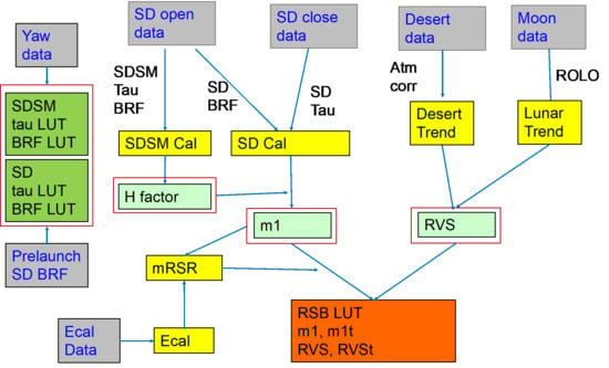
1. Introduction
The Moderate Resolution Imaging Spectroradiometer (MODIS) on the Earth Observing System (EOS) platform has 36 spectral bands to provide near-global observations every 2 days [1]. Of the 36 spectral bands, 20 are reflective solar bands (RSB) with a spectral range of 0.41 to 2.1 μm. Within the RSB, bands 8–16 are optimized to observe ocean biological processes (Table 1) and the rest of the RSB are designed for land and atmosphere applications but can also be used in ocean science application with reduced accuracy.
The MODIS is a key instrument aboard the Terra and Aqua Satellites. The two EOS spacecrafts, Terra and Aqua, were launched on 18 December 1999 and 4 May 2002, respectively, into sun-synchronous polar orbits at an altitude of 705 km. Terra is on a descending node with an equator crossing time of 10:30 AM (local time) and Aqua is on an ascending node with a 1:30 PM equator crossing time. Since they began operations, both instruments have continuously provided global earth observation data to study land, ocean, and atmospheric processes. However, due to the changing polarization sensitivities in MODIS Terra (MODIST) [2], the Terra ocean products have been relying on Ocean Biology Processing Group (OBPG) crosscalibration to correct the temporal calibration biases [3]. The crosscalibration uses MODIS Aqua (MODISA) global 7-day composites of water-leaving radiance as a truth field, combined with modeled atmospheric path radiance and surface contributions, to estimate the temporal change in gain and polarization as a function of time and scan angle.
Because of the MODIST-MODISA crosscalibration, the Terra ocean products are not considered an independent science data product and the accuracy of Terra products is dependent on the quality of Aqua products. Therefore, the calibration accuracy of MODISA is crucial, as the entire suite of MODIS ocean color products rely on the quality of Aqua products. Historically, the Aqua ocean color products are produced using the MODIS Calibration Support Team (MCST) radiometric calibration and are fine-tuned by OBPG crosscalibration [4] and vicarious calibration [5]. The Aqua ocean color products have been maintained at science quality until recent years [6]. As it is getting increasingly challenging to calibrate the aging MODISA sensor, a decision was made by OBPG to develop an independent radiometric calibration specifically for the ocean color products.
The main challenge of calibrating remote-sensing ocean color products is its sensitivity to calibration uncertainties. In general, calibration errors are magnified by anywhere from 5 to 100 times in ocean color products [7]. To produce meaningful climate data records, a long-term radiometric calibration stability of about 0.1% is often needed [8]. To achieve this stringent requirement, there are several advantages for an independent, end-to-end calibration solution. First, because it is all “in house”, the radiometric calibration process can be efficiently integrated into the data production life cycle (Figure 1). For each version of calibration look-up-table (LUT), corresponding vicarious coefficients and crosscalibration LUT [4,5] are regenerated and a global, life-of-mission test processing is performed to assess the impacts. The uncertainties in radiometric calibration are significantly amplified during ocean color product retrieval [7]. This is further complicated by the subsequent changes in vicarious and crosscalibration in response to given changes made in radiometric calibration. Therefore, it is essential to integrate the testing of a radiometric calibration LUT into the data production life cycle in order to accurately evaluate a radiometric calibration LUT on ocean color products.
For each version of a calibration LUT, a global mission test reprocessing is performed that includes the first 4-day period of each month over the life of the mission. Each 4-day period is binned into a 9.2-km sinusoidal projection to form a 4-day mean global distribution of ocean color products for each month, which is then separated regionally (e.g., geographically and by water type) and trended with time. Temporal anomaly trends are also computed by subtracting the mean seasonal cycle from the global or regional time series. The ocean color products are reviewed by OBPG staff based on the known ocean biological processes to identify any product deficiency that could have originated from calibration issues. This process is vitally important to achieve the stringent radiometric calibration stability required to maintain ocean color products at science quality [9]. Maintaining radiometric calibration stability is especially difficult for Aqua MODIS as its radiometric response has changed significantly during more than 17 years of operation [10].
An ocean color specific calibration LUT can be optimized to the spectral properties of ocean scenes. For example, the solar calibration for RSB are performed at 2 different solar diffuser (SD) radiance levels (with and without SD screen attenuation). Normally, the land bands are calibrated at high SD radiance and ocean bands are calibrated using low SD radiances to maximize the signal-to-noise ratio (SNR). Since the spectral radiance of the ocean is closer to the low SD radiances, the OBPG solar calibration computes all detectors gains at the low SD radiance levels. Because the MODIS calibration algorithm uses a linear gain, calibrating detector gains at radiance closer to ocean radiance will reduce the impact of nonlinearity in detector responses on ocean color products. This approach, however, will increase nonlinearity impacts on high radiance scenes.
In addition, some radiometric characteristics can be better refined in subsequent OBPG crosscalibration and vicarious calibration and the radiometric calibration strategy can be simplified to improve calibration stability. For example, a previous study showed that the response versus scan angle (RVS) of band 8 (412nm) can be better characterized by a 4th-order fit [11]. However, our preliminary analysis showed that the fit residual reduction by the higher-order fit is insignificant. Compared to using the 2nd-order fit (same as in instrument prelaunch calibration), the 4th-order RVS fit is less stable temporally. Since the OBPG crosscalibration already used 4th-order polynomials to fine-tune the residual RVS uncertainties on ocean color products, using 2nd-order fit for RVS can improve temporal calibration stability while achieving similar RVS calibration accuracies on ocean color products.
The flow chart in Figure 2 summarizes the steps used to generate the OBPG RSB LUT. First, we used the yaw maneuver data to characterize the solar diffuser stability monitor (SDSM)/SD sunscreen transmission functions (tau) and Bidirectional Reflectance Function (BRF) functions and to store them in an internal LUT. In each subsequent SD calibration event, the SDSM calibration computes the relative SD reflectivity (H factor) using SD door open data. After the H factor is determined, the SD calibration computes the detector gain (m1) from the detector response and the SD radiance estimate from H factor and solar incident radiance. The computed m1 is then adjusted by modulated relative spectral response (mRSR) impact on ocean color products based on the typical ocean spectral radiance [12]. The mRSR impact is computed by optical degradation estimated by each detector’s radiometric gain (m1) and electronic gain determined by electronic self-calibration (Ecal).
To estimate temporal change in RVS, desert and lunar observations are used to track instrument response changes at various scan angles. At the desert site, the time series of calibrated instrument reflectance, after correcting the atmospheric contributions, are computed as desert trends, which are used to track the RVS change at the 16 repeated observation angles. The calibrated lunar irradiance is computed from the monthly lunar observation. The calibrated lunar irradiances are compared to RObotic Lunar Observatory (ROLO) model predictions to produce lunar trend, which is used to track the RVS at the lunar observation angle.
The raw m1 and RVS values are estimated at the temporal interval of the data collection frequency, i.e., solar, lunar, and desert calibration. A temporal smoothing is applied to generate the time series of m1 and RVS. The smoothed m1 and RVS time series are used to populate the RSB LUT at the predefined time intervals.
In this paper, we will describe the calibration methodology and procedures applied by the OBPG in producing the RSB calibration LUT for the R2018 ocean color reprocessing and forward stream processing. The paper will focus on describing the differences between OBPG MODISA calibration and the approach used in the MCST calibration. The principle mechanisms of MODIS RSB calibrations will not be described in detail, as they have been discussed extensively in past literatures during the 19+ years of MODIS operation.
2. MODIS L1B Calibration Algorithm
The MODIS L1B calibration algorithm uses a nominal gain (m1) and response versus scan (RVS) angle function to convert the detector response of each earth view pixel to top-of-atmosphere (TOA) reflectance (Equation (1)) [13].
where Ref is reflectance, b is band, ms is mirror side, d is detector, t is time, and p is pixel number. Notice the scan angle in RVS is determined by pixel number and is independent of the detector. Both m1 and RVS are time dependent as both parameters are changing over time. Operationally, the instantaneous m1 and RVS values are interpolated from the calibration LUT that stores m1 and RVS parameters at predefined time intervals.
Ref = dn*(b,ms,d,p) * m1(b,ms,d,t) / rvs(b,ms,p,t)
3. Detector Gain
The MODIS RSB radiometric gain is primarily determined by SD and SDSM calibration assembly (Figure 3). Table 1 lists the center wavelengths of the SDSM detectors and Aqua RSB. During solar calibration events, the SDSM calibration estimates the relative SD reflectivity by the ratio of the measured SDSM detector’s sun and SD view responses. The SD radiance during solar calibration can be computed by the solar incident angle on the SD and SDSM-estimated SD reflectivity. Finally, the SD calibration determines the detector gain as the ratio of instrument response and estimated SD radiance [11,13].
4. Method
4.1. SDSM Calibration
The MODIS SDSM is designed to track the change of SD reflectivity during on-orbit operation. The knowledge of SD reflectivity is the key to accurately computing detector gain, as the reflectivity of the SD is known to degrade on-orbit due to UV exposure. The MODIS SD degradation is described by the H factor, which is the ratio of instantaneous SD reflectivity to the reflectivity of the pristine diffuser. The OBPG method of estimating SD degradation was described previously in Reference [14]. The notable differences between our method and the one used in the MCST calibration are (1) use of detector 9 normalization to remove the wavelength-dependent coherent noise; (2) use of a wavelength model to estimate SDSM detector 9 degradation; and (3) use of the wavelength model to interpolate and extrapolate SD degradation measured at SDSM detector wavelengths to RSB wavelengths. Figure 4 shows the SDSM H factors and model-estimated SD degradation for bands 5–7.
4.1.1. Detector Gain: m1
The primary MODIS L1B product for RSB is the calibrated TOA reflectance factor [13]. Operationally, a LUT storing a time series of calibration coefficients is used to convert the instrument responses to TOA reflectance factors (see Equation (1)). The calibration coefficients for band (b), detector (d), and mirror side (ms) are computed as follows:
where b is band; ms is mirror side; d is detector; is the background-subtracted, temperature-corrected digital count from the SD measurement; dES is the earth–sun distance; are the solar zenith and azimuth angles on SD; H is the SD degradation; and is the BRF of the SD characterized by yaw maneuver data. For data collected with an SD screen, is the combined effects of SD screen transmission function (tau) and SD BRF [14].
The m1 coefficient is computed at each solar calibration event. During each solar calibration event, the earth–sun distance, instrument temperatures, and solar zenith and azimuth angles are computed from spacecraft telemetry. The SD BRF is computed using the solar zenith and azimuth angles, and the SD BRF LUT is derived from yaw maneuver data [14]. The RSB H factor is interpolated from the H factors at SDSM detector wavelengths based on the SD wavelength model [14]. dn*SD is the detector response at SD view subtracted by the space view detector response and then adjusted by temperature effects based on the measured instrument temperatures.
The SD calibration is performed both with and without SD attenuation screen to provide 2 calibration radiance levels. The SD attenuation screen has a transmissivity of ~7.5%, resulting in screen open and closed SD radiance ratios of ~13. The high and low SD radiances are designed to calibrate land and ocean bands, respectively, to maximize the SNR within the band’s dynamic range. Figure 5 shows that the typical ocean radiance is between the high and low SD radiances for bands below 600 nm. Above 600 nm, the typical ocean radiance is lower than the screen-closed SD radiance. Since the MODIS L1B calibration assumes a linear function, it is desirable to have the calibrated radiance be similar to the scene radiance to reduce biases due to detector response nonlinearity.
The ocean band detectors saturate at SD radiances without SD screen attenuation. Figure 6 shows MODISA band 9 (443 nm) dn*SD during solar calibration events. Band 9 detectors are saturated when the SD screen is open (Figure 6a). The screen-closed dn*SD shows a decreasing trend and an annual cycle due to seasonal variation in earth–sun distances. Using the screen-closed dn*SD, we compute m1, as shown in Figure 6b.
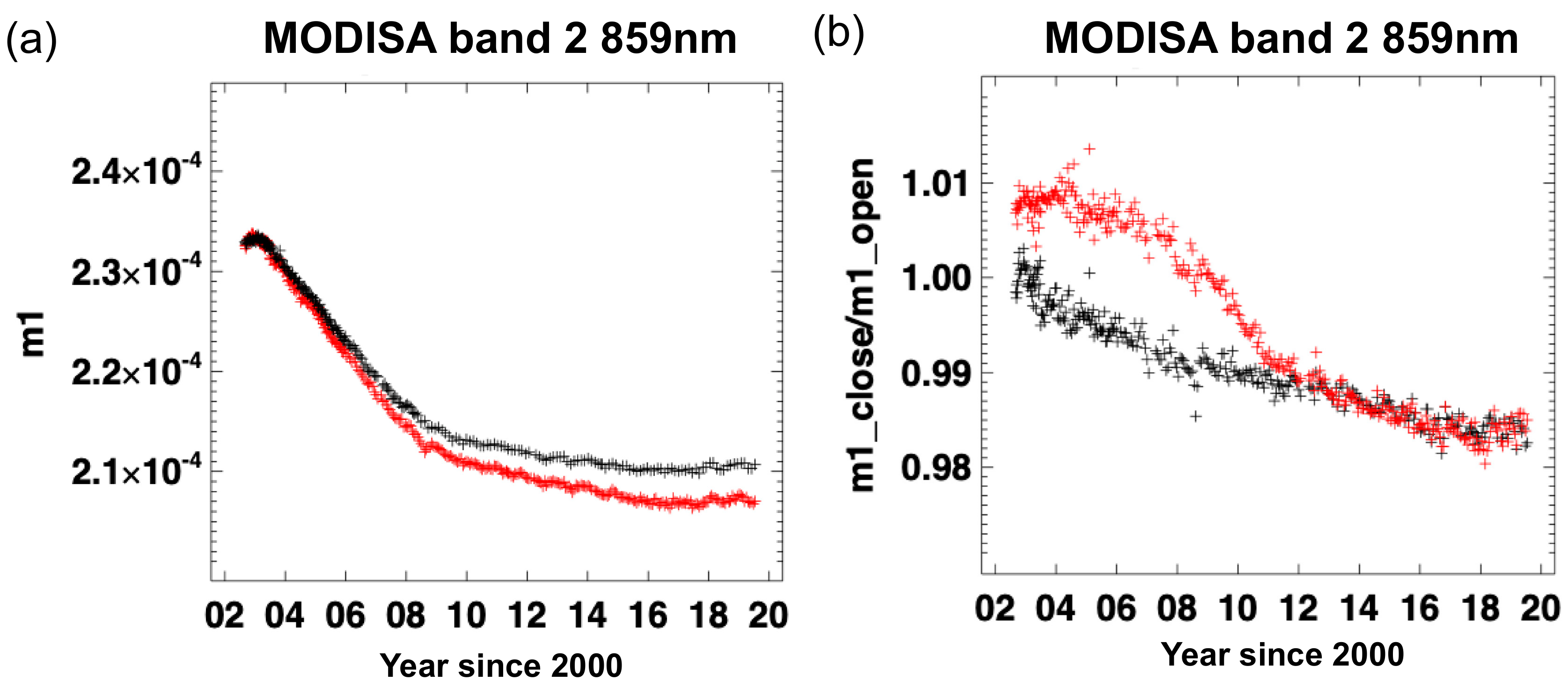
For MODIS land bands, the m1 can be computed by either SD screen open or closed data, as both high and low SD radiances are within the detectors’ dynamic range. Figure 7 shows that the band 2 detector gains computed using high (screen open) and low (screen closed) SD radiances have up to 1.5% differences. The ratios of m1 computed from high/low SD radiances also changed over time and are detector dependent. Since m1 is computed as the linear fit, the differences in high/low radiance m1 indicate the detector gain is not linear over the dynamic range. The temporal trend in high/low radiance m1 ratios indicates the detector response nonlinearity is changing over time. Figure 7b shows that the temporal change in detector response nonlinearity is detector dependent. Similar detector response nonlinearity behaviors are observed for most land band detectors, and the temporal change of detector response nonlinearities are most prominent for bands 1 and 2. The detector nonlinearity behavior is likely caused by the readout electronics as the detector gain of MODIS high-resolution bands (bands 1–4) have been shown to be subframe and radiance dependent [15]. To optimize calibration for ocean color products, we used low SD radiance data to compute m1 to better match the typical ocean surface radiance.
4.1.2. m1 Time Series
MODISA performs solar calibrations every 3 weeks after the first few years of operation [16]. The computed m1 (Figure 6 and Figure 7) has noise of up to 0.5 %. As the change in detector gain is expected to be gradual, a boxcar smoothing function is used to compute the running average of m1. The smoothing interval is set at 3 months for green and blue bands and 1 year for red and Near-InfraRed (NIR) bands. The smoothing intervals are selected to maximize the temporal m1 smoothness while retaining its temporal trend. In Figure 8, MODISA band 8 shows sharp changes in detector gains between 2011 and 2012. The same features are shown in the other blue and green bands with reduced magnitudes. The shorter smoothing time interval for blue/green bands is used to retain the temporal features. For red/NIR bands, the m1 changes are gradual and do not have distinct features (Figure 8b), and the longer interval is used to generate smoother m1 time series.
4.2. RVS
The RVS is the ratio of the detector response at a particular scan angle to the reference scan angle. In MODIS, the RVS is normalized to the SD angle, where the nominal detector gain (m1) is determined. Because the MODIS scan mirror is not protected, the MODISA RVS has changed significantly over time due to nonuniform mirror degradation [17]. We track the temporal RVS change by trending the instrument responses over pseudo-invariant calibration targets, i.e., SD, moon, and desert, observed at different scan angles [17,18]. For MODISA, the SD and moon are always observed at fixed scan angles. The desert can be observed at 16 angles from the repeatable orbital tracks. The SD is observed about every 3 weeks during solar calibration events. The moon is observed monthly except for the summer months when the moon is too close to the horizon. The desert site can be observed daily at one of the 16-day repeat scan angles, if the scene is free of clouds.
By comparing the relative trend difference at different scan angles, we can estimate the temporal change in RVS. The temporal trends at each angle and calibration target are normalized to the first measurement, and the RVS at each scan angle is compared relatively. Therefore, this method determines the change in RVS relative to the first measurement, where the Aqua RVS can be approximated as prelaunch measured values.
One of the limiting factors of this method is that the target brightness needs to be within the dynamic range of the detectors. Among the calibration targets, desert sites are too bright for bands 10 to 16 and certain parts of the moon are also too bright for bands 13 to 16, but the saturated moon pixel radiance can be estimated by the band ratioing method [19]. Therefore, for bands 1–9, 17–19, and 26, desert, moon, and SD are used to track RVS and only moon and SD are used to track RVS for bands 10–16 (Table 2).
Ideally, all calibration targets should have the same brightness to reduce the detector response nonlinearity impact. However, the brightness of SD, moon, and desert are significantly different, which adds additional uncertainty to RVS estimates using a combination of calibration targets.
The time-dependent RVS is computed by fitting 2nd-order polynomials over the temporal relative response vs. scan angles from all available calibration targets (Table 2). As described earlier, 2nd-order polynomials are more stable as they are less affected by noise in lunar and desert trends. The residual higher-order RVS behaviors are removed by the OBPG crosscalibration. This process optimizes the overall RVS correction for ocean color products when used in conjunction with OBPG crosscalibration. However, the temporal RVS by itself might not be the best possible RVS characterization for other disciplines without additional product specific corrections.
Since the RVS is normalized at the SD angle, the lunar and desert trends are computed using the time-dependent m1 (see Section 4.1), so the moon and desert trends are essentially the RVS trends at their respective observation angles. Using the time-dependent detector m1 for lunar and desert trends remove the potential uncertainties from temporal change in mirror side and detector-to-detector gain ratios. Using time-dependent detector m1 is especially important for lunar trends, as the moon is not a uniform target and cannot be evenly sampled among detectors. Because the moon image is an ellipsoid, more lunar pixels are sampled by middle detectors than the edge detectors. If the temporal gain ratios between middle and edge detectors changes, this will cause biases in the lunar trend.
4.2.1. Desert Trend
We used the Libya 4 site to track temporal RVS change. Libya 4 is one of the widely used pseudo-invariant sites due to its long-term surface reflectance stability [20]. Despite being a stable target, the satellite observations showed significant bidirectional reflectance distribution function (BRDF) effects with respect to solar incident and instrument view angles. A previous study characterized such effects by simultaneously fitting the solar incident, instrument view angles, and RVS changes [17]. Although this method can reduce the BRDF effects in the observed data, the method is empirical and requires a good assumption of the basic shape of RVS trends.
Since satellite observations are made with different geometrics between the sun and the instrument, the changing atmospheric path radiance from different solar incident and instrument view angles can cause the BRDF effect to be seen in the desert observation. To remove atmospheric contributions, an atmospheric model, 6SV [21], is used to estimate Rayleigh scattering and gaseous absorption. Figure 9 shows the band 8 mirror side 1 RVS characterization process at a −42-degree scan angle. The instrument TOA reflectance (Figure 9a) shows a large annual cycle. Figure 9b shows that the 6SV model estimated atmospheric contribution based on the solar and instrument view geometry. Figure 9b shows that the annual cycle of atmospheric contribution matches well with the annual variations of the TOA reflectance (Figure 9a). Removing the atmospheric contribution from TOA reflectance (Figure 9c) significantly reduces the annual cycles in the desert trending. In Figure 9c, the solar incident power and atmospherically corrected desert trend has a residual noise of a few percent, a significant reduction from the observed data. The residual noise in the desert trend could come from variations in aerosol, polarization effects, and possibly small short-term BRDF changes in the Libya 4 site itself.
To further demonstrate the importance of atmospheric correction, we compared the desert site RVS before and after atmospheric correction in January 2003 when the RVS should have minimal deviation from the prelaunch measured values. In Figure 10a, the sensor-observed TOA reflectance showed a 60% variation in response at different scan angles. After correcting for the atmospheric contribution, the RVS variation (Figure 10b) is significantly reduced. Since, the prelaunch measured RVS for band 8 is only about 2%, a 60% variation in RVS is unlikely after only 6 months of on-orbit operation. The results indicate the atmospheric correction removed the bulk of the instrument observation BRDF artifacts to improve RVS characterization accuracy.
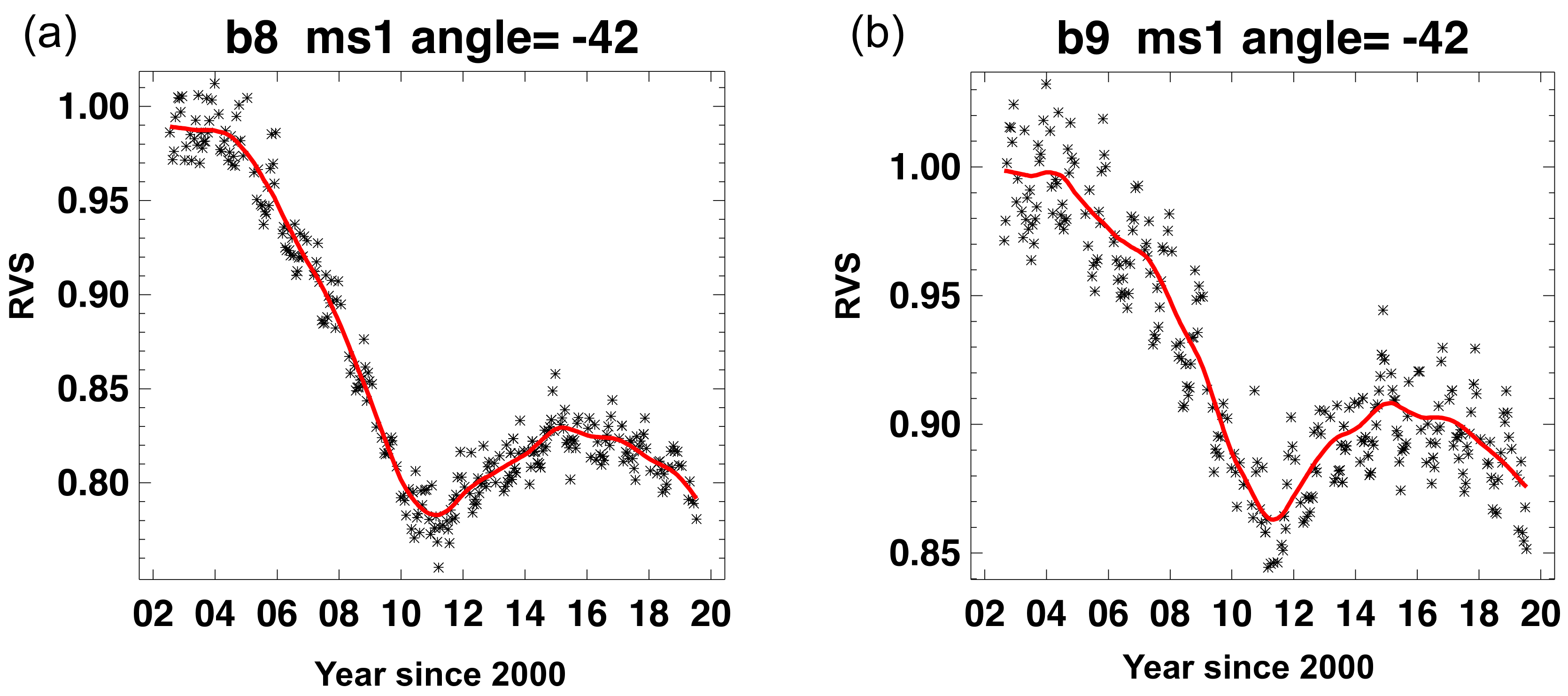
To reduce the residual noise in the atmospherically corrected desert trends, a 1-year running average was computed and used to produce smoothed temporal trends at each observation angle. Figure 11 shows examples of the computed desert trends and the smoothed RVS trends at −42 degrees for bands 8 and 9. The smoothed RVS desert trends will later be combined with lunar trends to characterize temporal RVS change.
4.2.2. Lunar Trend
The moon is an ideal calibration target, as its surface is photometrically stable [22] and it can be observed by MODIS without atmospheric contamination. The geometrically corrected lunar irradiance can be obtained from the US Geological Survey’s RObotic Lunar Observatory (ROLO) photometric model [23], using the observation time and the satellite position to determine the lunar phase and libration angles and sun–moon/satellite–moon distances. The lunar trend is computed as the ratio of the sensor-observed and model-predicted lunar irradiances. The temporal changes in the lunar trends provide the temporal RVS change at lunar observation angle [24].
The lunar trends (Figure 12) are normalized to the first observation to remove the residual biases between SD-calibrated and ROLO-predicted lunar irradiance. The normalized lunar trends are the temporal RVS changes at an Space View (SV) angle, which can be up to 20% in band 8 (412 nm). The temporal RVS changes are more prominent in the blue bands (8, 9, 3, and 10) and decrease at longer wavelengths. The temporal RVS trends resemble the m1 trends (Figure 8), where the trends in the blue bands reversed around 2011. For green to NIR bands, the temporal RVS changes are small with no clear reversing trends like the blue bands.
The lunar trends show a quasi-annual cycle, which is likely due to the residual uncertainty in the ROLO model’s libration correction [25]. To compute the RVS change at an SV angle, a 1-yr running average was computed to produce smoothed lunar trends, except for bands 8 and 9. A 2-piece fit was used for bands 8 and 9 before and after 2011 to better characterize the reversal in trends.
4.2.3. RVS Characterization
To characterize the temporal RVS, the available desert trends are combined with lunar trends. Since the lunar and desert trends are computed with time-dependent SD m1, the lunar/desert trends are the RVS normalized to SD angles. For bands 1–9, 17–19, and 26, the temporal RVS is estimated as a 2nd-order polynomial fit between the scan angle and the smoothed RVS from lunar and desert trends (Table 2). For bands 10–16, the RVS change is small (<4%) and only lunar trends were used to characterize the temporal RVS change. Since the moon is always observed at the same scan angle, we used the prelaunch estimated RVS curve as the basic shape to characterize the 2nd-order RVS fit from the lunar observation angle alone. This method assumes that small changes in RVS do not significantly change the shape of the RVS.
Figure 13 shows the characterized RVS for selected ocean bands and years. As mentioned earlier, band 8 has the largest temporal RVS change. In 2011, the RVS variation was the largest with the mirror response at the beginning of the scan (−55 degrees) ~30% higher than at the end of the scan (55 degrees). For the green to NIR bands, the RVS and their changes are considerably smaller.
4.3. Relative Spectral Response (RSR) Modulation
The temporal radiometric calibration for Aqua MODIS can be computed from the time-dependent m1 and RVS estimated in Section 4.1 and Section 4.2. The calibration coefficients convert the instrument response to TOA reflectance or radiance. However, the Aqua detector RSR has been shown to change over time due to the spectrally dependent optical degradation [12]. The temporal RSR change will cause bias in observed ocean radiances. Applying time-dependent RSR in ocean color product retrieval is not feasible due to complexity and computational time limitations. The current solution is to apply an adjustment in calibration coefficients to correct the estimate of the calibration bias in ocean color products due to RSR modulation.
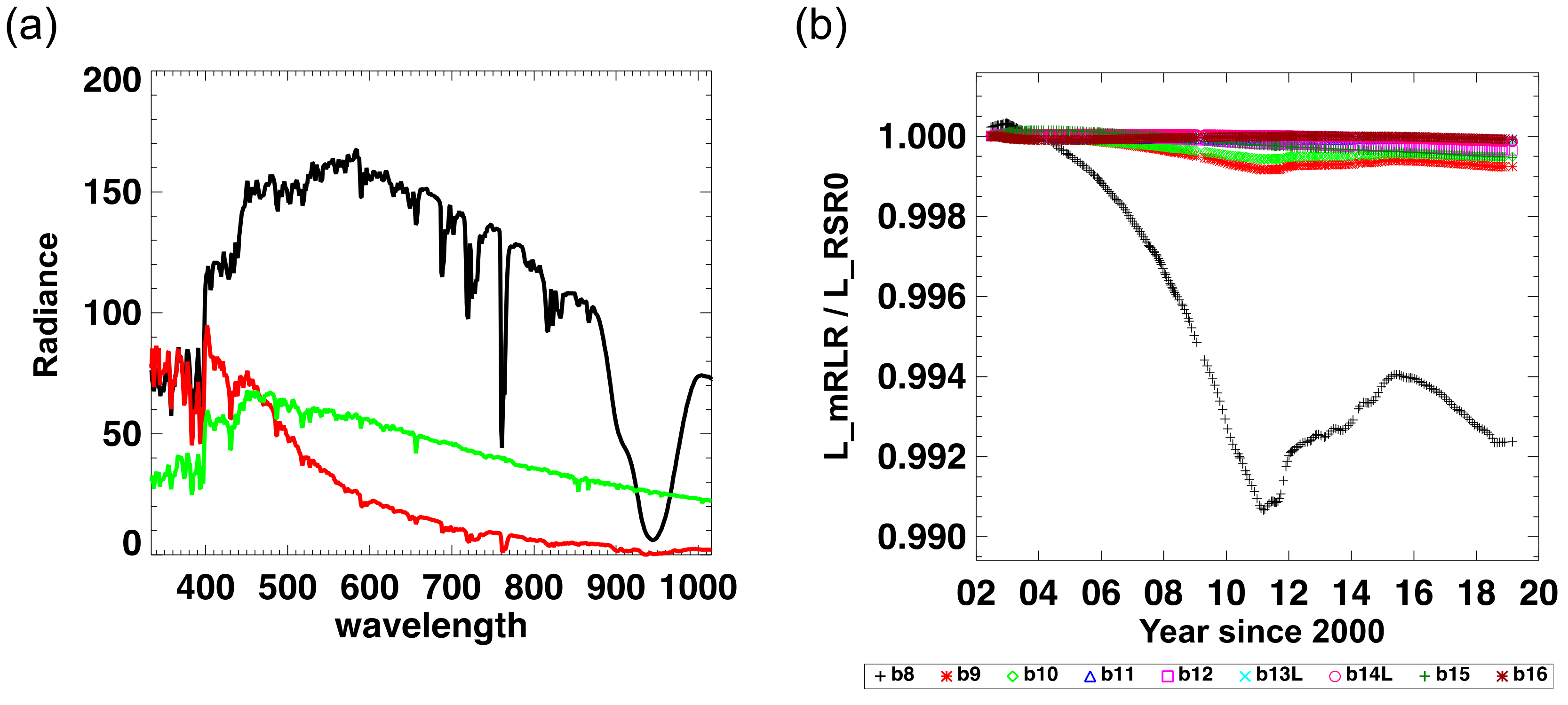
The derivation and correction of the time-dependent modulated RSR impact on Aqua ocean color products is detailed in our previous study [12]. The calibration bias due to RSR modulation is caused by the spectral differences between calibration targets and ocean scenes (Figure 14a). The RSR modulation impact on ocean color products is the combined effects of biases in observed SD, desert, and ocean scene radiances due to RSR modulation. Figure 14b shows the biases in ocean color product radiances due to modulated RSR computed using the typical spectral radiances in Figure 14a. Figure 14b shows that band 8 is the only band significantly impacted by RSR modulation with up to 1% biases in 2011. The large band 8 RSR modulation is the result of its large out-of-band response convolved with the large spectral radiance difference between calibration targets and the typical ocean scene. For the remaining ocean bands, the impacts from modulated RSR are less than 0.1%.
The biases of modulated RSR are estimated per band for all ocean bands (bands 8 to 16), where RSRs are measured for both in-band and out-of-band regions. Although the modulated RSR impact is dependent on scan angle due to the angular-dependent optical degradation [12], we apply the scan-angle mean impact for simplicity. The correction is meant to correct the bias in global radiometric trends. The angular dependency of modulated RSR impact is small and will be added to residual RVS characterization uncertainty and corrected by OBPG crosscalibration.
5. Results
5.1. OBPG RSB Calibration LUT
The main differences between OBPG and MCST calibration are summarized in Table 3. Additional differences could come from computation methodology and data selection. Figure 15 compares the temporal trends of band 8 m1 and RVS between OBPG and MCST LUT at selected scan angles. Figure 15 shows that the OBPG and MCST gain (m1/RVS) at an SD angle is within 1.5% different but can be up to 4% different at large scan angles. The RVS differences at an SD angle are the modulated RSR effects as described in Section 4.3. The scan-angle-dependent gain differences between OBPG and MCST LUT will change the global trends in ocean color products.
The OBPG RSB calibration LUTs are based on the MCST LUT with the time-dependent m1 and RVS coefficients replaced by the values derived in Section 4.1 and Section 4.2. The correction of modulated RSR impact is applied to RVS to keep the m1 coefficients as a pure product of solar calibration for better calibration traceability. Applying the modulated RSR correction to either m1 or RVS produces the same results.
Since the OBPG LUT retains the MCST LUT format, it can be used in MODIS L1B processing outside of OBPG. The OBPG produces a monthly updated LUT, based on the monthly updated MCST LUT to extend m1, RVS, and modulated RSR correction. The crosscalibration LUT (see following section) is also updated monthly after each new RSB LUT is generated to keep the correction up-to-date.
5.2. Artifact Mitigation
Based on the OBPG radiometric calibration LUT, vicarious and crosscalibrations were performed to correct absolute instrument calibration biases and to flat-field the residual RVS, mirror side, and detector-to-detector uncertainties [4,5]. The vicarious and crosscalibration were performed using Rrs products; therefore, any residual atmospheric correction errors will also be included. Without vicarious and crosscalibration, a perfectly calibrated sensor could still produce biased and/or stripped Rrs images due to residual error from atmospheric correction.
The vicarious calibration produces a constant factor for each band, which has no impact on temporal trends [5]. However, the residual RVS correction can potentially impact global temporal trends if the correction is large [4]. Figure 16 compares the crosscalibration-computed residual RVS correction (M11) between R2014 and R2018 products. The magnitude of R2018 M11 correction is smaller than the R2014 correction after 2011 and similar to before 2011. The R2014 M11 correction varies significantly after 2011, indicating RVS calibration issues. The large M11 correction will change the global temporal trends, as the mean earth scene correction is not 1. This is the case in R2014 products as the scene-averaged M11 correction changes significantly after 2011 (Figure 17).
In R2018 products, the M11 is normalized to ensure no temporal trends are introduced by the crosscalibration. Compared to R2014, the R2018 M11 has larger detector spread. This is because the MCST calibration incorporates detector-to-detector gain correction using ocean sites [11] for the calculation of their m1, whereas in R2018, the striping correction is applied only during the crosscalibration. There is no impact of the M11 detector spread on image quality in R2014 vs. R2018 after applying the OBPG crosscalibration.
6. Discussion
To demonstrate the impact of the calibration approach described in this paper, the ocean color products from the R2018 reprocessing are compared with the previous R2014 reprocessing. The only changes between these two reprocessing events were the updated instrument calibration approach and the updated vicarious calibration [26]. Figure 18 shows a comparison of the two reprocessing versions for the time series of spectral water-leaving reflectances (Rrs) and derived chlorophyll concentration, as derived from monthly averages for the globally distributed deepest ocean waters (>1000-m depth). We restrict our analysis to this deep-water subset as it allows for an assessment over the vast majority of the ocean surface while avoiding complex coastal regions with highly variable terrestrial influences. In Figure 18a, the R2014 water-leaving reflectances (solid lines) for the shortest wavelengths (412 nm and 443 nm) show a strong downward trend after 2012, which is not associated with any known geophysical events. This late-mission drift in the blue was significantly reduced in the R2018 products. Similarly, the large seasonal variability in the R2014 chlorophyll product, especially after 2012, is much reduced in the R2018 products (Figure 18b). Such variability will arise if the calibration in the blue is erroneously low, as the observed radiance has a strong seasonal cycle due to variations in solar geometry and associated atmospheric path radiance, and the correction for that variable atmospheric contribution to the TOA radiance will result in an underestimation of water-leaving reflectance in the blue. The chlorophyll concentration is derived from the ratio of blue to green water-leaving reflectances, such that a lower blue–green ratio implies a higher chlorophyll concentration, thus giving rise to seasonal peaks in the R2014 chlorophyll products. There is also an overall bias (increase) in the blue wavelengths between the R2014 and R2018 results, which is caused by an update to the vicarious calibration [26] and which also contributes to reduced seasonal variability in the R2018 chlorophyll product over the full mission lifetime.
Another very useful subset of the oceans for assessment of product temporal stability is the mean over the clearest ocean gyres, far from terrestrial influences, where chlorophyll concentrations are very low (typically <0.1 mg m-3) and homogenous, and weak variations in phytoplankton abundance or physiology, which modulate the absorption of blue light much more than green light, are the only significant influences on the ocean water optical properties. Temporal anomalies of water-leaving reflectance for the green ocean channel (547 nm) and green land channel (555 nm) were computed by subtracting the mean seasonal cycle from the water-leaving reflectance time series as derived over oligotrophic waters. In the absence of any major geophysical events, we can expect this time series to be relatively stable over time. The temporal anomalies for R2014 (Figure 19a,c) show a long-term trend and shorter-term variabilities that are larger than in the R2018 results (Figure 19b,d). Also notable is that the R2014 results for the two green bands with very similar center wavelengths (Figure 19a,c) are less consistent than the R2018 products (Figure 19 b,d). These results indicate that the R2018 products are more stable and consistent relative to the R2014 products.
7. Conclusions
In this paper, we described the independently developed MODIS Aqua radiometric calibration used in OBPG R2018 ocean color products. The OBPG calibration is developed based on the general MODIS calibration principles with a focus on ocean color products. The in-house developed calibration process is integrated in the ocean-color-product production cycle which enables fast evaluation. Timely product evaluation facilitates accurate assessment of the combined changes in radiometric calibration and the subsequent OBPG vicarious and crosscalibration. The integrated calibration development process is key to achieving the high radiometric calibration accuracy required for ocean color science.
Because the calibration is developed specifically for OBPG ocean color products, it is optimized for OBPG ocean color processing. For example, the nominal detector gains are calibrated with low SD radiance to better approximate ocean surface radiance. Applying the OBPG calibration for high-radiance targets could result in biases due to detector response nonlinearity. Furthermore, the RVS is characterized by simple 2nd-order fits to improve temporal stability. Applying the OBPG crosscalibration is needed to obtain the optimal RVS characterization.
Using the OBPG-developed radiometric calibration, the R2018 ocean color products show improved quality over the previous products (R2014). The global trends of the R2018 products are more stable and do not have late-mission anomalous behaviors shown in the R2014 products. The R2018 products are more consistent across wavelengths than R2014 products. Compared to the R2014 coefficients, the OBPG crosscalibration in R2018 is more consistent over time, indicating a more stable RVS characterization in R2018. The improvement in R2018 ocean-color-product quality and crosscalibration stability are the results of improvements in R2018 radiometric calibration.
Author Contributions
S.L. development the methodology, performed the analysis and wrote the manuscript. G.M. provided the advice, oversaw the progress and contributed to the writing and revising of the manuscript. B.F. contributed to the ocean color product validation processes and the writing and editing of the manuscript.
Funding
This research was funded by “Advancing the Quality and Continuity of Marine Remote Sensing Reflectance and Derived Ocean Color Products from MODIS to VIIRS” (17-TASNPP17-0065), submitted to the Science Mission Directorate’s Earth Science Division, in response to NASA Research Announcement (NRA) NNH17ZDA001N-TASNPP: Research Opportunities in Space and Earth Science (ROSES-2017).
Acknowledgments
The authors would like to thank MCST for providing in-depth knowledge of MODIS instrument characteristics and past and current calibration issues and developments.
Conflicts of Interest
The authors declare no conflict of interest.
Glossary
| Acronyms | Definition |
| 6SV | Atmospheric correction model. https://6s.ltdri.org/ |
| BOS | Beginning of the Scan |
| BRDF | Bidirectional Reflectance Distribution Function |
| BRF | Bidirectional Reflectance Function |
| Ecal | Electronic self Calibration |
| EOS | End of the Scan |
| H factor | Relative SD reflectivity |
| L1A | Formatted raw instrument data |
| L1B | Calibrated radiance computed from L1A |
| L2 | Derived per-pixel ocean color products L1B |
| L3 | Global binned ocean color products from L2 |
| LUT | Look-Up-Table |
| M1 | Detector radiometric gain coefficient |
| M1t | Time stamp of m1 |
| M11 | OBPG cross-calibration RVS correction coefficient |
| MCST | MODIS Calibration Support Team |
| MODIS | Moderate Resolution Imaging Spectroradiometer |
| MODISA | MODIS Aqua |
| MODIST | MODIS Terra |
| mRSR | Moduated RSR |
| NIR | Near-InfraRed |
| OBPG | Ocean Biological Processing Group |
| R2014 | https://oceancolor.qsfc.nasa.gov/reprocessing/r2014/aqua/ |
| R2018 | https://oceancolor.qsfc.nasa.gov/reprocessing/r2018/aqua/ |
| ROLO | RObotic Lunar Observatory |
| RSB | Reflective Solar Bands |
| RSR | Reflective Spectral Response |
| Rrs | Remote sensing reflectance |
| RVS | Response Versus Scan angle |
| RVSt | Time stamp of RVS |
| SAA | Solar Attanuation screen Assembly |
| SD | Solar Diffuser |
| SDSM | Solar Diffuser Stability Monitor |
| SIS | Spectral Integrating Sphere |
| SNR | Signal to Noise Ratio |
| SV | Space View |
| Tau | Screen transmission functions |
| TOA | Top of Atmosphere |
References
- Xiong, X.; Barnes, W.L.; Chiang, K.; Erives, H.; Che, N.; Sun, J.; Isaacman, A.T.; Salomonson, V.V. Status of Aqua MODIS on-orbit calibration and characterization. In Proceedings of the Sensors, Systems, and Next-Generation Satellites VIII, Maspalomas, Spain, 13–15 September 2004. [Google Scholar]
- Franz, B.A.; Kwiatowska, E.J.; Meister, G.; McClain, C.R. Moderate Resolution Imaging Spectroradiometer on Terra: Limitations for ocean color applications. J. Appl. Remote. Sens. 2008, 2, 23525. [Google Scholar] [CrossRef]
- Meister, G.; Eplee, R.E.; Franz, B.A. Corrections to MODIS Terra calibration and polarization trending derived from ocean color products. In Proceedings of the Earth Observing Systems XIX, San Diego, CA, USA, 18–20 August 2014. [Google Scholar]
- Meister, G.; Franz, B.A. Corrections to the MODIS Aqua Calibration Derived from MODIS Aqua Ocean Color Products. IEEE Trans. Geosci. Remote. Sens. 2014, 52, 6534–6541. [Google Scholar] [CrossRef]
- Franz, B.A.; Bailey, S.W.; Werdell, P.J.; McClain, C.R. Sensor-independent approach to the vicarious calibration of satellite ocean color radiometry. Appl. Opt. 2007, 46, 5068–5082. [Google Scholar] [CrossRef] [PubMed]
- Franz, B.A. Status of MODIS and VIIRS OC & SST Production & Distribution. In Proceedings of the MODIS/VIIRS Science Team Meeting, Silver Spring, MD, USA, 6–10 June 2016. [Google Scholar]
- Turpie, K.R.; Eplee, R.E.; Franz, B.A.; Del Castillo, C. Calibration uncertainty in ocean color satellite sensors and trends in long-term environmental records. SPIE Sens. Technol. Appl. 2014, 9111, 911103. [Google Scholar]
- Franz, B.A.; Bailey, S.W.; Meister, G.; Werdell, P.J. Consistency of the NASA Ocean Color Data Record. In Proceedings of the Ocean Optics 2012, Glasgow, UK, 8–12 October 2012. [Google Scholar]
- International Ocean-Colour Coordinating Group. In-Flight Calibration of Satellite Ocean-Colour Sensors; Report Number 14; International Ocean Colour Coordinating Group: Dartmouth, NS, Canada, 2013. [Google Scholar]
- MODIS Characterization and Calibration Team. MODIS Instrument Operations Status. In Proceedings of the MODIS/VIIRS Science Team Meeting, Silver Spring, MD, USA, 15–19 October 2018. [Google Scholar]
- Sun, J.; Angal, A.; Chen, H.; Geng, X.; Wu, A.; Choi, T.; Chu, M. MODIS reflective solar bands calibration improvements in Collection 6. In Proceedings of the Earth Observing Missions and Sensors: Development, Implementation, and Characterization II, Bertinoro, Italy, 25–28 June 2012. [Google Scholar]
- Lee, S.; Meister, G. MODIS Aqua Optical Throughput Degradation Impact on Relative Spectral Response and Calibration of Ocean Color Products. IEEE Trans. Geosci. Remote Sens. 2017, 55, 5214–5219. [Google Scholar] [CrossRef]
- Xiong, X.; Sun, J.-Q.; Esposito, J.A.; Guenther, B.; Barnes, W.L. MODIS reflective solar bands calibration algorithm and on-orbit performance. In Proceedings of the Optical Remote Sensing of the Atmosphere and Clouds III, Québec City, QC, Canada, 3–6 February 2003. [Google Scholar]
- Lee, S.; Meister, G. MODIS solar diffuser degradation determination and its spectral dependency. In Proceedings of the Earth Observing Systems XXIII, San Diego, CA, USA, 21–23 August 2018. [Google Scholar]
- Meister, G.; Pan, C.; Patt, F.S.; Franz, B.; Xiong, J.; McClain, C.R. Correction of subframe striping in high-resolution MODIS ocean color products. In Proceedings of the Earth Observing Systems XII, San Diego, CA, USA, 10–14 August 2007. [Google Scholar]
- MODIS Characterization Support Team. Available online: https://mcst.gsfc.nasa.gov/ (accessed on 12 September 2019).
- Sun, J.; Xiong, X.; Angal, A.; Chen, H.; Wu, A.; Geng, X. Time-Dependent Response Versus Scan Anglefor MODIS Reflective Solar Bands. IEEE Trans. Geosci. Remote Sens. 2013, 52, 3159–3174. [Google Scholar] [CrossRef]
- Xiong, X.; Salomonson, V.V.; Chiang, K.-F.; Wu, A.; Guenther, B.W.; Barnes, W. On-orbit characterization of RVS for MODIS thermal emissive bands. In Proceedings of the Passive Optical Remote Sensing of the Atmosphere and Clouds IV, Honolulu, Hi, USA, 9–10 November 2004. [Google Scholar]
- Xiong, X.; Geng, X.; Angal, A.; Sun, J.; Barnes, W. Using the Moon to track MODIS reflective solar bands calibration stability. In Proceedings of the Sensors, Systems, and Next-Generation Satellites XV, Prague, Czech Republic, 19–22 September 2011. [Google Scholar]
- Helder, D.L.; Basnet, B.; Morstad, D.L. Optimized identification of worldwide radiometric pseudo-invariant calibration sites. Can. J. Remote. Sens. 2010, 36, 527–539. [Google Scholar] [CrossRef]
- Vermote, E.F.; Tanré, D.; Deuzé, J.L.; Herman, M.; Morcrette, J.-J. Second Simulation of the Satellite Signal in the Solar Spectrum, 6S: An Overview. IEEE Trans. Geosci. Remote Sens. 1997, 35, 675–686. [Google Scholar] [CrossRef]
- Kieffer, H.H. Photometric Stability of the Lunar Surface. Icarus 1997, 130, 323–327. [Google Scholar] [CrossRef]
- Kieffer, H.H.; Stone, T.C. The Spectral Irradiance of the Moon. Astron. J. 2005, 129, 2887–2901. [Google Scholar] [CrossRef] [Green Version]
- Sun, J.-Q.; Xiong, X.; Barnes, W.L.; Guenther, B. MODIS Reflective Solar Bands On-Orbit Lunar Calibration. IEEE Trans. Geosci. Remote. Sens. 2007, 45, 2383–2393. [Google Scholar] [CrossRef]
- Bailey, S.W. On-orbit calibration of the Suomi National Polar-Orbiting Partnership Visible Infrared Imaging Radiometer Suite for ocean color applications. Appl. Opt. 2015, 54, 1984. [Google Scholar] [CrossRef]
- Franz, B.A.; Bailey, S.W.; Eplee, R.E., Jr.; Lee, S.; Patt, F.S.; Proctor, C.; Meister, G. NASA Multi-Mission Ocean Color Reprocessing 2018. In Proceedings of the Ocean Optics XXIV, Dubrovnik, Croatia, 8–12 October 2018; Available online: https://www.researchgate.net/publication/331652881_NASA_Multi-Mission_Ocean_Color_Reprocessing_20180 (accessed on 12 September 2019).
Figure 1.
Ocean Biological Processing Group (OBPG) ocean color production process: L1A is the formatted raw instrument data. L1B is the calibrated radiance. L2/L3 are the level 2 and 3 ocean color products [8].
Figure 1.
Ocean Biological Processing Group (OBPG) ocean color production process: L1A is the formatted raw instrument data. L1B is the calibrated radiance. L2/L3 are the level 2 and 3 ocean color products [8].

Figure 2.
Aqua RSB calibration procedures: The calibration process produces an RSB look-up-table (LUT), which contains temporal gain (m1) and response versus scan angle (RVS) parameters at time steps of m1t and RVSt respectively. The grey boxes are the source data; the yellow boxes are the calibration processes; the intermediate calibration parameters are outlined by red lines; and the red box is the final product of RSB calibration LUT. Ecal: electronic self-calibration; Yaw: spacecraft yaw maneuver.

Figure 3.
Schematic of solar diffuser (SD)/SDSM calibration assembly. The SD sunscreen has ~7.5% transmission and SDSM sunscreen has ~1.4% transmission.
Figure 3.
Schematic of solar diffuser (SD)/SDSM calibration assembly. The SD sunscreen has ~7.5% transmission and SDSM sunscreen has ~1.4% transmission.

Figure 4.
(a) SD reflectivity (H) for SDSM detectors 1 to 9 and (b) SD wavelength model-estimated SD degradation at MODIS Aqua (MODISA) bands 5 (1240 nm), 6 (1640 nm), and 7 (2130 nm).
Figure 4.
(a) SD reflectivity (H) for SDSM detectors 1 to 9 and (b) SD wavelength model-estimated SD degradation at MODIS Aqua (MODISA) bands 5 (1240 nm), 6 (1640 nm), and 7 (2130 nm).

Figure 5.
Comparison of typical ocean radiance (blue curve) and average Aqua SD radiance with (SAA_close) and without (SAA_open) SD attenuation screen assembly.
Figure 5.
Comparison of typical ocean radiance (blue curve) and average Aqua SD radiance with (SAA_close) and without (SAA_open) SD attenuation screen assembly.

Figure 6.
MODISA band 9 SD calibration: (a) detector 1 background-subtracted, temperature-corrected dn at SD view for screen open (black) and screen closed (red) and (b) computed m1 for detector 1 (black) and detector 10 (red).
Figure 6.
MODISA band 9 SD calibration: (a) detector 1 background-subtracted, temperature-corrected dn at SD view for screen open (black) and screen closed (red) and (b) computed m1 for detector 1 (black) and detector 10 (red).

Figure 7.
MODISA band 2 SD calibration: (a) detector 1 m1 computed from screen open (black) and closed (red) data and (b) ratios of m1 computed using SD screen open and closed data for detectors 1 (black) and 10 (red).
Figure 7.
MODISA band 2 SD calibration: (a) detector 1 m1 computed from screen open (black) and closed (red) data and (b) ratios of m1 computed using SD screen open and closed data for detectors 1 (black) and 10 (red).

Figure 8.
MODISA-normalized m1 computed from SD calibrations (symbols) and the smoothed m1 used for calibration (red curve) for mirror side 1 and detector 1 of (a) band 8 and (b) band 16.
Figure 8.
MODISA-normalized m1 computed from SD calibrations (symbols) and the smoothed m1 used for calibration (red curve) for mirror side 1 and detector 1 of (a) band 8 and (b) band 16.

Figure 9.
Desert trend for Aqua band 8, mirror side 1 at a scan angle of −42 degrees: (a) top-of-atmosphere (TOA) reflectance; (b) atmospheric contribution in reflectance; and (c) TOA reflectance—atmospheric reflectance. The TOA reflectance is computed using Equation (1) with RVS set to 1.
Figure 9.
Desert trend for Aqua band 8, mirror side 1 at a scan angle of −42 degrees: (a) top-of-atmosphere (TOA) reflectance; (b) atmospheric contribution in reflectance; and (c) TOA reflectance—atmospheric reflectance. The TOA reflectance is computed using Equation (1) with RVS set to 1.

Figure 10.
Libya 4 desert observations for MODISA band 8, mirror side 1 during 2003 January: The plots show the normalized reflectance (ref) versus scan angle (RVS) before (a) and after (b) atmospheric correction. Notice in some angles, 2 clear sky observations were made from the 16-day repeat orbits in January 2003.

Figure 11.
RVS computed from desert trends of MODISA mirror side 1 for (a) band 8 and (b) band 9 at a −42-degree scan angle: The black symbols are the computed RVS at each desert observation, and the red curve is the temporal smoothed RVS.
Figure 11.
RVS computed from desert trends of MODISA mirror side 1 for (a) band 8 and (b) band 9 at a −42-degree scan angle: The black symbols are the computed RVS at each desert observation, and the red curve is the temporal smoothed RVS.

Figure 12.
MODISA lunar trends for selected RSBs for (a) mirror side 1 and (b) mirror side 2: The symbols indicate each lunar calibration data point, and the curves are the fitted lunar trends.
Figure 12.
MODISA lunar trends for selected RSBs for (a) mirror side 1 and (b) mirror side 2: The symbols indicate each lunar calibration data point, and the curves are the fitted lunar trends.

Figure 13.
MODISA RVS fitting at selected years for (a) band 8 (412 nm), (b) band 12 (547 nm), and (c) band 16 (869 nm), mirror side 1.
Figure 13.
MODISA RVS fitting at selected years for (a) band 8 (412 nm), (b) band 12 (547 nm), and (c) band 16 (869 nm), mirror side 1.

Figure 14.
(a) Typical radiance for ocean (red), SD (green), and the desert (black) and (b) mean calibration bias (L_mRSR/L_RSR0) due to modulated RSR for bands 8 to 16: L_mRSR is the typical ocean radiance computed using modulated RSR (mRSR), and L_RSR0 is the typical ocean radiance computed using prelaunch measured RSR (RSR0).

Figure 15.
Time series of OBPG and MCST mirror side 1, detector-averaged normalized band 8 for (a) m1 and (b) RVS and (c,d) their differences at SD, space view (SV), Nadir, beginning of scan (BOS; −55 degrees), and end of scan (EOS; 55 degrees). Solid line: OBPG, dashed line: MCST. Colors indicate scan angles. The scan angle-specific detector gain is computed as m1/RVS, and m1_t0 is the SD m1 at the beginning of the mission. Note: the legend in Figure 15a is applied to Figure 15b–d.

Figure 16.
Band 8 (412 nm), mirror side 1, detector 1, crosscalibration correction factors (M11) for select years: (a) R2018 calibration and (b) R2014 calibration. M11 is the RVS correction (unitless).
Figure 16.
Band 8 (412 nm), mirror side 1, detector 1, crosscalibration correction factors (M11) for select years: (a) R2018 calibration and (b) R2014 calibration. M11 is the RVS correction (unitless).

Figure 17.
Time series of band 8, mirror side 1, scan-averaged M11 correction for (a) R2018 and (b) R2014 products: The scan-angle-averaged M11_avg indicates the correction on the global mean. Colors indicate detectors 1–10.
Figure 17.
Time series of band 8, mirror side 1, scan-averaged M11 correction for (a) R2018 and (b) R2014 products: The scan-angle-averaged M11_avg indicates the correction on the global mean. Colors indicate detectors 1–10.

Figure 18.
MODIS global deep-water temporal trends for (a) water-leaving reflectance (Rrs) and (b) chlorophyll. Solid line: R2018, dashed line: R2014 products.
Figure 18.
MODIS global deep-water temporal trends for (a) water-leaving reflectance (Rrs) and (b) chlorophyll. Solid line: R2018, dashed line: R2014 products.

Figure 19.
MODIS water-leaving reflectance (Rrs) temporal anomaly in global oligotrophic water: (a,c) R2014 products for 547 nm and 555 nm and (b,d) R2018 products for 547 nm and 555 nm.
Figure 19.
MODIS water-leaving reflectance (Rrs) temporal anomaly in global oligotrophic water: (a,c) R2014 products for 547 nm and 555 nm and (b,d) R2018 products for 547 nm and 555 nm.


Table 1.
Moderate Resolution Imaging Spectroradiometer (MODIS) solar diffuser stability monitor (SDSM) detectors and reflective solar bands (RSB) center wavelengths.
Table 1.
Moderate Resolution Imaging Spectroradiometer (MODIS) solar diffuser stability monitor (SDSM) detectors and reflective solar bands (RSB) center wavelengths.
| SDSM | Wavelength | Land/Atmosphere | Center Wavalength (nm) | Band Width (nm) | Ocean | Center Wanalength | Band Width (nm) |
|---|---|---|---|---|---|---|---|
| Detector 1 | 412 | Band 1 | 645 | 50 | Band 8 | 412 | 15 |
| Detector 2 | 466 | Band 2 | 859 | 35 | Band 9 | 443 | 10 |
| Detector 3 | 530 | Band 3 | 469 | 20 | Band 10 | 488 | 10 |
| Detector 4 | 554 | Band 4 | 555 | 20 | Band 11 | 531 | 10 |
| Detector 5 | 646 | Band 5 | 1240 | 20 | Band 12 | 551 | 10 |
| Detector 6 | 747 | Band 6 | 1640 | 24 | Band 13 | 667 | 10 |
| Detector 7 | 857 | Band 7 | 2130 | 50 | Band 14 | 678 | 10 |
| Detector 8 | 904 | Band 17 | 905 | 30 | Band 15 | 748 | 10 |
| Detector 9 | 936 | Band 18 | 936 | 10 | Band 16 | 869 | 10 |
| Band 19 | 940 | 50 | |||||
| Band 26 | 1375 | 30 |
Table 2.
Calibration targets used to track MODISA temporal RVS change and fitting function used for RVS characterization. The desert site is not used for bands 10–16 due to saturation.
Table 2.
Calibration targets used to track MODISA temporal RVS change and fitting function used for RVS characterization. The desert site is not used for bands 10–16 due to saturation.
| Bands | Calibration Targets | RVS Characterization |
|---|---|---|
| Bands 1–9 Bands 17–19 Bans 26 | Moon, SD, desert | 2nd order polynomial |
| Bands 10–16 | Moon, SD | 2nd order polynomial |
Table 3.
Calibration methodology differences between R2014 and R2018.
| R2014 * | R2018 | |
|---|---|---|
| SDSM calibration | Detector 9 normalization Sd/SDSM screen for detector 9 degradation | Detector 9 normalization refined by SD/SDSM screen SDSM wavelength model for interpolation and detector 9 degradation |
| SD calibration | Use highest SD unsaturated signal to maximize SNR | Use low SD signal for all bands to better match ocean radiance |
| Temporal RVS characterization | 2nd to 4th order fit Remove BRDF effect by fitting observed data vs. view and illumination geometric | 2nd order fit for all bands Use atmospheric correction to remove BRDF effect Apply modulated RSR impact |
© 2019 by the authors. Licensee MDPI, Basel, Switzerland. This article is an open access article distributed under the terms and conditions of the Creative Commons Attribution (CC BY) license (http://creativecommons.org/licenses/by/4.0/).
Share and Cite
MDPI and ACS Style
Lee, S.; Meister, G.; Franz, B. MODIS Aqua Reflective Solar Band Calibration for NASA’s R2018 Ocean Color Products. Remote Sens. 2019, 11, 2187. https://doi.org/10.3390/rs11192187
AMA Style
Lee S, Meister G, Franz B. MODIS Aqua Reflective Solar Band Calibration for NASA’s R2018 Ocean Color Products. Remote Sensing. 2019; 11(19):2187. https://doi.org/10.3390/rs11192187
Chicago/Turabian StyleLee, Shihyan, Gerhard Meister, and Bryan Franz. 2019. "MODIS Aqua Reflective Solar Band Calibration for NASA’s R2018 Ocean Color Products" Remote Sensing 11, no. 19: 2187. https://doi.org/10.3390/rs11192187
Note that from the first issue of 2016, this journal uses article numbers instead of page numbers. See further details here.