Deep Cube-Pair Network for Hyperspectral Imagery Classification

Abstract

Advanced classification methods, which can fully utilize the 3D characteristic of hyperspectral image (HSI) and generalize well to the test data given only limited labeled training samples (i.e., small training dataset), have long been the research objective for HSI classification problem. Witnessing the success of deep-learning-based methods, a cube-pair-based convolutional neural networks (CNN) classification architecture is proposed to cope this objective in this study, where cube-pair is used to address the small training dataset problem as well as preserve the 3D local structure of HSI data. Within this architecture, a 3D fully convolutional network is further modeled, which has less parameters compared with traditional CNN. Provided the same amount of training samples, the modeled network can go deeper than traditional CNN and thus has superior generalization ability. Experimental results on several HSI datasets demonstrate that the proposed method has superior classification results compared with other state-of-the-art competing methods.

1. Introduction

A hyperspectral image (HSI) is a 3D (three dimensional) datacube containing both spectral and spatial information [1,2,3,4,5,6,7]. Compared with the traditional image (e.g., RGB image), an HSI contains a continuous spectrum at each pixel, which facilitates many remote-sensing-related applications [8,9,10,11,12,13,14,15,16,17], such as resource exploration, environment monitoring, land-use mapping, and water pollution detection.

HSI classification has been one of the most popular research areas for HSI analysis in the past several decades, which aims at assigning each pixel a pre-defined class label. Numerous methods thus have been proposed for HSI classification, which can be roughly divided into non-deep-earning-based and deep-learning-based methods [18,19,20,21,22,23,24,25,26]. Classifiers and feature extractions are two ingredients of non-deep-learning-based HSI classification methods [27], among which typical classifiers include k-nearest neighbor (k-NN) [28,29], logistic regression (LR) [30,31,32], and support vector machine (SVM) [33,34,35,36]. By evaluating the distances between the training samples/pixels and the test sample, the k-NN method selects k training samples that have the smallest distance to the test sample and then assigns the test sample a label which dominates the selected k training samples. The logistic regression method is proposed for HSI classification considering it has the merit to estimate class probabilities directly using the logit transform. The SVM seeks to trace an optimal hyperplane that linearly separates features into two groups with a maximum margin, which shows a powerful capability of classifying hyperspectral data. In addition, for non-deep-learning-based HSI classification methods, feature extraction methods, such as principal component analysis (PCA) [37], independent component analysis (ICA) [38], and minimum noise fraction (MNF) [39], are always used together with the above classifiers to cope with the high-dimensionality and nonlinearity of the data. However, two problems limit the performance of non-deep-learning-based HSI classification methods. (1) They use shallow structures (i.e., the SVM can be attributed to a single-layer classifier, while PCA can be seen as a single-layer feature extractor), which have limited nonlinear representation capability and may not be able to represent the nonlinearity in the HSI. (2) The features adopted are usually hand-crafted, which may not fit the classification task very well.

In contrast, deep learning methods [40,41,42,43,44,45,46,47,48,49] are based on multi-layer structures and thus have superior nonlinear representation ability. The stack autoencode (SAE) [44,48,50,51] and the convolutional neural network (CNN) [40,41,42,45,52] are two representative categories. A commonly used strategy in building an SAE model includes unsupervised pretraining over the unlabeled samples first and then a supervised fine-tuning over the labeled samples. The deep belief network (DBN) [53,54] also belongs to this category, where unsupervised pretraining over the unlabeled samples is accomplished via the DBN instead of the SAE. Compared with the SAE, the CNN is a completely supervised deep learning method and shows a more powerful classification capability since it intergrates feature extraction and a classifier naturally into one framework (i.e., the extracted feature is specific to the classifier). Thus, we focus on CNN-based HSI classification method in this study. Some CNN-based methods have been proposed. Hu et al. [42] proposes a CNN-based method based on spectral information only. Slavkovikj et al. [46] incorporates both spatial and spectral information into CNN within a local patch structure. Zhang et al. [41] proposes a dual-stream CNN, where one stream extracts the spectral feature and the other stream extracts the spatial-spectral feature. Chen et al. [47] and Li et al. [45] propose a 3D CNN network to consider the 3D structure of HSI data.

Two characteristics are considered important for HSI classification. First, an HSI is inherently a 3D datacube, which contains both spectral and spatial structure. However, the majority of existing CNN-based HSI classification methods consider spectral only, or destroy the original correlation between spatial and spectral without fully considering the useful 3D structure. Second, since labeling an HSI is tedious, expensive, and can only be accomplished by experts, labeled pixels provided for HSI classification are limited. However, all CNN-based methods demand large amounts of labeled samples due to a huge amount of parameters in the network, and more parameters will be generated as CNN has a deeper structure. Given limited labeled samples, many CNN-based methods cannot be fully trained, i.e., the generalization ability of the neural network is unsatisfactory with insufficiently labeled data. To address these problems, inspired by the newly proposed pixel-pair feature [40], we propose a cube-pair-based CNN classification architecture in this study, where cube-pair is used to enhance the training sample and to model the local 3D structure simultaneously. Within this architecture, a 3D fully convolutional network (FCN) is further modeled, which has fewer parameters compared with the traditional CNN. Provided the same amount of training samples, the modeled network can go deeper than the traditional CNN and thus has superior generalization ability for HSI classification. The main ideas and contributions are summarized as follows.

(1)

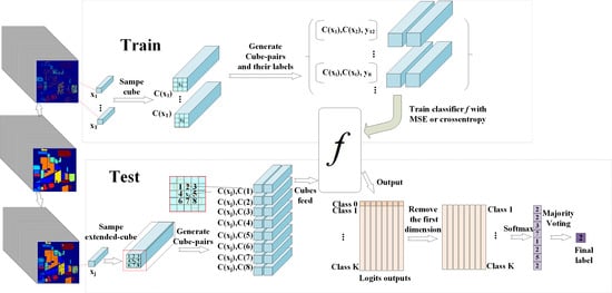
Cube-pair is used when modeling CNN classification architecture. The advantage of using cube-pair is that it can not only generate more samples for training but can also utilize the local 3D structure directly.

(2)

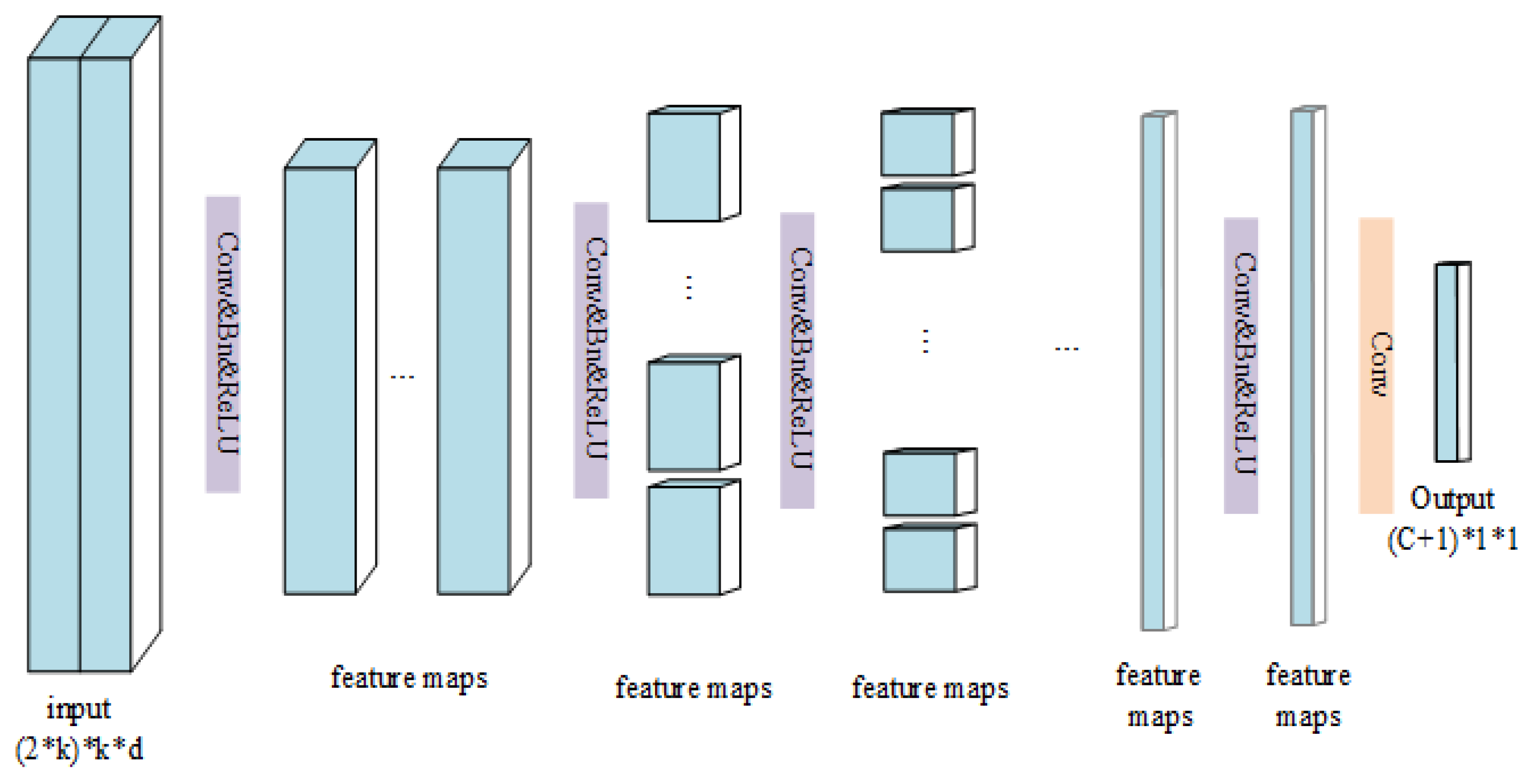
A 3D FCN is modeled within a cube-pair-based HSI classification architecture, which is a deep end-to-end 3D network pertinent for the 3D structure of HSI. In addition, it has fewer parameters than the traditional CNN. Provided the same amount of training samples, the modeled network can go deeper than traditional CNN and thus has superior generalization ability.

(3)

The proposed method obtains the best classification results, compared with the pixel-pair CNN and other deep-learning-based methods.

The remainder of this paper is structured as follows. Section 2 describes the deep cube-pair network for HSI classification including the cube-pair-based CNN classification architecture and the cube-pair-based FCN. Experimental results and analysis are provided in Section 3. Section 4 concludes the paper.

2. The Deep Cube-Pair Network for HSI Classification

First, we categorize the existing CNN-based methods into three categories in Section 2.1, which include pixel-based architecture, pixel-pair-based architecture, and cube-based architecture. We then propose a new cube-pair-based HSI classification architecture that takes advantage of both cube-based and pixel-pair-based methods in Section 2.2. Since any kind of 3D deep neural network can be used within this architecture (i.e., acting as a cube-pair network), we give a brief introduction of cube-pair-based HSI classification architecture including cube-pair generation for training and test procedures, and the class label inference for the test data. Finally, we model a specific 3D deep neural network in Section 2.3. We introduce the structure of the modeled 3D fully convolutional network in detail and briefly introduce its training and test strategies.

2.1. Mathematical Formulation of Commonly Used CNN-Based HSI Classification Architecture

In this study, we denote $X\in {\mathbb{R}}^{w\times h\times d}$ as an HSI dataset, where w, h, and d represent the width, height, and bands (i.e., spectral channels/wavelengths), respectively. Among the total number of $w\times h$ pixels, N pixels are labeled and denoted as training set $\mathbb{T}={\left\{x_i,y_i\right\}}_{i=1}^N$, where $x_i\in {\mathbb{R}}^d$ is a d-dimensional spectrum of one pixel, and $y_i$ is its corresponding label chosen from $\mathbb{K}=\left\{1,\cdots ,K\right\}$. K is the total number of classes.

Pixel-level-based HSI classification architecture is a commonly used architecture, which is on the pixel level. Specifically, a prediction function as follows is learned.

$$\begin{array}{c}\hfill f:x_i\mapsto y_i,\mathrm{where}i\in \left\{1,\cdots ,N\right\}.\end{array}$$

(1)

Then, the learned function f is used to assign labels for unlabeled pixels $x_j\notin \mathbb{T}$. In this study, f represents CNN-based methods.

A pixel-pair-based architecture is proposed to address the small training dataset problem. For an HSI, only limited labeled samples can be provided in real conditions (i.e., N is small) since labeling HSI is tedious and expensive, and can only be accomplished by experts. However, the CNN (i.e., f) always demands large amounts of labeled training samples (i.e., where N is large) to train the parameters, especially when the network goes deeper. To address this contradiction, Li et al. [40] proposed a pixel-pair-based HSI classification architecture, where they reformulated pixel-level classification architecture as

$$\begin{array}{c}\hfill f:(x_i,x_t)\mapsto y_{it},\mathrm{where}i,t\in \left\{1,\cdots ,N\right\}.\end{array}$$

(2)

The label $y_{it}$ for the pixel-pair $\left\{x_i,x_t\right\}$ in [40] is determined by

$$\begin{array}{c}\hfill y_{it}=\left\{\begin{array}{ccc}\hfill l& if\hfill & y_i=y_t=l,\hfill \\ \hfill 0& if\hfill & y_i\ne y_t.\hfill \end{array}\right.\end{array}$$

(3)

Though the number of labeled pixels may be limited, it can be seen that the number of labeled pixel-pairs can be huge since the combination of pixels in the training set is larger than the number of training pixels (square-level magnitude for pixel-pair versus the original number for pixel), which mitigates the gap between the number HSI can be provided for training and the number deep learning methods demanded. Then, a pixel-pair network (e.g., f) is constructed based on pixel-pairs. Finally, a voting strategy is proposed to obtain the final classification result for the test pixel based on the value output from f. Though it can effectively increase the training sample, the useful 3D structure is ignored for a pixel-pair-based architecture.

Cube-based architecture is proposed to directly use 3D structure of HSI for classification, which can be represented as

$$\begin{array}{c}\hfill f:C\left(x_i\right)\mapsto y_i,\mathrm{where}i\in \left\{1,\cdots ,N\right\}.\end{array}$$

(4)

$C{\left(x_i\right)}^k\in {\mathbb{R}}^{k\times k\times d}$ represents a local cube centered at $x_i$, whose width k equals the height. The basic idea using Equation (4) is that spatial neighboring pixels tend to have the same class label. However, a cube-based architecture alone does not address the small training dataset problem, i.e., f in Equation (4) still needs a large amount of training samples. In addition, though a cube-based architecture is proposed to model 3D structure of HSI, the majority of existing CNN-based HSI classification methods do not model 3D data directly. Those methods reshape the original 3D tensor structure of HSI into vectors and matrices first, then construct a 1D or 2D CNN network based on the reshaped data. Though those methods capture spectral and spatial information to some extent, the original 3D structure (e.g., the correlation between spatial and spectral) is destroyed accomplished with reshaping, which influences the performance of HSI classification results.

2.2. The Cube-Pair-Based CNN Classification Architecture

2.2.1. The Proposed Architecture

A small sample and a 3D structure are two important characteristics of an HSI. However, as shown above, pixel-pair-based and cube-based architecture address only one. To the best of our knowledge, no existing architecture utilizes them simultaneously, which inspires us to propose cube-pair-based HSI classification architecture as

$$\begin{array}{c}\hfill f:(C{\left(x_i\right)}^k,C{\left(x_t\right)}^k)\mapsto y_{it},\mathrm{where}i,t\in \left\{1,\cdots ,N\right\}.\end{array}$$

(5)

From Equation (5), we can see cube-pair-based architecture is suitable for 3D data. In addition, more samples can be generated for training within this architecture, which addresses the small training dataset problem. Different strategies can be used to determine the label of cube-pair $\left\{C_i,C_t\right\}$, which is denoted as $y_{it}$ in this paper. Considering that neighboring pixels in HSI are prone to be from the same class label, for simplification, we selected the pixel centered at the cube and determined $y_{it}$ based on the selected pixels. The strategy proposed in [40] could then be used to determine $y_{it}$, shown as Equation (3). If the selected pixels were from the same class, we assigned $y_{it}$ a class label same with the selected pixels. If the pixels were from different classes, a new class label was generated, which is denoted as Class 0 in this paper. Thus, $y_{it}$ varies from 0 to K.

2.2.2. Training and Test Procedures of the Proposed Architecture

Since cube-pair architecture is different with other architectures, we briefly summarize its training and test procedures in this subsection. Considering the proposed cube-pair-based architecture is a general framework, i.e., any kind of 3D deep neural network can be used within this architecture, we introduce the training and test procedures without assigning a specific CNN network.

Training procedure. Given a training set $\mathbb{T}={\left\{x_i,y_i\right\}}_{i=1}^N$, the training procedure consists of the following steps, which is also illustrated in the top half of Figure 1.

Step (1). We sample cubes centered at the training pixels in $\mathbb{T}$ one by one by preserving their spatial neighoring pixels in the original HSI (in the following, we use cubes with a 3 × 3 spatial size as an example).

Step (2). We generate cube-pairs from the sampled cubes and determine their labels by Equation (3).

Step (3). We train classifier f using the generated cube-pairs and their labels as Equation (5) shows. (f can be any 3D deep neural network and a specifically modeled FCN can be seen from Section 2.3).

We take classification problem that has 9 classes as an example, where each class has 200 cubes. For the classes from 1 to 9, we can obtain $200\times 199$ cube-pairs for each class (it should be noted that the generated cube-pairs are sensitive to the order of the chosen cubes). For Class 0, we can obtain much more cube-pairs, since the cube combination from different classes is much more than that from the same class. To ensure the balance of the data from different classes, only part of the cube-pairs from Class 0 are generated in the experiment. Specifically, from Class 1 to Class 9, we repeatedly conduct the following operation to generate cube-pairs for Class 0. We used all 200 cubes in one class and randomly selected 3 cubes from 8 other classes to generate the cube-pairs. Thus, we obtained $9\times 200\times 8\times 3$ cube-pairs. Since $9\times 200\times 8\times 3$ equals $200\times 216$, the number of cube-pairs generated from different classes is close to $200\times 199$ (i.e., the cube-pairs generated from the same class) .

Test procedure. Once we obtain f, the procedure of inferring the label of the unlabeled pixel $x_j\notin \mathbb{T}$ can be summarized as follows based on [40], which is illustrated in the bottom half of Figure 1.

Step (1). We sample an extended-cube, which centered at $x_j$ and has larger spatial-size than the size used in the training procedure (e.g., 5 × 5 for the extended-cube versus 3 × 3 for training).

Step (2). We generate all cube-pairs within the extended-cube. For each generated cube-pair, one cube is from the central pixel (i.e., $x_j$) and the other is from non-central pixels. Both cubes are of the same size as the cubes generated in the training procedure (i.e., 3 × 3).

Step (3). We apply f, which is obtained in the training procedure, on all cube-pairs generated in Step 2) one by one. We obtain a set of logit outputs, and each output is a $\left(k+1\right)$ dimensional vector.

Step (4). We remove the first dimension from the obtained logit output, and use the remaining k-th vector to predict the label of each cube-pair with a softmax function. When obtaining predicted labels from all cube-pairs, we assign $x_j$ the class label, which dominates the predicted labels.

2.3. The Proposed Deep Cube-Pair Network

The proposed cube-pair-based architecture is a general framework. Thus, any kind of 3D deep neural network can be used within this architecture. The existing HSI classification method always adopts a CNN network. However, a CNN contains many parameters and thus demands a large amount of labeled training data, which is beyond an HSI can provide. Thus, our motivation is to model a 3D network that has fewer parameters. The traditional CNN-based method is composed of convolutional layers, pooling layers, and a fully connected layer. Considering most parameters are in the fully connected layer of the CNN network, we use FCN, which omits the fully connected layer and thus has fewer parameters compared with the CNN. On the one hand, with the modeled FCN, we have the chance to guarantee that the network can be well trained given a smaller amount of training data compared with the CNN. On the other hand, when we use the FCN in the cube-pair architecture, we have the chance to build a much deeper network with superior generalization ability.

To cope with the 3D structure of the HSI data without flattening it into a matrix or a vector, we model the 3D FCN, which we termed a deep cube-pair network (DCPN) in this study. Since a convolution layer is only used to construct the network, we emphasize how the 3D convolution layer works first. We then introduce the constructed DCPN, and its training and test strategies.

2.3.1. The Structure of the DCPN

We denote the l-th convolution kernel as $K^l$ and the activation function as $\Phi$. The relation between the input I and the output O of the convolution layer can be represented as

$$\begin{array}{c}\hfill O_{uvt}^l=\Phi \left(\sum _{z_1,z_2,z_3}{K}_{z_1{z}_2{z}_3}^l{I}_{\left(u+z_1\right)\left(v+z_2\right)\left(t+z_3\right)}+b\right)\end{array}$$

(6)

where $O^l$ represents the output (i.e., feature map) using the l-th convolution kernel and $O_{uvt}^l$ is the feature at position $\left(u,v,t\right)$. $I_{\left(u+z_1\right)\left(v+z_2\right)\left(t+z_3\right)}$ denotes the input of the convolution layer at the position $\left(u+z_1,v+z_2,t+z_3\right)$ in which $\left(z_1,z_2,z_3\right)$ denotes its offset to $\left(u,v,t\right)$. $K_{z_1{z}_2{z}_3}^l$ represents the kernel weight connected to $I_{\left(u+z_1\right)\left(v+z_2\right)\left(t+z_3\right)}$, and b is the bias. Rectified linear units (ReLUs) is adopted as an activation function $\Phi$, since it can improve model fitting without extra computational cost and over-fitting risk, which can be represented as

$$\begin{array}{c}\hfill \Phi \left(I\right)=max(0,I).\end{array}$$

(7)

By concatenating cube-pair $\left\{C_i,C_t\right\}$ together as $\left[C_i,C_t\right]\in {\mathbb{R}}^{(2\times k)\times k\times d}$, we use it as the input I for the first convolution layer. It is noticable that the order of subscript i and t matters to the data, i.e., $C_{it}\ne C_{ti}$. In addition, considering that the spectrum is essential to discriminate different classes, d is set equally to the spectrum dimensionality of the HSI to preserve the global correlation along the spectrum. For clarification, we use the Pavia dataset as an example to show the modeled DCPN, which adopts a nine-layer structure (shown in Figure 2). By removing the absorption bands, we adopted 103 bands for the Pavia dataset and set k equal to 3 (classification results with different k are analyzed in Section 3.4), and the resulted input I is in the size of $6\times 3\times 103$.

In the first convolution layer, considering that a small convolution kernel with size $1\times 1\times 1$ has advantages to increase the depth of the network [55], six different small convolution kernels were utilized in the first convolution layer.

In the second convolution layer, six different 3D convolution kernels with size $3\times 1\times 8$ were used, and the stride size was set to $1\times 1\times 3$. Multiple 3D convolution kernels were used to explore different kinds of spectral and local spatial feature patterns. The stride was used for dimensionality reduction, which was accompanied with a convolution kernel. According to Equation (6), six feature maps can be obtained, and each map is a $4\times 3\times 32$ tensor.

A structure similar to that of the second convolution layer was adopted from Layers 3 to 8, where the output from $\left(n-1\right)$-th layer was used as the input of the n-th layer. The difference between those layers and the first layer only comes from the number of the convolution kernel, as well as the size of the convolution kernel and the convolution stride, which are listed in

Table 1. Parameter settings of different layers in the deep cube-pair network (DCPN) model for PaviaU.

Layer ID.	Input Size	Kernel Size	Stride	Output Size	Convolution Kernel Num
1	$6\times 3\times 103$	$1\times 1\times 1$	$1\times 1\times 1$	$6\times 3\times 103$	6
2	$6\times 3\times 103$	$3\times 1\times 8$	$1\times 1\times 3$	$4\times 3\times 32$	6
3	$4\times 3\times 32$	$1\times 2\times 3$	$1\times 1\times 1$	$4\times 2\times 30$	12
4	$4\times 2\times 30$	$3\times 1\times 3$	$1\times 1\times 2$	$2\times 2\times 14$	24
5	$2\times 2\times 14$	$2\times 1\times 3$	$1\times 1\times 1$	$1\times 2\times 12$	48
6	$1\times 2\times 12$	$1\times 2\times 3$	$1\times 1\times 2$	$1\times 1\times 5$	48
7	$1\times 1\times 5$	$1\times 1\times 3$	$1\times 1\times 1$	$1\times 1\times 3$	96
8	$1\times 1\times 3$	$1\times 1\times 3$	$1\times 1\times 1$	$1\times 1\times 1$	96
9	$1\times 1\times 1$	$1\times 1\times 1$	$1\times 1\times 1$	$1\times 1\times 1$	10

.

For the last layer, the softmax function instead of activation function was used together with the convolution operation. Specifically, the input of this layer (i.e., the output from the eighth convolution layer) convolved with the convolution kernels in this layer first. A softmax fucntion was then exploited on the convolution results. We set the number of convolution kernel equally to the class number K + 1 in this layer. Thus, the output of the softmax function can be used to represent the probability input cubes $\left[C_i,C_t\right]$ belonging to a different class, which we denote as $y_{it}^{\prime }$.

2.3.2. Training and Test Schemes of DCPN

Since the DCPN is a feedforward network, i.e., the output from the $\left(n-1\right)$-th layer was used as the input of the n-th layer, it can be seen that the mapping function f (defined in Equation (5)) for the whole network equals $f={\varphi }_{\left(9\right)}\left({\varphi }_{\left(8\right)}(\dots \left({\varphi }_{\left(1\right)}\right))\right)$, where ${\varphi }_{\left(n\right)}$ denotes the mapping function from the n-th convolutional layer. Considering that the parameters including the kernel weights K and the bias b from different layers decide f, we should first address how those parameters are effectively set.

Cross entropy was used to estimate those parameters in this study, which can be calculated as

$$\begin{array}{c}\hfill \mathcal{C}rossentropy=-\widehat{y_{it}}log\left(y_{it}^{\prime }\right)\end{array}$$

(8)

where $\widehat{y_{it}}$ represents one-hot code of the true class label $y_{it}$ (e.g., we code 3 as $\left[0,0,1,0,0\right]$ for a classification problem with five classes in total).

For the training scheme, we initialized kernel weights K and bias b from different layers randomly. Afterward, based on the training data, forward propagation and back propagation strategies were conducted iteratively to update those parameters until convergence. For forward propagation, we calculated the class label $y_{it}^{\prime }$ for each cube-pair $\left[C_i,C_t\right]$ first and then calculated the cross entropy between $y_{it}^{\prime }$ and the true class label $y_{it}$. Finally, we cumulated the cross entropy from all cube-pairs in the training set. While for back propagation we minimized the cross entropy loss (i.e., the cumulated cross entropy) over all kernel weights K and the bias b, the ones that have a minimum loss value were adopted as the updated kernel weights and bias.

The test scheme was rather simple once we determined the kernel weights K and the bias b. That is, we fed the test cube-pair into the network and obtained an output. The index, which has the largest value in the output, was assigned as the class label for the test cube-pair.

3. Experimental Results and Discussion

We conducted extensive experiments on three public hyperspectral datasets to evaluate the proposed model.

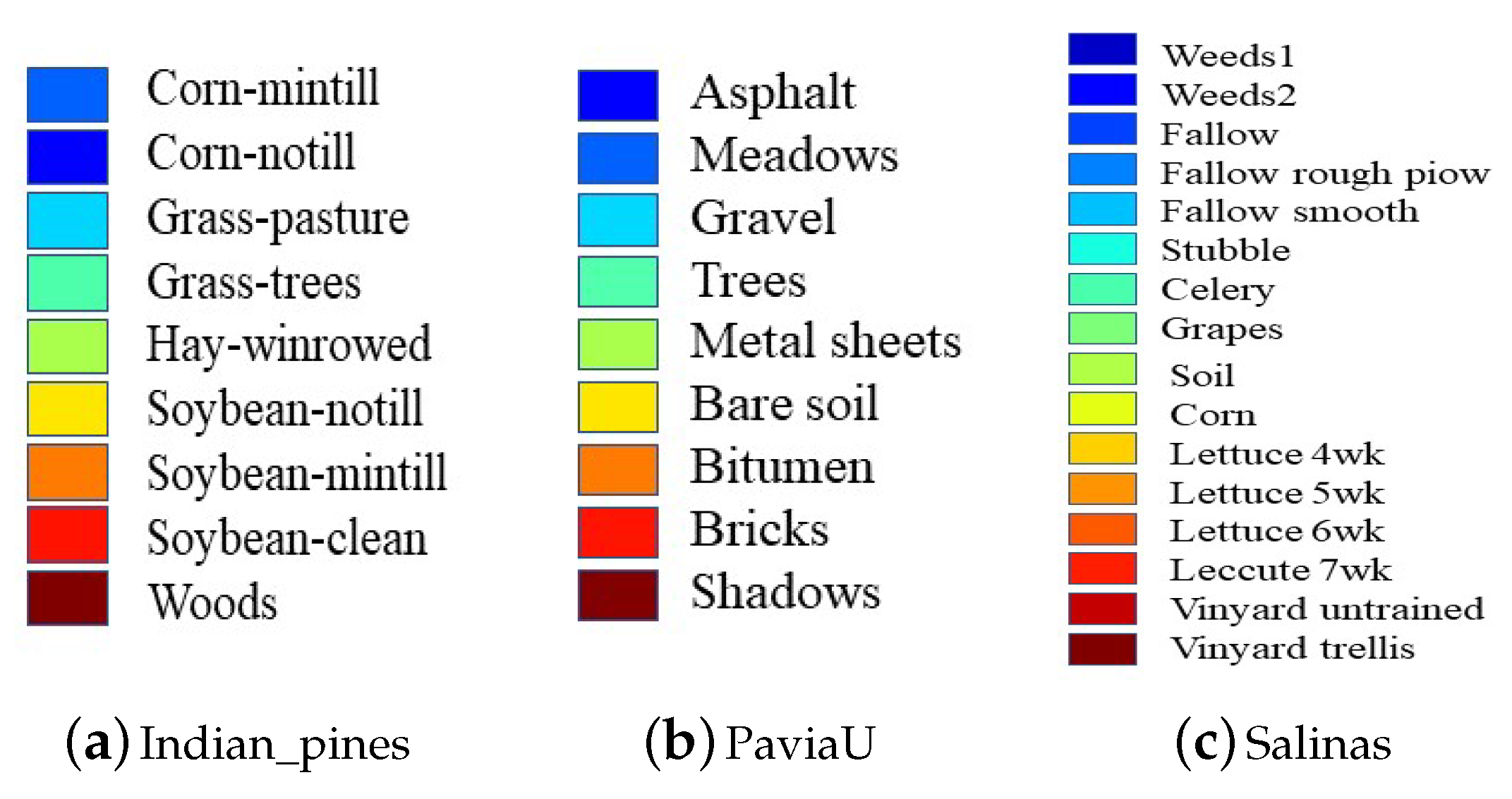
3.1. Dataset Description

We tested the proposed model and competing methods on three public HSI datasets, which are given as follows.

Indiana Pines Dataset: The Indiana Pines dataset was acquired by an Airborne Visible/Infrared Imaging Spectrometer (AVIRIS) sensor over the agricultural Indian Pine test site in the northwest of Indiana. Its spatial size is $145\times 145$, i.e., there are $145\times 145$ pixels in the Indiana Pines dataset, among which 10,366 pixels from 16 classes were labeled. As done in other works [40], we chose 9 out of 16 classes, which included 9234 labeled samples in total for the experiment. Each pixel had 220 bands ranging from 0.38 to 2.5 $\mathsf{\mu }$m. All bands were used in the experiment.

University of Pavia Dataset (PaviaU): PaviaU was acquired by the ROSIS sensor over the University of Pavia, Italy. Its spatial resolution is 1.3 m. There are $610\times 340$ pixels from 9 classes, among which 42,776 pixels were labeled and used for the experiment. Each pixel has 115 bands whose coverage ranges from 0.43 to 0.86 $\mathsf{\mu }$m. We discarded 12 water absorption bands and kept 103 bands in the experiment.

Salinas Scene Dataset: The Salinas scene dataset was also collected by the 224-band AVIRIS sensor over Salinas Valley, California. There are $512\times 217$ pixels, among which 54,129 pixels were labeled and used for the experiment. The water absorption bands were also discarded, and we kept 204 bands in the experiment.

3.2. Experimental Setup

We compared the proposed DCPN with k-NN, SVM, and several deep-learning-based methods, including the 1D-CNN [42], pixel-pair features(PPFs) based network [40], the 2D-CNN [41], and the 3D-CNN [45]. 1D-CNN is a pixel-level-based architecture. PPFs is a pixel-pair-based architecture. 2D-CNN [41] and 3D-CNN [45] are cube-based architectures. 3D-CNN is a truly 3D-structure-based method. Though 2D-CNN captures spatial and spectral information, it is a pesudo-3D CNN, since it treated the spatial information and spectral information, separately.

Before using these methods, we normalized the data first in order to guarantee the input value ranging from 0 to 1. The Libsvm toolbox was used to implement SVM, where radial basis kernel was adopted. All CNN-based methods were implemented via Tensorflow. For the proposed method, an Adam optimizer was used to minimize cross entropy, from which we obtained the parameters of the DCPN. The learning rate and the training epoch number (iteration number) of the proposed method was set to 0.001 and 100 in the experiments, respectively. Since the cube-pairs from Class 0 are much more than those from other classes, we selected only part of the cube-pairs from Class 0 to balance the data from different classes (see Section 2.2.2 for details). We set the spatial size of the cube and the extented-cube as $3\times 3$ and $5\times 5$, respectively. For a fair comparison, we set the spatial size to $3\times 3$ for those competing methods, which consider spatial information into account.

In this study, we chose overall accuracy (OA), which defines the ratio of correctly labeled samples to all test samples, to measure HSI classification results.

3.3. Comparison with Other Methods

In this section, we first chose 200 samples from each class as the training set and used the remaining samples for test. The number of training and test samples for each dataset can be seen from

Table 2. Training and test numbers for three datasets (Indiana Pines, PaviaU, and Salinas) used in this paper.

No.	Indiana Pines			PaviaU			Salinas
	Class Name	Train	Test	Class Name	Train	Test	Class Name	Train	Test
1	Corn-notill	200	1228	Asphalt	200	6431	Brocoli_1	200	1809
2	Corn-mintill	200	630	Meadows	200	18,449	Brocoli_2	200	3526
3	Grass-pasture	200	283	Gravel	200	1899	Fallow	200	1776
4	Grass-trees	200	530	Trees	200	2864	Fallow_plow	200	1194
5	Hay-win.	200	278	Sheets	200	1145	Fallow_smooth	200	2478
6	Soy.-notill	200	772	Bare Soil	200	4829	Stubble	200	3759
7	Soy.-mintill	200	2255	Bitumen	200	1130	Celery	200	3379
8	Soy.-clean	200	393	Bricks	200	3482	Grapes	200	11,071
9	Woods	200	1065	Shadows	200	747	Soil_vinyard	200	6003
10							Corn_weeds	200	3078
11							Lettuce_4wk	200	868
12							Lettuce_5wk	200	1727
13							Lettuce_6wk	200	716
14							Lettuce_7wk	200	870
15							Vinyard_un.	200	7068
16							Vinyard_ve.	200	1607
Sum		1800	7434		1800	40,976		3200	50,929

. We then conducted experiments, where the number of training sample varied.

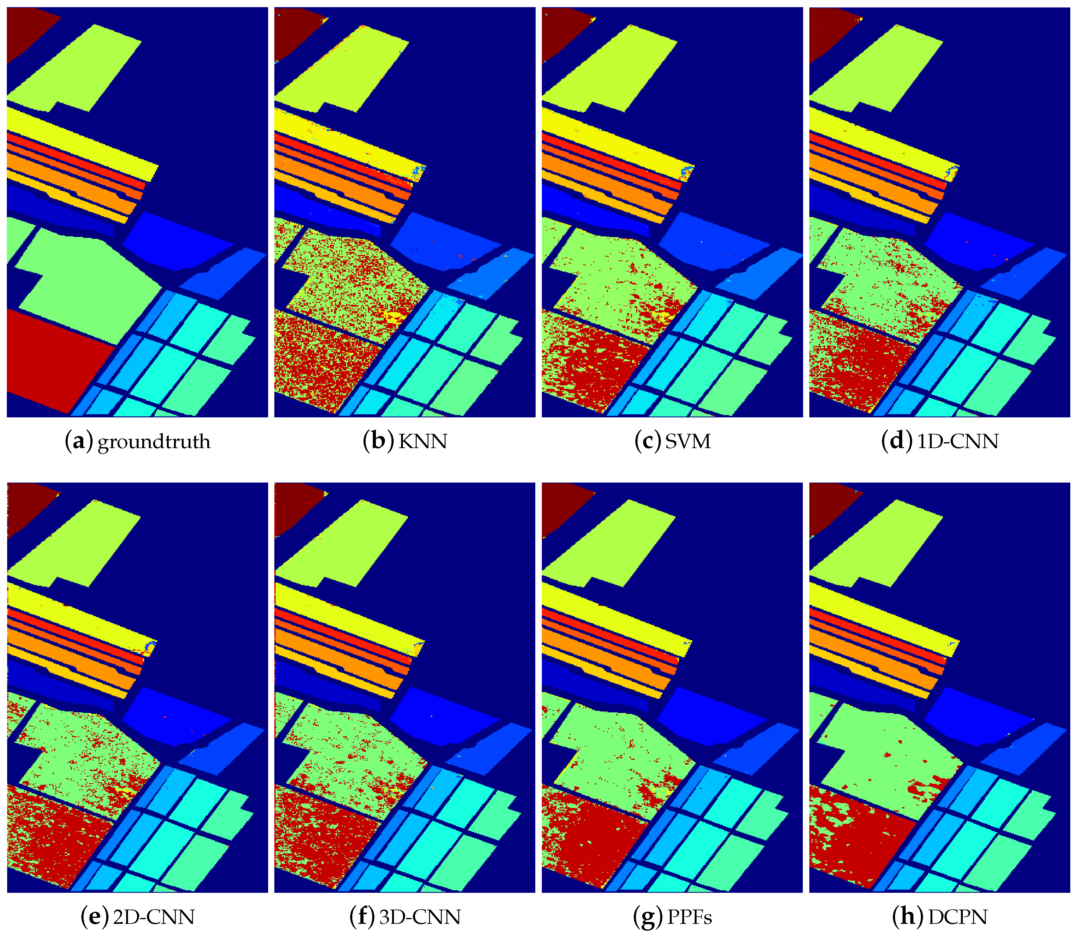
3.3.1. Experimental Results with 200 Training Samples

Given 200 training samples, the classification accuracies on three datasets are illustrated in

Table 3. Classification accuracy (%) of different methods on the Indiana Pines dataset.

No.	KNN	SVM	1D-CNN	2D-CNN	3D-CNN	PPFs	DCPN
1	63.07	80.92	74.56	84.53	83.70	92.99	95.32
2	61.38	85.10	59.34	74.70	73.06	96.66	98.55
3	91.52	96.61	84.21	89.42	93.01	98.58	99.68
4	98.81	99.06	95.07	98.44	98.82	100	99.87
5	99.46	99.68	98.58	99.89	99.75	100	100
6	74.70	86.76	65.06	74.15	76.49	96.26	97.91
7	51.74	74.17	84.66	92.33	93.92	87.80	94.42
8	57.18	89.24	66.27	78.99	76.19	98.98	98.93
9	92.66	98.62	98.77	99.56	99.33	99.81	99.86
OA	69.62	85.40	79.68	87.71	87.87	94.34	97.10

,

Table 4. Classification accuracy(%) of different methods on the PaviaU dataset.

No.	KNN	SVM	1D-CNN	2D-CNN	3D-CNN	PPFs	DCPN
1	75.45	86.35	94.32	97.84	97.80	97.42	98.95
2	76.51	92.38	95.38	96.71	98.06	95.76	98.24
3	76.94	86.08	60.14	84.68	82.01	94.05	97.19
4	92.21	96.76	74.96	91.68	91.49	97.52	97.81
5	99.38	99.65	99.07	98.57	99.77	100	100
6	76.54	92.35	68.66	83.82	85.02	99.13	98.94
7	92.12	93.95	56.51	91.02	82.12	96.19	98.99
8	76.12	86.44	75.05	90.71	90.03	93.62	98.87
9	99.95	99.99	99.01	99.27	99.92	99.60	99.75
OA	78.93	91.32	84.12	93.58	93.76	96.48	98.51

and

Table 5. Classification accuracy(%) of different methods on the Salinas dataset.

No.	KNN	SVM	1D-CNN	2D-CNN	3D-CNN	PPFs	DCPN
1	98.10	99.57	99.93	98.06	99.81	100	99.86
2	99.38	99.78	99.27	99.42	99.91	99.88	99.79
3	99.32	99.66	98.69	97.71	98.36	99.60	99.66
4	99.66	99.56	97.26	99.53	99.37	99.49	99.71
5	99.26	97.69	97.85	97.75	98.13	98.34	99.65
6	99.51	99.78	99.76	99.49	99.87	99.97	99.97
7	99.08	99.54	98.82	99.29	98.13	100	99.91
8	64.69	83.79	81.30	91.42	85.09	88.68	89.89
9	96.91	99.34	99.32	99.06	99.32	98.33	99.92
10	90.21	94.49	95.66	90.29	91.89	98.60	98.42
11	97.43	98.29	98.73	89.82	93.85	99.54	99.48
12	99.92	99.92	98.81	96.24	97.99	100	99.91
13	98.32	99.37	99.20	91.24	98.04	99.44	100
14	94.21	98.77	93.76	90.91	95.07	98.96	99.71
15	67.82	70.60	66.47	72.84	77.08	83.53	91.41
16	98.48	99.04	98.80	91.58	97.52	99.31	99.28
OA	86.26	91.68	89.80	91.69	92.30	94.80	96.39

. It can be seen that our method obtains the best classification results on all datasets compared with all competing methods, which demonstrates the effectiveness of the proposed method. Based on the experimental results, some observations are achieved as follows.

(1)

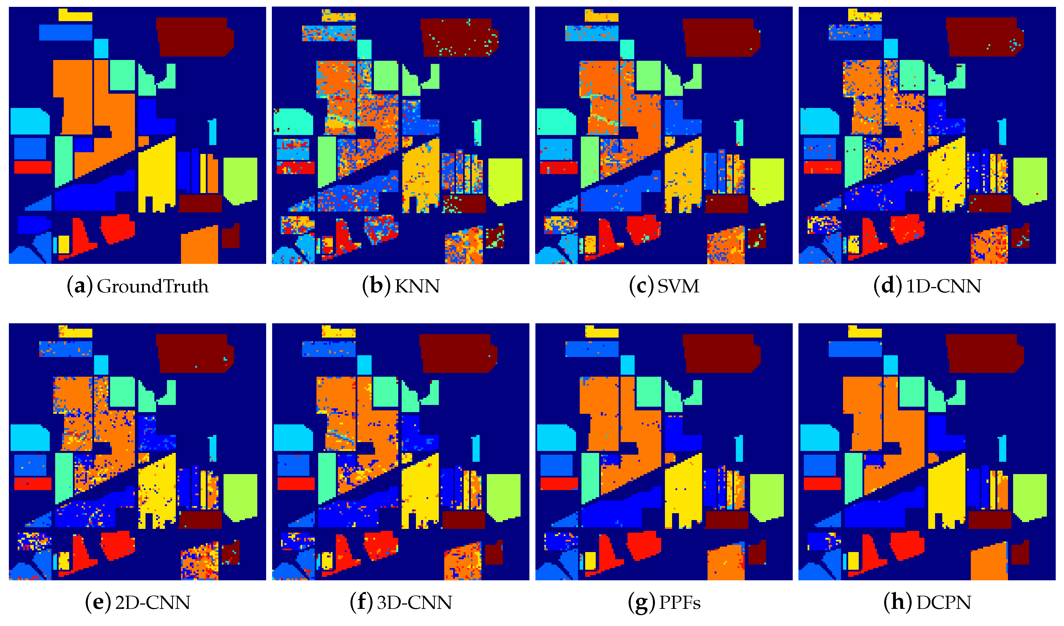
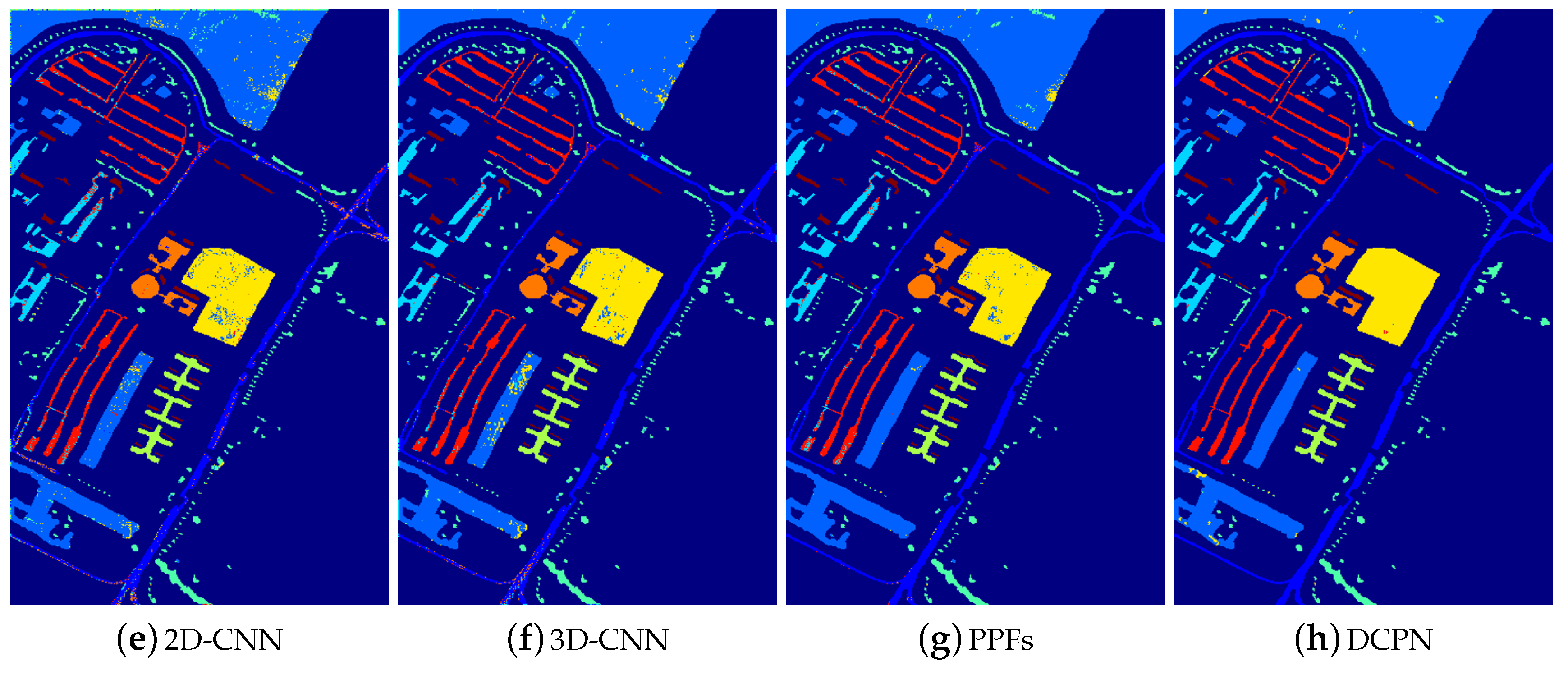
The majority of deep-learning-based methods have superior performance than the non-deep-learning-based HSI classification methods. Specifically, 2D-CNN, 3D-CNN, PPFs, and DCPN have superior performance than KNN and SVM. These experimental results verify the powerful capability of CNN-based methods for HSI classification.

(2)

Compared with the pixel-level-based CNN method, i.e., 1D-CNN, the proposed method improves the overall accuracy dramatically, e.g., 17.42% for the Indiana Pine dataset. Considering the difference between the proposed CNN architecture and pixel-level-based CNN architecture, we attribute the improvement mainly from the integration of 3D local structure and the cube-pair strategy.

(3)

It can be seen that pixel-pair-based method (i.e., PPFs) also improves the classification performance of HSI significantly, compared with the pixel-level-based method. This reflects the effectiveness of the pair-based strategy. However, the performance of PPFs inferiors to the proposed method, e.g., nearly 3% for the Indiana Pine dataset, which demonstrates that the local 3D structure is helpful to improve the HSI classification accuracy.

(4)

Though cube-based methods including 3D-CNN and 2D-CNN have superior performance than pixel-level-based methods, these methods are inferior to both the proposed method and the pixel-pair-based method. This phenomenon is caused by limited training samples, which makes 3D-CNN and 2D-CNN not well trained. Thus, it generalizes poorly on the test data. On the contrary, both cube-pair and pixel-pair strategies increase the training samples effectively, which guarantee that the network can be well trained.

Typical classification maps on three datasets are given in Figure 3, Figure 4 and Figure 5, where (a) represents the ground truth and (b)–(h) represent the classification maps from different methods. We use different colors to denote different categories in these figures, which are illustrated in Figure 6. We can see that the proposed method has the best classification results, which is consistent with the results analyzed above.

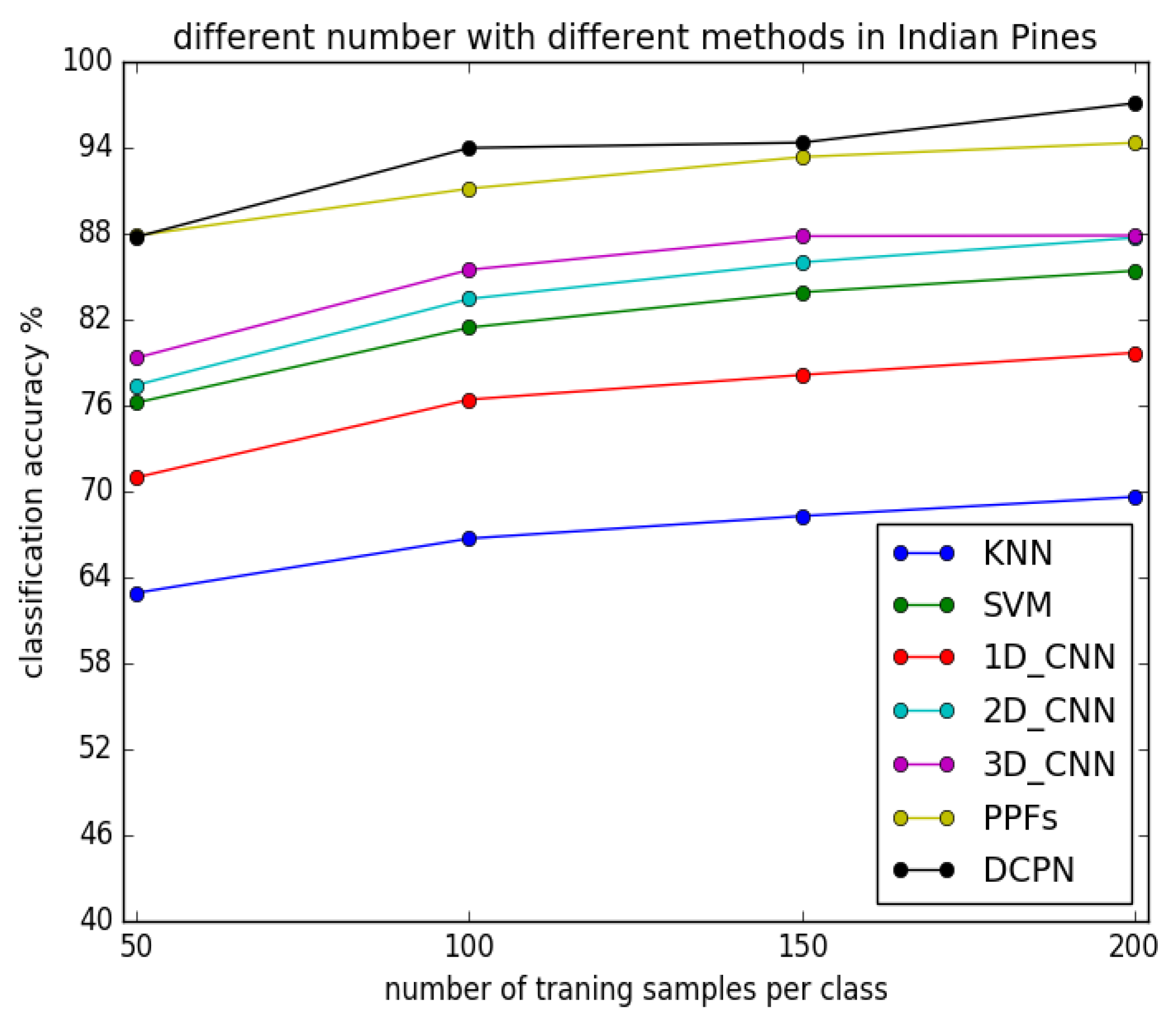
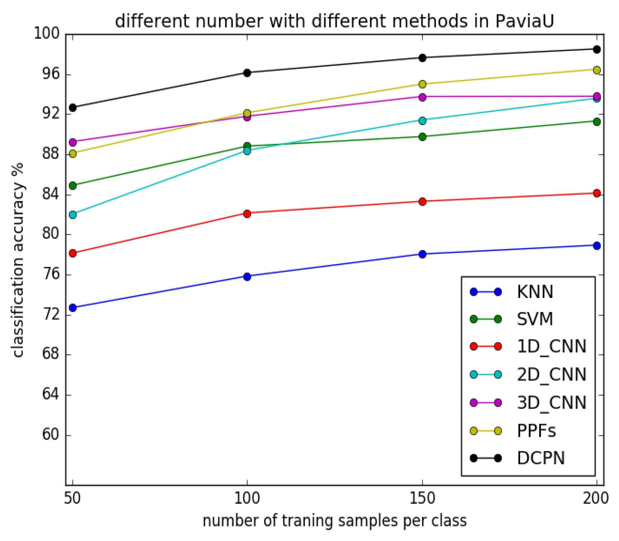
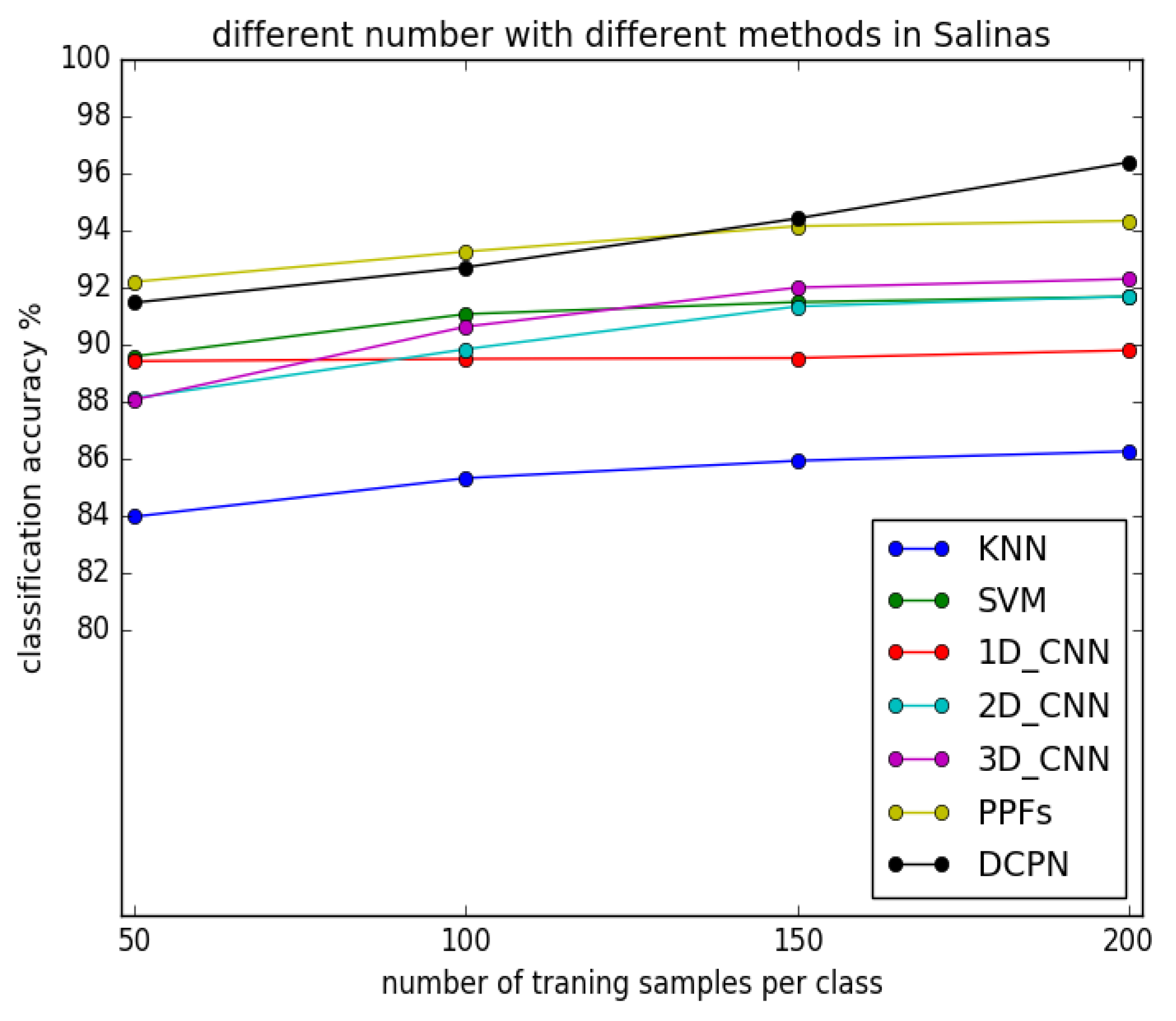
3.3.2. Experimental Results with Different Number of Training Samples

The classification results with different numbers of training samples are shown in Figure 7, Figure 8 and Figure 9, where the number varied from 50 to 200 with an interval of 50. From the experimental results, we can see the classification results of deep-learning-based methods increase when more samples are introduced for training, which is natural since the classifier can be well trained with more training samples. Nevertheless, the proposed method outperforms all competing methods stably given any amount of training samples.

From the above results, we can conclude that the proposed method has superior performance than any other competing methods.

3.4. Discussion

Considering that the cube size and layer number (i.e., depth) are two important parameters of the DCPN, to further testify the influence of these two parameters on classification results, the following two experiments are described and discussed.

In the first experiment, we fixed the layer number but set a different cube size. The experimental results on the Indiana Pines dataset can be seen in

Table 6. Classification accuracy with different cube sizes on the Indiana Pines dataset.

	k	1	3	5
ecs
3		94.45	/	/
5		94.71	96.18	/
7		95.57	97.10	96.16
9		/	97.04	96.88
11		/	/	97.21

, where $ecs$ denotes the size of the extended-cube and k denotes the size of the cube, respectively. It is noticeable that, when we set the cube size k as 1, the proposed method degenerates to a pixel-pair-based method. When we increase the cube size k from 1 to 3, the classification accuracy is also improved, which demonstrates local neighboring pixels are indeed helpful for classification. However, when we increase the cube size k further (e.g., from 3 to 5), the classification performance drops slightly. This phenomenon is caused by pixels from different categories, which are prone to be included with a larger cube size and decrease the classification accuracy. Thus, we set the size of cube k and extended-cube $ecs$ as 3 and 5, respectively, and fixed them in all experiments.

In the second experiment, we fixed the cube size but set a different layer number. The experimental results of the proposed DCPN and 3D-CNN on the Indiana Pines dataset can be seen in

Table 7. The classification accuracy with different layer numbers on the Indiana Pines dataset.

Layers	3	5	7	10
3D-CNN	87.87	83.61	77.79	75.86
DCPN	93.40	96.22	97.09	97.10

, where the layer number is chosen as 3, 5, 7, and 10. It can be seen that, with the increase in layer number, the classification accuracy of the DCPN improves, whereas the classification accuracy of 3D-CNN decreases. The comparison results are consistent with the above analysis. FCN has fewer parameters; thus, given the same amount of training samples, it can go deeper than CNN and has a superior nonlinear representation ablility.

4. Conclusions

In this paper, we propose a cube-pair-based HSI classification architecture. The proposed architecture can utilize the 3D characteristic of HSI and generalize well to the test data given only limited labeled training samples. Within this architecture, a 3D fully convolutional network is further modeled, which has fewer parameters than CNN. Thus, the proposed network has superior generalization ability compared with CNN when given the same amount of training samples. Experimental results on several HSI datasets demonstrate the proposed method has superior classification result compared with other state-of-the-art competing methods.

References

1. Ghamisi, P.; Yokoya, N.; Li, J.; Liao, W.; Liu, S.; Plaza, J.; Rasti, B.; Plaza, A. Advances in Hyperspectral Image and Signal Processing: A Comprehensive Overview of the State of the Art. IEEE Geosci. Remote Sens. Mag. 2018, 5, 37–78. [Google Scholar] [CrossRef]
2. Wei, W.; Zhang, L.; Tian, C.; Plaza, A.; Zhang, Y. Structured Sparse Coding-Based Hyperspectral Imagery Denoising With Intracluster Filtering. IEEE Trans. Geosc. Remote Sens. 2017, 55, 6860–6876. [Google Scholar] [CrossRef]
3. He, L.; Li, J.; Liu, C.; Li, S. Recent Advances on Spectral-Spatial Hyperspectral Image Classification: An Overview and New Guidelines. IEEE Trans. Geosci. Remote Sens. 2017, 56, 1579–1597. [Google Scholar] [CrossRef]
4. Guerra, R.; Barrios, Y.; Díaz, M.; Santos, L.; López, S.; Sarmiento, R. A New Algorithm for the On-Board Compression of Hyperspectral Images. Remote Sens. 2018, 10, 428. [Google Scholar] [CrossRef]
5. Fauvel, M.; Tarabalka, Y.; Benediktsson, J.A.; Chanussot, J.; Tilton, J.C. Advances in Spectral-Spatial Classification of Hyperspectral Images. Proc. IEEE 2013, 101, 652–675. [Google Scholar] [CrossRef]
6. Zhang, L.; Wei, W.; Shi, Q.; Shen, C.; Hengel, A.v.d.; Zhang, Y. Beyond Low Rank: A Data-Adaptive Tensor Completion Method. arXiv, 2017; arXiv:1708.01008. [Google Scholar]
7. Rasti, B.; Ghamisi, P.; Plaza, J.; Plaza, A. Fusion of Hyperspectral and LiDAR Data Using Sparse and Low-Rank Component Analysis. IEEE Trans. Geosci. Remote Sens. 2017, 55, 6354–6365. [Google Scholar] [CrossRef]
8. Zhang, L.; Wei, W.; Zhang, Y.; Shen, C.; van den Hengel, A.; Shi, Q. Cluster Sparsity Field: An Internal Hyperspectral Imagery Prior for Reconstruction. Int. J. Comput. Vis. 2018, 1–25. [Google Scholar] [CrossRef]
9. Lanaras, C.; Baltsavias, E.; Schindler, K. Hyperspectral Super-Resolution with Spectral Unmixing Constraints. Remote Sens. 2017, 9, 1196. [Google Scholar] [CrossRef]
10. Yang, J.; Zhao, Y.; Yi, C.; Chan, C.W. No-Reference Hyperspectral Image Quality Assessment via Quality-Sensitive Features Learning. Remote Sens. 2017, 9, 305. [Google Scholar] [CrossRef]
11. Transon, J.; d’Andrimont, R.; Maugnard, A.; Defourny, P. Survey of Hyperspectral Earth Observation Applications from Space in the Sentinel-2 Context. Remote Sens. 2018, 10, 157. [Google Scholar] [CrossRef]
12. Zhang, L.; Wei, W.; Zhang, Y.; Shen, C.; Hengel, A.V.D.; Shi, Q. Dictionary Learning for Promoting Structured Sparsity in Hyperspectral Compressive Sensing. IEEE Trans. Geosci. Remote Sens. 2016, 54, 7223–7235. [Google Scholar] [CrossRef]
13. Li, J.; Bioucas-Dias, J.M.; Plaza, A.; Liu, L. Robust Collaborative Nonnegative Matrix Factorization for Hyperspectral Unmixing. IEEE Trans. Geosci. Remote Sens. 2016, 54, 6076–6090. [Google Scholar] [CrossRef]
14. Zhang, L.; Wei, W.; Tian, C.; Li, F.; Zhang, Y. Exploring structured sparsity by a reweighted laplace prior for hyperspectral compressive sensing. IEEE Trans. Image Process. 2016, 25, 4974–4988. [Google Scholar] [CrossRef]
15. Ertürk, A.; Plaza, A. Informative Change Detection by Unmixing for Hyperspectral Images. IEEE Geosci. Remote Sens. Lett. 2017, 12, 1252–1256. [Google Scholar] [CrossRef]
16. Zhang, L.; Zhang, Y.; Yan, H.; Gao, Y.; Wei, W. Salient Object Detection in Hyperspectral Imagery using Multi-scale Spectral-Spatial Gradient. Neurocomputing 2018, 291, 215–225. [Google Scholar] [CrossRef]
17. Xue, J.; Zhao, Y.; Liao, W.; Kong, S.G. Joint Spatial and Spectral Low-Rank Regularization for Hyperspectral Image Denoising. IEEE Trans. Geosci. Remote Sens. 2018, 56, 1940–1958. [Google Scholar] [CrossRef]
18. Camps-Valls, G.; Bruzzone, L. Kernel-based methods for hyperspectral image classification. IEEE Trans. Geosci. Remote Sens. 2005, 43, 1351–1362. [Google Scholar] [CrossRef]
19. Wang, Q.; Lin, J.; Yuan, Y. Salient Band Selection for Hyperspectral Image Classification via Manifold Ranking. IEEE Trans. Neural Netw. Learn. Syst. 2016, 27, 1279. [Google Scholar] [CrossRef] [PubMed]
20. Rajadell, O.; García-Sevilla, P.; Pla, F. Spectral–Spatial Pixel Characterization Using Gabor Filters for Hyperspectral Image Classification. IEEE Geosci. Remote Sens. Lett. 2013, 10, 860–864. [Google Scholar] [CrossRef]
21. Wang, Q.; Meng, Z.; Li, X. Locality Adaptive Discriminant Analysis for Spectral–Spatial Classification of Hyperspectral Images. IEEE Geosci. Remote Sens. Lett. 2017, 14, 2077–2081. [Google Scholar] [CrossRef]
22. Ahmad, M.; Khan, A.M.; Hussain, R. Graph-based spatial–spectral feature learning for hyperspectral image classification. IET Image Process. 2017, 11, 1310–1316. [Google Scholar] [CrossRef]
23. Majdar, R.S.; Ghassemian, H. A probabilistic SVM approach for hyperspectral image classification using spectral and texture features. Int. J. Remote Sens. 2017, 38, 4265–4284. [Google Scholar] [CrossRef]
24. Samat, A.; Li, J.; Liu, S.; Du, P.; Miao, Z.; Luo, J. Improved hyperspectral image classification by active learning using pre-designed mixed pixels. Pattern Recognit. 2016, 51, 43–58. [Google Scholar] [CrossRef]
25. Medjahed, S.A.; Saadi, T.A.; Benyettou, A.; Ouali, M. Gray Wolf Optimizer for hyperspectral band selection. Appl. Soft Comput. 2016, 40, 178–186. [Google Scholar] [CrossRef]
26. Wang, Q.; Wan, J.; Yuan, Y. Locality Constraint Distance Metric Learning for Traffic Congestion Detection. Pattern Recognit. 2017, 75. [Google Scholar] [CrossRef]
27. Liu, L.; Wang, P.; Shen, C.; Wang, L.; Van Den Hengel, A.; Wang, C.; Shen, H.T. Compositional model based fisher vector coding for image classification. IEEE Trans. Pattern Anal. Mach. Intell. 2017, 39, 2335–2348. [Google Scholar] [CrossRef] [PubMed]
28. Blanzieri, E.; Melgani, F. Nearest Neighbor Classification of Remote Sensing Images With the Maximal Margin Principle. IEEE Trans. Geosci. Remote Sens. 2008, 46, 1804–1811. [Google Scholar] [CrossRef]
29. Ricardo, D.D.S.; Pedrini, H. Hyperspectral data classification improved by minimum spanning forests. J. Appl. Remote Sens. 2016, 10, 025007. [Google Scholar]
30. Guccione, P.; Mascolo, L.; Appice, A. Iterative Hyperspectral Image Classification Using Spectral–Spatial Relational Features. IEEE Trans. Geosci. Remote Sens. 2015, 53, 3615–3627. [Google Scholar] [CrossRef]
31. Li, J.; Bioucas-Dias, J.M.; Plaza, A. Spectral–Spatial Hyperspectral Image Segmentation Using Subspace Multinomial Logistic Regression and Markov Random Fields. IEEE Trans. Geosci. Remote Sens. 2012, 50, 809–823. [Google Scholar] [CrossRef]
32. Appice, A.; Guccione, P.; Malerba, D. Transductive hyperspectral image classification: toward integrating spectral and relational features via an iterative ensemble system. Mach. Learn. 2016, 103, 343–375. [Google Scholar] [CrossRef]
33. Melgani, F.; Bruzzone, L. Classification of hyperspectral remote sensing images with support vector machines. IEEE Trans. Geosci. Remote Sens. 2004, 42, 1778–1790. [Google Scholar] [CrossRef]
34. Sharma, S.; Buddhiraju, K.M. Spatial–spectral ant colony optimization for hyperspectral image classification. Int. J. Remote Sens. 2018, 39, 2702–2717. [Google Scholar] [CrossRef]
35. Lopatin, J.; Fassnacht, F.E.; Kattenborn, T.; Schmidtlein, S. Mapping plant species in mixed grassland communities using close range imaging spectroscopy. Remote Sens. Environ. 2017, 201, 12–23. [Google Scholar] [CrossRef]
36. Xue, Z.; Du, P.; Su, H. Harmonic Analysis for Hyperspectral Image Classification Integrated With PSO Optimized SVM. IEEE J. Sel. Top. Appl. Earth Obs. Remote Sens. 2014, 7, 2131–2146. [Google Scholar] [CrossRef]
37. Zabalza, J.; Ren, J.; Yang, M.; Zhang, Y.; Wang, J.; Marshall, S.; Han, J. Novel Folded-PCA for improved feature extraction and data reduction with hyperspectral imaging and SAR in remote sensing. ISPRS J. Photogramm. Remote Sens. 2014, 93, 112–122. [Google Scholar] [CrossRef] [Green Version]
38. Mura, M.D.; Villa, A.; Benediktsson, J.A.; Chanussot, J.; Bruzzone, L. Classification of Hyperspectral Images by Using Extended Morphological Attribute Profiles and Independent Component Analysis. IEEE Geosci. Remote Sens. Lett. 2011, 8, 542–546. [Google Scholar] [CrossRef]
39. Nielsen, A.A. Kernel Maximum Autocorrelation Factor and Minimum Noise Fraction Transformations. IEEE Trans. Image Process. 2011, 20, 612. [Google Scholar] [CrossRef] [PubMed]
40. Li, W.; Wu, G.; Zhang, F.; Du, Q. Hyperspectral Image Classification Using Deep Pixel-Pair Features. IEEE Trans. Geosci. Remote Sens. 2016, 55, 844–853. [Google Scholar] [CrossRef]
41. Zhang, H.; Li, Y.; Zhang, Y.; Shen, Q. Spectral-spatial classification of hyperspectral imagery using a dual-channel convolutional neural network. Remote Sens. Lett. 2017, 8, 438–447. [Google Scholar] [CrossRef]
42. Hu, W.; Huang, Y.; Wei, L.; Zhang, F.; Li, H. Deep Convolutional Neural Networks for Hyperspectral Image Classification. J. Sens. 2015, 2015, 258619. [Google Scholar] [CrossRef]
43. Wang, P.; Wu, Q.; Shen, C.; Dick, A.; Hengel, A.V.D. FVQA: Fact-based Visual Question Answering. IEEE Trans. Pattern Anal. Mach. Intell. 2017. [Google Scholar] [CrossRef] [PubMed]
44. Othman, E.; Bazi, Y.; Alajlan, N.; Alhichri, H.; Melgani, F. Using convolutional features and a sparse autoencoder for land-use scene classification. Int. J. Remote Sens. 2016, 37, 2149–2167. [Google Scholar] [CrossRef]
45. Li, Y.; Zhang, H.; Shen, Q. Spectral-Spatial Classification of Hyperspectral Imagery with 3D Convolutional Neural Network. Remote Sens. 2017, 9, 67. [Google Scholar] [CrossRef]
46. Slavkovikj, V.; Verstockt, S.; Neve, W.D.; Hoecke, S.V.; Walle, R.V.D. Hyperspectral Image Classification with Convolutional Neural Networks. In Proceedings of the Acm International Conference on Multimedia, Brisbane, Australia, 26–30 October 2015; pp. 1159–1162. [Google Scholar]
47. Chen, Y.; Jiang, H.; Li, C.; Jia, X.; Ghamisi, P. Deep Feature Extraction and Classification of Hyperspectral Images Based on Convolutional Neural Networks. IEEE Trans. Geosci. Remote Sens. 2016, 54, 6232–6251. [Google Scholar] [CrossRef]
48. Chen, Y.; Lin, Z.; Zhao, X.; Wang, G.; Gu, Y. Deep Learning-Based Classification of Hyperspectral Data. IEEE J. Sel. Top. Appl. Earth Obs. Remote Sens. 2017, 7, 2094–2107. [Google Scholar] [CrossRef]
49. Wang, P.; Cao, Y.; Shen, C.; Liu, L.; Shen, H.T. Temporal Pyramid Pooling-Based Convolutional Neural Network for Action Recognition. IEEE Trans. Circuits Syst. Video Technol. 2017, 27, 2613–2622. [Google Scholar] [CrossRef]
50. Zhang, X.; Liang, Y.; Li, C.; Ning, H.; Jiao, L.; Zhou, H. Recursive Autoencoders-Based Unsupervised Feature Learning for Hyperspectral Image Classification. IEEE Geosci. Remote Sens. Lett. 2017, 14, 1928–1932. [Google Scholar] [CrossRef]
51. Wang, C.; Zhang, L.; Wei, W.; Zhang, Y. When Low Rank Representation Based Hyperspectral Imagery Classification Meets Segmented Stacked Denoising Auto-Encoder Based Spatial-Spectral Feature. Remote Sens. 2018, 10, 284. [Google Scholar] [CrossRef]
52. Wang, Q.; Gao, J.; Yuan, Y. Embedding Structured Contour and Location Prior in Siamesed Fully Convolutional Networks for Road Detection. IEEE Trans. Intell. Transp. Syst. 2018, 19, 230–241. [Google Scholar] [CrossRef]
53. Zhong, P.; Gong, Z.; Li, S.; Schönlieb, C.B. Learning to Diversify Deep Belief Networks for Hyperspectral Image Classification. IEEE Trans. Geosci. Remote Sens. 2017, PP, 1–15. [Google Scholar] [CrossRef]
54. Chen, Y.; Zhao, X.; Jia, X. Spectral–Spatial Classification of Hyperspectral Data Based on Deep Belief Network. IEEE J. Sel. Top. Appl. Earth Obs. Remote Sens. 2015, 8, 2381–2392. [Google Scholar] [CrossRef]
55. Lin, M.; Chen, Q.; Yan, S. Network In Network. arXiv, 2013; arXiv:1312.4400. [Google Scholar]
Figure 1. Cube-pair-based convolutional neural network (CNN) classfication architecture.
Remotesensing 10 00783 g001
Figure 2. Structure of the proposed DCPN.
Remotesensing 10 00783 g002
Figure 3. Classification maps of different methods on the Indiana Pine dataset.
Remotesensing 10 00783 g003
Figure 4. Classification maps of different methods on the PaviaU dataset.
Remotesensing 10 00783 g004aRemotesensing 10 00783 g004b
Figure 5. Classification maps of different methods on the Salinas dataset.
Remotesensing 10 00783 g005
Figure 6. Colors represent different classes for three different datasets.
Remotesensing 10 00783 g006
Figure 7. Classification performance with different numbers of training samples on the Indiana Pines dataset.
Remotesensing 10 00783 g007
Figure 8. Classification performance with different numbers of training samples on the PaviaU dataset.
Remotesensing 10 00783 g008
Figure 9. Classification performance with different numbers of training samples on the Salinas dataset.
Remotesensing 10 00783 g009