Article

Bilateral Filter Regularized L2 Sparse Nonnegative Matrix Factorization for Hyperspectral Unmixing

1
High-Tech Institute of Xi’an, Xi’an 710025, China
2
School of Aerospace Science and Technology, Xidian University, Xi’an 710071, China
*
Author to whom correspondence should be addressed.
Remote Sens. 2018, 10(6), 816; https://doi.org/10.3390/rs10060816
Submission received: 11 April 2018 / Revised: 15 May 2018 / Accepted: 23 May 2018 / Published: 24 May 2018

Abstract

:
Hyperspectral unmixing (HU) is one of the most active hyperspectral image (HSI) processing research fields, which aims to identify the materials and their corresponding proportions in each HSI pixel. The extensions of the nonnegative matrix factorization (NMF) have been proved effective for HU, which usually uses the sparsity of abundances and the correlation between the pixels to alleviate the non-convex problem. However, the commonly used L 1 / 2 sparse constraint will introduce an additional local minima because of the non-convexity, and the correlation between the pixels is not fully utilized because of the separation of the spatial and structural information. To overcome these limitations, a novel bilateral filter regularized L 2 sparse NMF is proposed for HU. Firstly, the L 2 -norm is utilized in order to improve the sparsity of the abundance matrix. Secondly, a bilateral filter regularizer is adopted so as to explore both the spatial information and the manifold structure of the abundance maps. In addition, NeNMF is used to solve the object function in order to improve the convergence rate. The results of the simulated and real data experiments have demonstrated the advantage of the proposed method.

Graphical Abstract

1. Introduction

Hyperspectral imaging has become an emerging technique in remote sensing and has been successfully used in many applications, such as military reconnaissance, mineral exploration, and environmental monitoring [1]. Hyperspectral images (HSIs) record both the spatial and spectral information of a scene, and they can provide especially high spectral resolution with hundreds of narrow bands that enable precise material identification [2]. However, HSIs often suffer from low spatial resolution, which means that one pixel may contain more than one material; in other words, there are mixed pixels. To address this problem, the spectral information can be utilized to identify the spectrum of each material (called endmember) in the mixed pixels and their corresponding percentages (called abundance); the whole procedure is called unmixing. As a result of the widely existing mixed pixels in HSIs and in order to make full use of the data, it is important to develop efficient unmixing algorithms for HSI analysis.
There are two main categories of models for hyperspectral unmixing (HU), namely, the linear mixing model (LMM) and the nonlinear mixing model [3]. As a result of the model simplicity and good result interpretability, LMM-based approaches are predominant in the HU literature. Under the LMM, each mixed pixel is considered as a linear combination of endmember signatures that is weighted by the corresponding abundances. In addition, there are two constraints in the LMM that are used to obtain a physical meaning result, namely, the abundance nonnegative constraint (ANC) and the abundance sum-to-one constraint (ASC).
In the last decade, a large number of algorithms have been designed based on the LMM for HU [4]. These algorithms can be mainly divided into three categories, namely, geometrical, sparse regression based, and statistical. The geometrical unmixing algorithms are based on the fact that, under the LMM, the feature vectors of the pixels in HSI are all included in a simplex, and the vertices of the simplex are supposed as the endmembers. Some of the geometric based methods assume that pure pixels always exit in HSI, and the task of these algorithms is to search for these pure pixels as endmembers, including the pixel purity index [5], N-FINDER [6], automated morphological endmember extraction [7], vertex component analysis (VCA) [8], and the simplex growing algorithm [9]. Others do not depend on the pure pixel assumption and seek a minimum volume simplex that encloses the data set—for example, minimum volume enclosing simplex [10], simplex identification via variable splitting and augmented Lagrangian [11], and minimum volume simplex analysis [12]. Most of the geometric-based algorithms can only extract the endmembers. Hence, some abundance estimation algorithms are needed, such as the fully constrained least squares (FCLS) [13] and simplex projection unmixing [14]. The sparse regression-based algorithms work in a semi-supervised way, utilizing the ground spectral libraries so as to perform HU. An advantage of these approaches is that they evade the endmember extraction step and do not require the presence of pure pixels in the scene. However, they suffer from the large size of the spectral libraries and the difference between the ground library and the real measured data. The statistical approaches analyse the mixed pixels by exploiting the inner statistical rules in the data. These kinds of methods have been proven to be able to unmix highly mixed data and obtain a higher decomposition accuracy, despite the relatively high computation complexity. The representative algorithms of the statistical methods include the independent component analysis (ICA) [15,16], nonnegative matrix/tensor factorization (NMF/NTF) [17,18], and Bayesian approaches [19].
NMF focuses on the decomposition of a nonnegative matrix into two factors that are also nonnegative [20,21]. The non-negativity constraint makes the NMF-based algorithms particularly attractive, which allows for better interpretability. NMF-based algorithms have been successfully used over a variety of areas, such as document clustering, face recognition, blind audio source separation, and more. NMF has also shown great potential in HU. NMF-based unmixing algorithms estimate endmembers and abundances simultaneously and they satisfy the ANC in LMM naturally. However, the NMF problem is non-convex, and there are many local minima in the solution space. To alleviate this situation, extra auxiliary constraints are added upon the endmembers and abundances. Miao and Qi have proposed the minimum volume constrained NMF [22], which regulates the simplex volume that has been determined by the endmembers to be small. A similar idea is also adopted in the iterated constrained endmembers [23] and robust collaborative NMF [24], which replace the minimum volume constraint with a convex and simple surrogate. Huck introduced a regularizer that forces the endmember spectral variance to be low and thus encourages the flat endmember spectral, and proposed minimum dispersion constrained NMF [25]. The endmember dissimilarity constrained NMF [26] combines NMF with the endmember dissimilarity constraint, which can impose both a minimum volume and smoothing effects on endmembers.
The abundance constraints are also added into the NMF model in order to obtain a more accurate solution for HU. The sparsity of the abundance matrix is often considered under the fact that most of the pixels in HSI are mixed by only a subset of endmembers, rather than by all of the endmembers [27]. For example, the piecewise smoothness NMF with sparseness constraint [28], which was proposed by Jia and Qian, incorporates both the abundance smoothness and sparseness constraints into the NMF. Then, Qian et al. introduced the L 1 / 2 regularizer so as to enforce the sparsity of the abundances, and proposed the L 1 / 2 -NMF [29]. They demonstrated that the L 1 / 2 regularizer is a better choice because the ASC constraint and the L 1 regularizer are in conflict. The sparsity increases as q decreases for L q ( 1 / 2 q < 1 ), whereas the sparsity is not obviously improved as q continues to reduce for L q ( 0 < q 1 / 2 ). They also showed that the L 1 / 2 regularizer is closely linked to the minimum volume method, because when the volume of the simplex becomes larger, the sparse degree of the abundances becomes lower. Recently, some researchers have incorporated spatial information with the sparseness constraint. Zhu et al. has proposed a data-guided sparse method, in which the value of q for each pixel is determined by a learned data-guided map in order to adaptively impose the sparseness constraint [30]. A similar idea was adopted by Wang et al., as they incorporated a spatial group sparseness constraint into NMF for HU, which supposes that the pixels within a local spatial group share the same sparse structure [31].
The special information of the abundances is also a frequently exploited property in the literature for HU [32]. The ground objects usually change slowly, and each ground object often exists in a specific area of the whole scene. Based on these two facts, Liu et al. has proposed an approach that is named the abundance separation and smoothness constrained NMF (ASSNMF) [33], which imposes the abundance separation and smoothness constraints on NMF. Similarly, the total variation regularizer is introduced so as to promote the piecewise smoothness of the abundances in [34]. Moreover, some of the algorithms attempt to utilize the internal structural information of HSI and suppose that similar pixels correspond to similar abundances, such as graph-regularized L 1 / 2 -NMF (GLNMF) [35], structured sparse NMF (SS-NMF) [36], and hypergraph-regularized L 1 / 2 -NMF (HG L 1 / 2 -NMF) [37], which are all based on the graph Laplacian constraint [38]. In [39] and [40], however, the structural information is adopted by clustering and region segmentation, and the mean abundance of each class or region is computed so as to keep the abundance vectors similar.
In the existing unmixing algorithms, the abundance spatial or structural constraints are often used in conjunction with the sparsity constraints. In the commonly used sparsity constraints, the L 1 sparse constraint is no longer suitable when the ASC condition is needed, whereas the L 1 / 2 sparse constraint will introduce an additional local minima as a result of non-convexity, thereby reducing the algorithm convergence rate, and making it sensitive to noise. In most of the algorithms, the spatial and structural information are usually considered separately, so the correlation between the pixels is not fully utilized. In this paper, a new unmixing method, named the bilateral filter regularized L 2 sparse NMF (BF- L 2 SNMF), is proposed for HU. Two abundance constraints are added onto NMF. Firstly, the L 2 sparse constraint is proposed, which considers the sparseness of the abundance vectors. It can work when the ASC is satisfied, and has the attractive mathematical characteristics of simplicity and being Lipschitz continuous. Secondly, in order to make full use of the correlation between pixels in HSI, a graph constraint that is based on the bilateral filter is introduced. It considers the spatial information and the manifold structure features of the abundance maps together, which can effectively improve the accuracy of the endmember and abundance estimation. To improve the algorithm convergence rate, we used NeNMF to minimize the object function [41]. The main contributions of the paper are summarized as follows:
  • The L 2 sparse constraint is incorporated into the NMF model so as to improve the sparsity of the abundance vectors. In the case of satisfying the ASC condition, the L 2 sparse constraint can explore the sparse property of the abundance more effectively.
  • The bilateral filter regularizer is introduced so as to utilize the correlation information between the abundance vectors. By considering both the spatial and spectral distances between the pixels, the bilateral filter constraint can make the algorithm more adaptive to the regions that contain edges and complex texture.
The remainder of this paper consists of the following. In Section 2, the LMM and the NMF algorithm are briefly introduced. The proposed BF- L 2 SNMF model and its corresponding optimization solution are described in detail in Section 3. Section 4 presents and analyses the simulated and real data experiments for unmixing, using the BF- L 2 SNMF algorithm. Lastly, the discussions and conclusions are drawn in Section 5 and Section 6.

2. Background

In this section, we introduce the LMM and the NMF algorithm for subsequent discussion. The former is the basic model of the linear spectral unmixing, and the latter is one of the representative statistical methods for unmixing.

2.1. LMM

The LMM is the most popular model for HU. Many important developments in the field of HU are based on the LMM. Despite the fact that the LMM is not suitable in some specific strong nonlinear scenarios, it practically meets the needs of unmixing, in most cases. The LMM assumes that the endmembers do not interfere with each other, and thus each pixel in an HSI can be linearly represented by the endmembers.
x = A s + e
where A = [ a 1 , , a K ] + B × P is the endmember matrix that consists of P endmembers, and each column of A represents a type of endmember signal; B is the number of bands, s + P , which represents the abundance vector that is related to the pixel x + B ; and e B is the residual error and noise. If represented in matrix form, the HSI X B × N with N pixels can be described as follows:
X = A S + E
where S = [ s 1 , , s N ] + P × N is the abundance matrix, each column of S represents the abundance vector of a pixel, and every element in S is positive. E B × N is the residual item. Taking the ASC that has been mentioned previously into account, it is required to meet the following condition:
1 P T S = 1 N T
where 1 P T and 1 N T are full one-row vectors of lengths P and N , respectively. Since there are usually only a few endmembers in an HSI scene, and N is commonly large, we have P B N . It can be seen that the LMM-based HU is essentially a procedure for decomposing a high-dimension nonnegative matrix into two low-dimension nonnegative matrices, with the abundance matrix satisfying the ASC constraint extra, and on the basis of this, the results close to reality are encouraged.

2.2. NMF

NMF was proposed by Lee and Seung in 1999 [20], and it is widely used in the field of blind source separation. The goal of NMF is to approximately decompose a nonnegative matrix X + B × N into the form of X A S . Where A + B × P and S + P × N are all constrained to be nonnegative, and usually P min ( B , N ) . As a result of the nonnegative constraint, the NMF has a part-based representation [42], which makes the results more physically meaningful than other statistical methods, such as the principal component analysis and ICA. To solve the NMF problem, the object function is usually constructed as follows:
min A , S 1 2 X A S F 2 , s . t .   A 0 , S 0
where the approximate degree between X and A S is measured using the Euclidean distance, that is, the F-norm: F . Moreover, other similarity measures can also be used instead of the Euclidean distance, such as Kullback Leibler divergence or the Alpha and Beta divergence [17]. Since both A and S are unknown in Equation (4), the NMF problem is nonconvex and it is difficult to find the global minima. To minimize the object function, Lee and Seung have provided the sample and effective multiplication iterative algorithm [21]. The updated rules are as follows:
A A . X S T . / A S S T
S S . A T X . / A T A S
where ( ) T represents the transposition operation of a matrix, and . and . / represent the element-wise matrix multiplication and division operations, respectively. If A and S are initialized to be nonnegative, the updating formula can guarantee that they are always nonnegative during the iteration and it can converge. In addition, problem (4) can be solved by other methods, for example, the steepest gradient descent, Nesterov optimal gradient descent, and the Newton method [43].

3. Proposed Bilateral Filter Regularized L 2 Sparse NMF Method

As a result of the non-convexity of the NMF model, a lot of local minima existed in the solution space, so the optimization algorithm may have converged to a local optimum and the results were not unique for the different initializations. For example, given one solution of A and S , there existed a set of solutions, A D and D 1 S , which had the same reconstruction error, where D could be any nonnegative invertible matrix. In order to shrink the solution space, some effective constraints that reflected the intrinsic properties of HSI were usually added onto the NMF model. As we know, a pixel of HSI was usually composed by a small subset of the endmembers, so the abundance was often supposed to be sparse. Moreover, the correlation of the neighboring pixels was also reflected in abundance. In this paper, we proposed a NMF-based method, which combined the sparsity and correlation information of the abundance maps for HU.

3.1. L 2 Sparse Prior

Since most of the pixels were composed by only one or a few endmembers, but not all of the endmembers, the abundance vector of a pixel in HSI was usually assumed to be sparse. In other words, there were many zero entries in the abundance vector, and most of the entries of the abundance matrix were also supposed to be zero. Many solutions were proposed in order to exploit the abundance sparse property in recent years. The typical solution used the L 0 -norm regularizer by counting the nonzero elements in the abundance matrix. However, solving the L 0 -norm regularizer was an NP-hard problem, and the L 1 -norm regularizer was widely used as an alternative method. Although the L 1 -norm term could give a sparse solution in most cases, it could no longer play a role when the ASC was considered during the unmixing. Then, other alternative regularizers, such as the L p ( 0 < p < 1 )-norm regularizer and especially the L 1 / 2 -norm one, were proposed. The L p ( 0 < p < 1 )-norm minimization problem could be expressed as follows:
min s s 1 / p , s . t .    x = A s , s 0
Some additional techniques were introduced to further utilize the sparsity of the abundances more subtly, such as the data-guided sparsity [30], reweighted L 1 -norm regularizer [34], and the arctan sparse constraint [44]. In this paper, we considered the ASC and the sparse constraint together, and proposed to use the L 2 -norm in order to enhance the sparsity of the abundances in the NMF model.
We found that when the ASC condition was added, the larger the L 2 -norm of a pixel abundance vector, the sparser the abundance vector. For example, if there were two solutions s 0 = [ 0 , 1 , 0 ] T and s 1 = [ 1 / 3 , 1 / 3 , 1 / 3 ] T , the sparser solution s 0 had a larger L 2 -norm value. The L 2 -norm maximization problem could be summarized as follows:
max s s 2 , s . t .    x = A s , s 0 , 1 P T s = 1
where 2 represents the L 2 -norm of the vector. The L 2 sparse constraint had the advantages of simplicity and being Lipschitz continuous. It could get a relatively good sparse effect. The sparsity of the L 2 -norm under the ASC condition could be demonstrated by the following derivation. Assuming s = [ a , b , c ] T , and s met the ASC condition, that is a + b + c = 1 , and taking c = 1 a b into g ( s ) = s 2 2 , we get:
g ( s ) = 2 a 2 2 b 2 2 a b + 2 a + 2 b 1
Considering the sparseness of g ( s ) at a = 0 , we get the partial derivative of g ( s ) to a , as follows:
g ( s ) a | a = 0 = 2 ( 1 b )
Since b 1 , so g ( s ) / a 0 , if, and only if, b = 1 , the two sides were equal. Therefore, the L 2 -
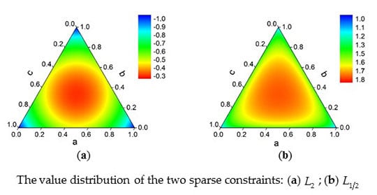
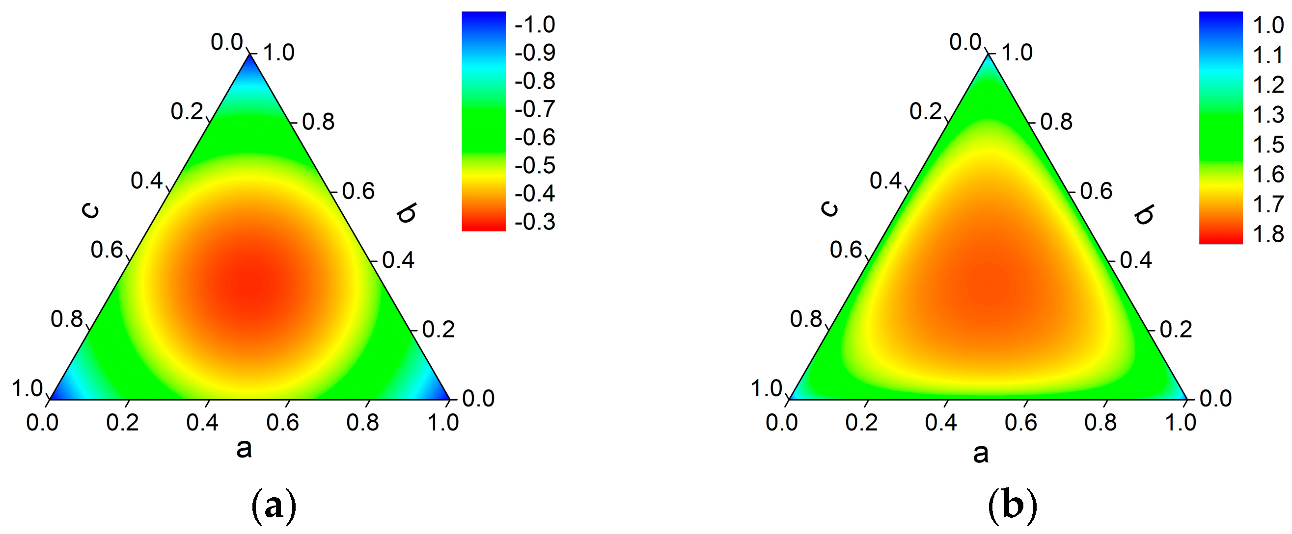
norm could have produced a certain sparse effect under the ASC condition. We plotted the value of g ( s ) as a triangle graph under the ASC condition, and we also plotted the function value of the L 1 / 2 constraint, which is h ( s ) = s 1 / 2 , as a comparison. As shown in Figure 1.
From Figure 1 we can see that as the sparsity of the abundance vector increased, the value of the L 2 sparse constraint decreased more uniformly than the L 1 / 2 constraint, which had a relatively big change, only when the sparsity was large. According to the analysis above, the L 2 sparse constraint was defined as follows:
min S J 1 ( S ) = 1 2 S F 2 , s . t . S 0 , 1 P T S = 1 N T
After adding the L 2 sparse constraint onto the NMF model, the new object function was shown in Equation (12), which we called L 2 sparse NMF ( L 2 SNMF).
min A , S 1 2 X A S F 2 + λ J 1 ( S ) , s . t . A 0 , S 0 , 1 P T S = 1 N T
In fact, similar to L 2 , the L p norm ( p > 1 ) could also make a sparse effect in the same way. In this paper, only the situation when p = 2 has been discussed.

3.2. Bilateral Filter Regularizer

The sparse constraint only considered the abundance characteristics of a single pixel. However, the pixels in HSI had correlations in both the spatial and spectral space. These correlations could have resulted in the similarities between some of the neighboring abundance vectors. Therefore, fully exploiting these correlations would have effectively improved the accuracy of the unmixing. When considering the correlation of the pixels in the spatial space, it was generally considered that the spatially adjacent pixels had similar abundance vectors, that is, the abundance map was smooth. Some algorithms were based on this assumption, such as ASSNMF. When considering the pixel correlation in the spectral space, the pixels with similar spectral features were considered to have similar abundance vectors, that is, the abundance vector data set maintained the manifold structure of the spectral feature data set. The algorithms that were based on this assumption included the GLNMF, SS-NMF, and HG L 1 / 2 -NMF. Inspired by the bilateral filter, we considered the correlations of the pixels in both the spatial and spectral space, and proposed a new regularizer that was based on the graph theory for hyperspectral unmixing, which we called the bilateral filter regularizer.
The bilateral filter was a simple and effective edge-preserving filter [45]. It took into account both the spatial and spectral similarity between pixels, and gave large weights to the pixels that were both spatially and spectrally similar. In the bilateral filter regularizer, we adopted a similar rule and supposed that the abundance vectors that corresponded to the pixels, which were both spatially and spectrally similar, had a higher degree of similarity. Given an HSI X + B × N , and considering each pixel in X as a node, the correlation weights between the different nodes could be learned as follows:
W i j = { ω i j , if   ω i j τ and   i j 0 , otherwise , ω i j = e d ( i , j ) 2 2 σ d 2 e x i x j 2 2 2 σ f 2
where d ( i , j ) represents the spatial distance between the i-th and the j-th pixels. We used the Euclidean distance. σ d is the distance diffusion parameter, σ f is the feature diffusion parameter, and ω i j is the joint similarity measure. Obviously, the larger the σ d , the smaller the effect of the spatial distance on ω i j , and the larger the σ f , the smaller the effect of the spectral distance on ω i j , and a large ω i j value suggests that the two pixels were similar. To better adapt to the edge area and the area where the features changed greatly, and to reduce the amount of computation, we set a threshold τ , and made ω i j effective only when the value of ω i j was greater than τ , otherwise we set the weight to 0. In this paper, we set τ to 0.1 (experience).
According to the process above, we could calculate the weight between any two pixels in the HSI and get the weight matrix W of size N × N . Under the previous assumption, similar pixels had similar abundance vectors. Using the L 2 -norm as the measure of distance, the bilateral filter regularizer that could control the level of similarity between the abundance vectors was defined as follows:
min S J 2 ( S ) = 1 2 i = 1 N j = 1 N W i j s i s j 2 2 = 1 2 Tr ( S D S T ) 1 2 Tr ( S W S T ) = 1 2 Tr ( S L S T ) , s . t . S 0
where Tr ( ) represents the trace of the matrix, D is a diagonal matrix and D i i = j W i j , and L = D W is generally called the graph Laplacian matrix.

3.3. The BF- L 2 SNMF Unmixing Model

By integrating the bilateral filter regularizer into L 2 SNMF Equation (12), the object function of the proposed BF- L 2 SNMF could be expressed as follows:
min A , S f ( A , S ) = 1 2 X A S F 2 + λ J 1 ( S ) + μ J 2 ( S ) , s . t . A 0 , S 0 , 1 K T S = 1 N T
In Equation (15), the first term was the reconstruction error, the second was used to enhance the sparseness of the abundance matrix, and the third was adopted to exploit the correlation between the abundance vectors.
There were two major improvements in BF- L 2 SNMF when compared with the other NMF-based unmixing algorithms. The first was the combination of the ASC constraint and the L 2 -norm so as to improve the sparsity of the abundance matrix. The second was the introduction of the bilateral filter regularizer that could better explore the pixel correlation information that was hidden in the HSI data.

3.4. Optimization Algorithm

Since both of the constraints in the BF- L 2 SNMF were Lipschitz continuous, NeNMF could be used to optimize the model. NeNMF was proposed by Guan et al. [41]. It used the Nesterov optimal gradient method to solve the NMF model, which had the advantage of a fast convergence rate, compared with the traditional multiplication iteration and the steepest gradient decent method. A strategy, named the alternating nonnegative least squares, was used to minimize the object function of Equation (15). For each iteration, one matrix was fixed, and the other was optimized, thus updating A and S alternately until convergence. We called this process the outer iteration. The first t + 1 outer iteration process was as follows:
A t + 1 = arg min A f ( A , S t ) S t + 1 = arg min S f ( A t + 1 , S )
When optimizing A , the alternating optimization method was also adopted in order to get the single optimal point. We called this process the inner iteration. According to the Nesterov optimal gradient method, which defined the auxiliary matrix A ¯ , the updating rules of A and A ¯ in the inner iteration could be expressed as follows:
A k = max ( 0 , A ¯ k 1 L A A f ( A ¯ k , S t ) )
α k + 1 = 1 + 4 α k 2 + 1 2
A ¯ k + 1 = A k + α k 1 α k + 1 ( A k A k 1 )
where α is the union coefficient, and max ( 0 , Z ) sets the negative value in matrix Z to 0, so that A satisfies the ANC. L A is the Lipschitz constant with respect to A , and for any two matrices, A 1 , A 2 B × P , L A should make the inequality of Equation (20) hold. We take L A as S t ( S t ) T 2 here.
A f ( A 1 , S t ) A f ( A 2 , S t ) F L A A 1 A 2 F
In this paper, the Karush–Kuhn–Tucker (KKT) conditions were used as the stopping criterion for the inner iteration. It was equal to the projection gradient of the object function to A , being 0. Since it was time consuming to completely converge to the extremely optimal point, we relaxed the stopping condition, and stopped the iteration when the F-norm of the projection gradient was less than a certain threshold, as follows:
A P f ( A k , S t ) F ε
where the threshold ε was set as 1e-3 in our experiments, and A P f ( A k , S t ) represents the projection gradient of the object function to A , which is defined as follows:
A P f ( A k , S t ) i j = { A f ( A k , S t ) i j ,                       ( A k ) i j > 0 min ( 0 , A f ( A k , S t ) i j ) , ( A k ) i j = 0
The whole process of optimizing A is shown in Algorithm 1.
Algorithm 1 Optimal gradient method (OGM)
Input: A t , S t
Output: A t + 1
1: Initialize A ¯ 0 = A t , α 0 = 1 , L A = S t ( S t ) T 2 , k = 0
repeat
  2: Using Equation (16), update A k
  3: Using Equation (17), update α k + 1
  4: Using Equation (18). update A ¯ k + 1
  5: k k + 1
until Stopping criterion is satisfied
6: A t + 1 = A t
In Algorithm 1, the solution of L A was similar to the method that was used in [41], and 2 was the spectral norm of the matrix. The gradient of the object function to A is as follows:
A f ( A , S ) = A S S T X S T
For updating the matrix S , we used the same method as A , except for the gradient and the Lipschitz constant. The gradient of the object function to S is as follows:
S f ( A , S ) = A T A S A T X λ S + μ S L
The solution of the Lipschitz constant, with respect to S , is shown in Equation (25), where S 1 , S 2 P × N . Since L may be a sparse matrix with large dimensions, it was difficult to solve the spectral norm. We used the F-norm instead.
S f ( A t , S 1 ) S f ( A t , S 2 ) F = ( A t ) T A t ( S 1 S 2 ) λ ( S 1 S 2 ) + μ ( S 1 S 2 ) L F ( A t ) T A t ( S 1 S 2 ) λ ( S 1 S 2 ) F + μ ( S 1 S 2 ) L F ( ( A t ) T A t λ I 2 + μ L F ) S 1 S 2 F
Therefore, the Lipschitz constant L S could be calculated as follows:
L S = ( A t ) T A t λ I 2 + μ L F
Using Algorithm 1 to optimize matrices A and S , we get the solution of BF- L 2 SNMF as Algorithm 2. We adopted the following stopping conditions for Algorithm 2, namely: (1) the number of iterations reached the maximum, and (2) the variation of the object function was less than a certain threshold for five continuous iterations. As long as one of the two conditions was satisfied, the iteration was terminated. In this paper, we set the maximum number of iterations to 200 and the stopping threshold to 1e-3.
To conveniently compare with other algorithms, we also provided the multiplication iteration method of L 2 SNMF. According to the gradient descent algorithm, we got the updating rule of BF- L 2 SNMF, as follows:
A t + 1 = A t u A A f ( A t , S t )
S t + 1 = S t u S S f ( A t + 1 , S t )
By setting μ = 0 , u A = A t . / A t S t ( S t ) T and u S = S t . / ( A t + 1 ) T A t + 1 S t , we got the updating rule of L 2 SNMF in multiplicative form, as follows:
A t + 1 = A t . X ( S t ) T . / A t S t ( S t ) T
S t + 1 = S t . ( ( A t + 1 ) T X + λ S t ) . / ( A t + 1 ) T A t + 1 S t
Algorithm 2 Bilateral Filter Regularized L 2 Sparse NMF (BF- L 2 SNMF) for HU
Input: Hyperspectral data X B × N ; the number of endmembers P ; the parameters λ , μ , σ d , σ f
Output: Endmember matrix A and abundance matrix S
1: Initialize A 1 , S 1 , and W
repeat
  2: Update A with A t + 1 = O G M ( A t , S t )
  3: Update S with S t + 1 = O G M ( A t + 1 , S t )
  4: t t + 1
until Stopping criterion is satisfied
5: A = A t , S = S t

3.5. Implementation Issues

Since the BF- L 2 SNMF algorithm was still non-convex, different initializations and parameters may have led to quite different results. During the implementation, there were several issues that needed attention.
The first issue was the initialization of A and S . Since there were many local minima in the solution space, the initialization of A and S was very important. There were many endmember initialization methods that were often used, such as the random initialization, artificial selection, K-means clustering, and some fast geometric endmember extraction algorithms. For the initialization of abundance, the common methods included the random initialization, project Moor–Penrose inverse, and FCLS. In this paper, we used the VCA and FCLS to initialize A and S in the simulation and the Cuprite data experiments, and we used the K-means clustering and the project Moor–Penrose inverse as the initializations in the urban data experiment.
The second issue was the ASC constraint. Since the proposed L 2 sparse constraint could produce the sparse effect only when the ASC condition was satisfied, the ASC constraint was necessary for the BF- L 2 SNMF. In some cases, where the ASC constraint was not suitable, we could replace the L 2 sparse constraint with the L 1 -norm. We considered the ASC constraint in the same way as [13]. When updating S during the iteration, X and A were replaced by X C and A C , which were defined as Equation (31). Where δ controlled the strength of the constraint, in this paper, we set δ to 20.
X C = [ X δ 1 T ] , A C = [ A δ 1 T ]
The third was the parameter determination. There were five parameters in BF- L 2 SNMF. They were P , λ , μ , σ d , and σ f . P was the number of endmembers, we assumed that P was known in this paper. In practice, some endmember number estimation algorithms, such as VD (virtual dimensionality) [46] or HySime [47], could have been used.
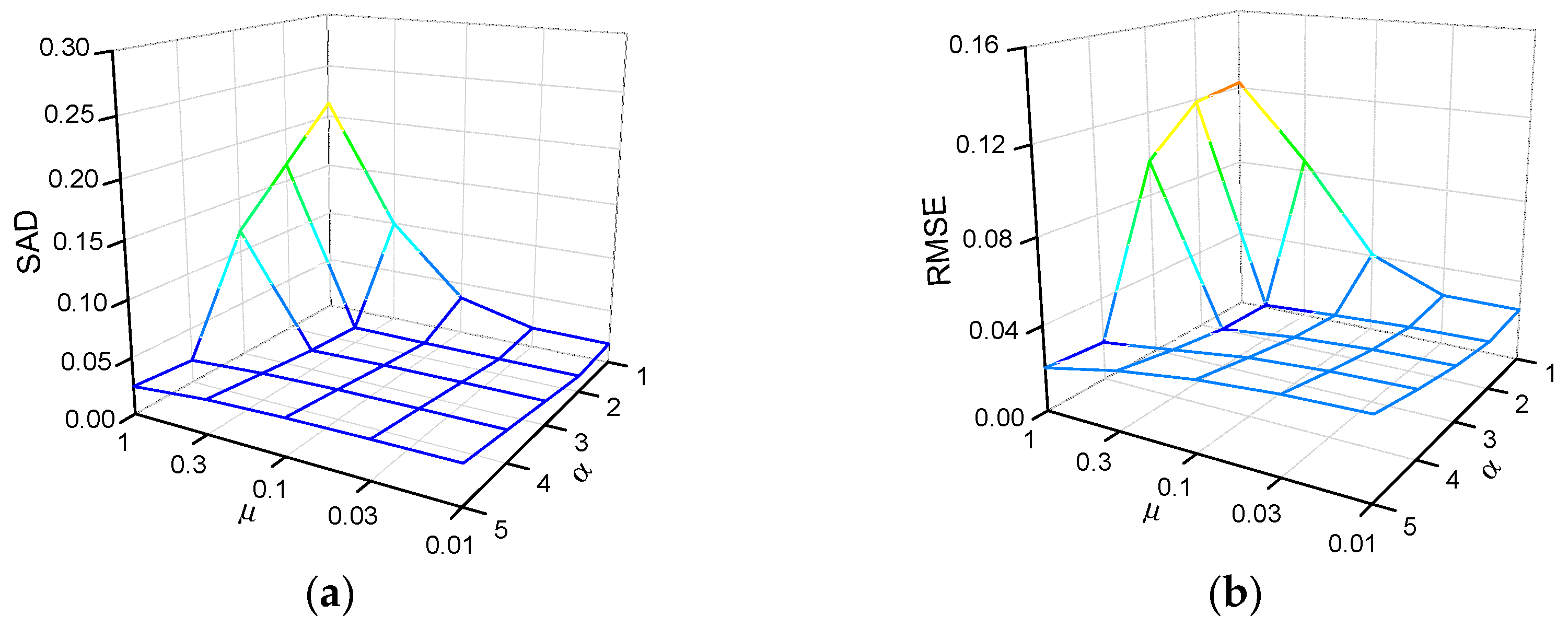
 λ and μ were the penalty coefficients, the choice of these two parameters should have been related to the sparsity and textural complexity of the image. We analyzed the impact of the different parameters on the results, with experiments in Section 4. σ d controlled the effective spatial range of the bilateral filter. We assumed that the area around pixel i , where pixel j satisfied exp ( d ( i , j ) 2 / 2 σ d 2 ) > τ as the valid spatial area. If the valid window size was set as 7 × 7 , then the value of σ d should have been in the range of [ 1.4 , 1.86 ] . In this paper, we selected σ d as 1.5. σ f controlled the effective spectral range. We expected to include the noise range in the effective spectral range exactly and to exclude the normal texture change. Based on this idea, we set σ f as the standard deviation of the image noise, and used the SVD (singular value decomposition) [48] method to estimate the noise.

3.6. Complexity Analysis

In this section, we analyzed the computational complexity of the BF- L 2 SNMF algorithm. The most time-consuming step in BF- L 2 SNMF was the calculation of A f ( A , S ) and S f ( A , S ) . Note that during the inner iteration, X S T , A T X , and the Lipschitz constant only needed to be calculated once. Since L was usually a sparse matrix, assuming the number of non-zero elements in L was C L , then the multiplication operation times for calculating S L were P C L . In addition, L F only needed to be calculated once in the whole algorithm, so it could have been calculated in the initialization process. Table 1 shows the number of multiplication operations in each iteration of BF- L 2 SNMF and that of the original NMF for comparison. Where K A and K S represented the inner iteration numbers of A and S , respectively. Moreover, learning the weight matrix W in advance was needed. The traditional bilateral filter algorithm was time-consuming, but some acceleration algorithms could be utilized, such as the recursive bilateral filter [49], whose computational complexity was O ( B N ) . For the whole algorithm procedure, assuming the number of outer iterations was m , the total computational complexity of NMF was O ( m B N P ) , whereas that of BF- L 2 SNMF was O ( m ( B N P + ( K A + K S ) P 2 ( B + N ) + P C L ) ) . For BF- L 2 SNMF, because of the fast convergence rate of the inner iteration, which was O ( 1 k 2 ) , K A and K S were generally small numbers. Therefore, the computational complexity of BF- L 2 SNMF was at the same level as that of the original NMF algorithm. However, because the BF- L 2 SNMF algorithm only required a few outer iterations, it consumed less time than the original NMF.

4. Experimental Results and Analysis

In order to verify the effectiveness of our algorithm, several experiments were conducted on simulated and real data. In these experiments, we compared the proposed BF- L 2 SNMF and L 2 SNMF with three other unmixing algorithms, namely, VCA-FCLS, L 1 / 2 -NMF, and GLNMF. We used the spectral angle distance (SAD) and the root mean square error (RMSE) to evaluate the extracted endmembers and abundances, respectively. SAD was utilized to evaluate the endmember estimation by calculating the angle between the estimated and the real endmembers, which was defined as follows:
SAD ( a ^ , a ) = arccos ( a ^ T a a ^ a )
RMSE was used to evaluate the accuracy of the abundance estimation by calculating the error between the estimated and the real abundance, which was defined as follows:
RMSE ( s ^ , s ) = 1 N i = 1 N ( s ^ i s i ) 2
From Equations (32) and (33), we can see that the smaller the SAD, the more similar the two endmembers were, and that the smaller the RMSE, the more accurate the estimated abundance was.

4.1. Simulated Data Experiments

In the synthetic experiments, we randomly selected 13 spectral signals as endmembers from the U.S. Geological Survey (USGS) spectral library [50]; each spectrum contained 224 bands. The spectral values represented the reflectivity of the corresponding material at a range of wavelengths, from 0.4 to 2.5 µm. There were 188 bands that were selected as valid, which were consistent with the subsequent Airborne Visible/Infrared Imaging Spectrometer (AVIRIS) Cuprite data experiment. Seven of these endmember signals are shown in Figure 2a. The synthetic data were generated in a similar way to [22]. Firstly, an image with a size of 64 × 64 was divided into several 8 × 8 blocks, each block was assigned a random material, and the abundance maps were initially generated. Next, to produce the mixed pixels, a 9 × 9 low-pass filter was utilized so as to filter each abundance map. In order to increase the level of mixing, the pixels whose abundance purity was greater than 0.8 were replaced by a mixture with 1 / P as the abundance of each endmember. The false-color image of an example of the synthetic data is shown in Figure 2b. To simulate the noise, which widely existed in the real HSI, a zero-mean Gaussian noise was added to the synthetic data. Simulation data with different noise levels were produced by controlling the signal-to-noise ratio (SNR) of the image. The SNR was defined as follows:
S N R = 10 log 10 E [ x T x ] E [ n T n ]
where x and n represent the original signal and the pixel noise, respectively, and E [ ] represents the mathematical expectation operation. Four experiments were conducted to analyze the impact of the parameter selection, noise level, endmember number, and image size on the performance of the proposed method. In the experiments, unless otherwise specified, the image size was generally set to 64 × 64 , the number of endmembers was set to seven, and the SNR was set to 25 dB. Except for the VCA-FCLS method, we used VCA to initialize the endmembers for all of the algorithms, and the FCLS to calculate the initial abundances. To further improve the initialization quality, we conducted 10 VCA-FCLS processes, and then selected the set of results with a minimum object function value as the initialization. Considering the random factors in the simulation, to better reflect the real performance of the algorithms, we repeated the experiment 10 times, and calculated the mean and standard deviation of the results as the final estimation. To exclude the influence of random factors in the algorithm comparisons, we used the same simulation data and initialization matrices for the experiments that had the same simulation parameters, but used different algorithms.

4.1.1. Parameter Selection

In this experiment, we analyzed the effect of the choice of parameters λ and μ on the experimental results. Considering that λ controlled the strength of the sparse constraint, we set its value to be related to the sparsity of the image. According to [51], the sparsity of the hyperspectral data X , could be expressed by the following:
s p a r s e n e s s = 1 B b = 1 B N x b 1 / x b 2 N 1
We tried to analyze the effect of parameter selection on the performance of BF- L 2 SNMF by changing the setting of λ and μ. We set λ as λ = αsparseness, where α ∈ [1, 5], and set μ as μ ∈ [0.01, 1]. Figure 3a shows the variation of SAD that was obtained by BF-L2 SNMF, with different combinations of λ and μ, and Figure 3b shows the RMSE results.
As seen from Figure 3, better results could be obtained when λ and μ were set at a suitable ratio. As μ increased, λ should have also increased correspondingly, otherwise it would have resulted in a larger estimation error. This indicated that spatial correlation constraints needed to be used under the premise of a sparse constraint. This also inspired us to set the appropriate value for λ first, and then set μ when setting the parameters. In the simulated data experiments, we set α to 3, and μ to 0.1.

4.1.2. Noise Robustness Analysis

In this experiment, we verified the robustness of our method to noise by changing the noise level of the simulation data. We generated an image every 5 dB, from 15 dB to 35 dB in SNR, and thereby obtained the simulation images for the different noise levels. Figure 4 shows the results of the experiment, where the histogram height represented the mean value, and the length of the error bar represented the standard deviation. We can see that BF-L2 SNMF achieved the best results on both SAD and RMSE. With the increasing of SNR, the advantage of BF- L 2 SNMF became more obvious. L 2 SNMF achieved the second best result, followed by GLNMF. The accuracy of GLNMF was generally better than L1/2-NMF, but when the SNR was set to 35 dB, the result of L1/2-NMF was better than the GLNMF. The VCA-FCLS obtained the worst result. Overall, the proposed method was robust to different levels of noise and could achieve better unmixing results.

4.1.3. Robustness Analysis of Endmember Number

In this experiment, the sensitivity of the proposed method to the number of endmembers was studied. We changed the number of endmembers from 3 to 13 in step 2, and generated a set of simulation images. The mean values and standard deviations of SAD and RMSE that were obtained from the experiment are shown in Figure 5. We can see that the overall results that were obtained by BF- L 2 SNMF were the best, but when the number of endmembers was 9 and 11, the results of L 2 SNMF were slightly better than BF- L 2 SNMF, in terms of RMSE. In all of the cases, the results that were obtained by the proposed methods were superior to the other three compared methods. The experiments showed that BF- L 2 SNMF had a stable performance for different numbers of endmembers.

4.1.4. Robustness Analysis of Image Size

In this experiment, we evaluated the performance of our algorithms for different image sizes. We generated 64 × 64, 96 × 96, 128 × 128, and 160 × 160 sized simulation images. Figure 6 shows the mean values and standard deviations for SAD and RMSE. It can be seen that BF-L2 SNMF achieved the best results on SAD and RMSE at different image sizes. For the NMF-based methods, as the size of the image increased, the SAD value slowly decreased, while the RMSE value stayed almost unchanged. This was because the increase of the pixel number was more beneficial to the endmember estimation. This experiment showed that the proposed method was robust for images of different sizes.

4.2. Real Data Experiments

Two remote sensing hyperspectral data sets were utilized for the real data experiments. One was the urban data that were collected by the Hyperspectral Digital Imagery Collection Experiment (HYDICE) sensor over an urban area at Copperas Cove, TX, U.S., and the other was the Cuprite data that were collected by AVIRIS over the Cuprite mining site, Nevada. All of these data sets could be downloaded on [52]. We chose these two data sets for two reasons. One was that they were both widely used for HU research, and their corresponding high-confidence ground truth results were demonstrated in many literature studies. The other was that the urban data could represent the situation of high spatial resolution and high sparsity, while the Cuprite data represented the situation of low spatial resolution and low sparsity. This was conducive to test the generalization ability of the proposed method. To fully exert the performance of the algorithms for the urban data set, we used the K-means clustering to initialize the endmembers and we used the project Moor–Penrose inverse to initialize the abundances. Whereas, for the Cuprite data set, the VCA-FCLS was used as the initialization method because the resolution of the urban data wa higher, and there were many outliers in the scene; thus, the VCA was prone to error estimation. Like the simulated data experiment, we repeated the experiment 10 times for each method, and used the same initialization matrices for the different methods.
HYDICE Urban Data Set: The original urban data contained 210 bands covering the wavelength range of 400–2500 nm. In this experiment, the noise bands and atmospheric absorption bands (bands 1–4, 76, 87, 101–111, 136–153, 198–210) were removed, leaving 162 bands for unmixing. Figure 7a shows the false-color image of the urban data. According to previous studies [29,33], there were six types of material in the scene. They wereasphalt, grass, trees, rooves, metal, and dirt. The reference abundance maps for these materials are shown in Figure 7b.
To evaluate the performance of the endmember estimation, we calculated the SAD value between the estimated endmember signal and the reference spectrum. Table 2 shows the SAD values and their standard deviations that were obtained by unmixing the urban data with different methods, and the best results have been shown in bold. We can see from Table 2 that the BF- L 2 SNMF obtained the best mean SAD result. The error that was obtained by the VCA method was the largest. The methods that utilized the correlation information between the pixels had a considerable promotion over the basic methods, such as BF- L 2 SNMF and GLNMF. Figure 8 shows the reference spectrum and the endmember signal that were extracted by BF- L 2 SNMF. Figure 9 shows the greyscale abundance maps corresponding to each of the estimated endmembers that were obtained by BF- L 2 SNMF. It was clear that the unmixing results were consistent with the reference endmembers and abundances in general, except for the metal.
AVIRIS Cuprite Data Set: The Cuprite data contained 224 bands that covered a wavelength range from 0.4–2.5 µm. A total of 187 effective bands remained after removing the low SNR bands. A region of 250 × 191 was cut out for the experiment, and the false-color image is shown in Figure 10a. The reference endmember spectra could be obtained in the USGS spectral library [50]. Figure 10b shows the reference mineral distribution of the region that was provided by the USGS in 1995. According to [8], a total of 12 minerals were selected as endmembers, which were as follows: Alunite, Andradite, Buddingtonite, Dumortierite, Kaolinite_1, Kaolinite_2, Muscovite, Montmorillonite, Nontronite, Pyrope, Sphene, and Chalcedony.
The SAD values and their standard deviations between the reference spectra and the estimated endmember signals that were obtained by different methods, are shown in Table 3. It could be seen that the BF- L 2 SNMF and L 2 SNMF achieved a higher accuracy than the other compared methods. However, the performances of the BF- L 2 SNMF and GLNMF were not obviously promoted over the L 2 SNMF and L 1 / 2 -NMF. This was mainly because of the high similarity and mixing degree of endmembers in the Cuprite data. Figure 11 shows the comparison of the endmember signal that was extracted by BF- L 2 SNMF and the USGS library spectrum. Figure 12 shows the greyscale abundance maps that were obtained by BF- L 2 SNMF. It could be seen that the estimated endmember signals were quite similar to the reference spectra, and the abundance maps correlated well with the reference map.

5. Discussion

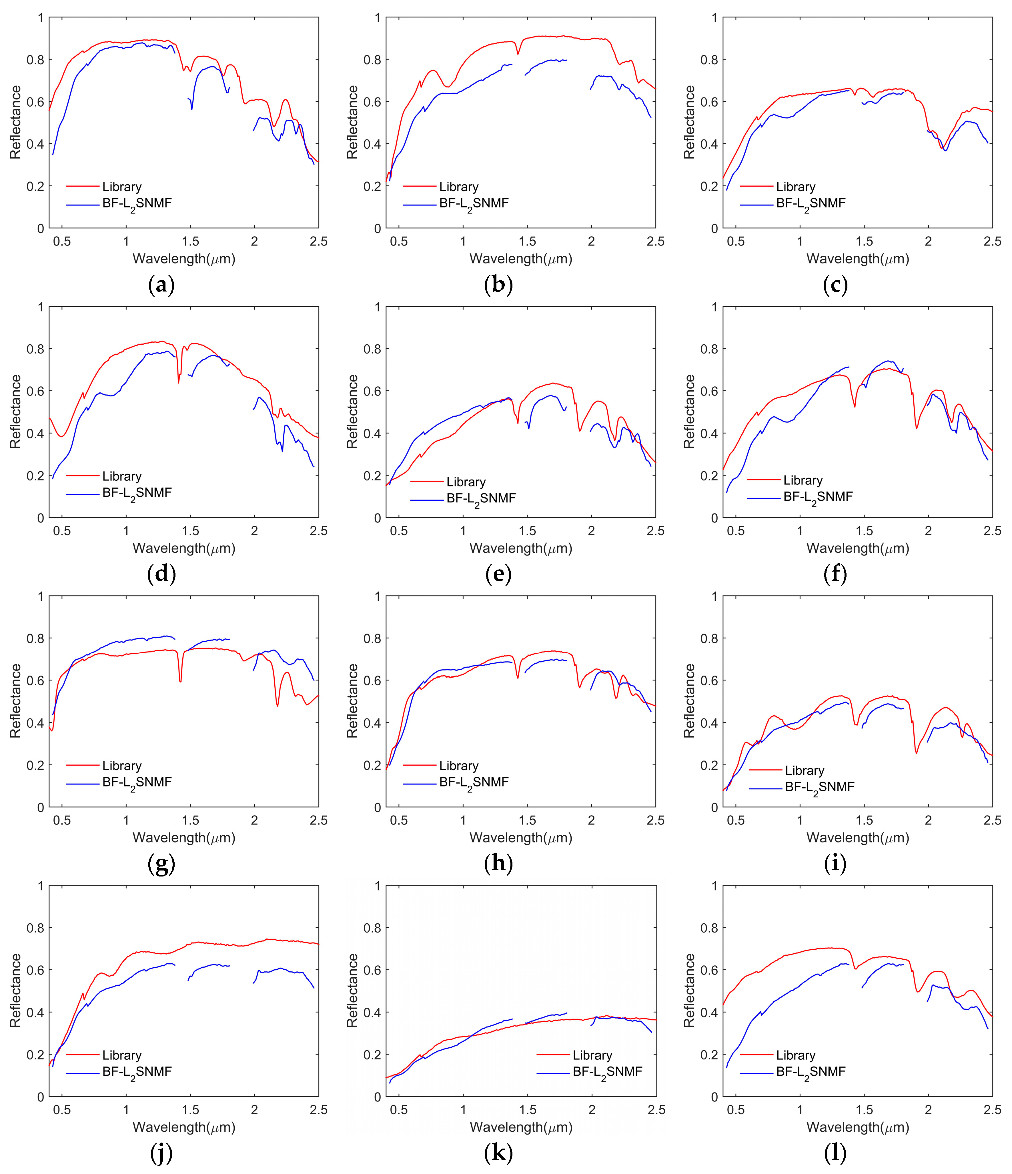
In this study, the validity of the BF- L 2 SNMF unmixing algorithm was investigated. The endmember signals and abundance maps that were estimated by the proposed BF- L 2 SNMF algorithm fitted well with the references. It could be seen from experiments in Section 4 that the performance of L 2 SNMF improved obviously when compared with L 1 / 2 -NMF. This demonstrated the advantage of the L 2 sparse constraint. The performance difference between BF- L 2 SNMF and L 2 SNMF was also bigger than that between GLNMF and L 1 / 2 -NMF. This indicated that the bilateral filter regularizer explored the correlation information between pixels more fully than the manifold regularizer in GLNMF. However, some improvements and issues need to be considered for further research.
Firstly, the BF- L 2 SNMF imposed the same sparse constraint for all of the pixels in HSI. However, the mixing level of each pixel or region might have been different from each other. The spatial information could be incorporated with the L 2 sparse constraint in order to achieve a more accuracy result. Similar to [30] and [31], a pixel-wise or region-smart L 2 sparse constraint might be developed.
Secondly, there were usually some regularization parameters that were to be set for the NMF-based unmixing methods. It was hard work to always set them with optimal values for different images. Although this paper had qualitatively analyzed the influence of the parameter choice on the results, it was still difficult to automatically determine the best values of λ and μ . Therefore, a trade-off should have be made. How to determine a set of relatively feasible λ and μ values adaptively might be a direction in future research.
Thirdly, the generalization ability of the proposed method needed further verification. Although two representative HSI data were selected for the real experiments, it could not be ensured that the algorithm was applicable to any scenario. More HSI data should be used to verify the effectiveness of the algorithm. As a result of the small amount of the public HSI data and reference, it was difficult to have a comprehensive inspection of the generalization ability for the algorithm. With the increasing of the public data set for HU, this issue might be solved in the future.

6. Conclusions

In this paper, a new algorithm, named the bilateral filter regularized L 2 sparse nonnegative matrix factorization (BF- L 2 SNMF), is developed for hyperspectral unmixing. The BF- L 2 SNMF model makes full use of two properties of the abundance maps in order to reduce the solution space of the original NMF model. The L 2 sparse constraint is proposed so as to exploit the sparse nature of the abundance maps. We have taken advantage of the fact that, under the abundance sum-to-one constraint, the stronger the sparsity of the abundance vector, the larger the L 2 -norm, and we have utilized the L 2 -norm as a measure of sparsity. In addition, a bilateral filter regularizer is employed to make full use of the correlation information between the pixels in the hyperspectral image. Both the spatial and spectral distance are considered to define the similarity measure of the abundance vectors. The simulated and real data experiments show that the proposed method can obtain a higher unmixing accuracy than the compared methods, which indicates that the adopted L 2 sparse constraint and bilateral filter regularizer in BF- L 2 SNMF are effective.

Author Contributions

All of the authors made significant contributions to the work. Z.Z. designed the research and analyzed the results. S.L. and Y.W. provided advice for the research and revised the paper. H.Z. and S.W. assisted in the preparation and validation work.

Acknowledgments

This work was supported, in part, by the National Natural Science Foundation of China under Grants 61673017 and 61403398.

Conflicts of Interest

The authors declare no conflict of interest.

References

  1. Ghamisi, P.; Yokoya, N.; Li, J.; Liao, W.; Liu, S.; Plaza, J.; Rasti, B.; Plaza, A. Advances in hyperspectral image and signal processing: A comprehensive overview of the state of the art. IEEE Geosci. Remote Sens. Mag. 2017, 5, 37–78. [Google Scholar] [CrossRef]
  2. Keshava, N.; Mustard, J.F. Spectral unmixing. IEEE Signal Process. Mag. 2002, 19, 44–57. [Google Scholar] [CrossRef]
  3. Ma, W.; Bioucas-Dias, J.M.; Chan, T.; Gillis, N.; Gader, P.; Plaza, A.; Ambikapathi, A.; Chi, C.-Y. A signal processing perspective on hyperspectral unmixing: Insights from remote sensing. IEEE Signal Process. Mag. 2014, 31, 67–81. [Google Scholar] [CrossRef]
  4. Bioucas-Dias, J.M.; Plaza, A.; Dobigeon, N.; Parente, M.; Du, Q.; Gader, P.; Chanussot, J. Hyperspectral unmixing overview: Geometrical, statistical, and sparse regression-based approaches. IEEE J. Sel. Top. Appl. Earth Obs. Remote Sens. 2012, 5, 354–379. [Google Scholar] [CrossRef]
  5. Boardman, J.W.; Kruscl, F.A.; Grccn, R.O. Mapping target signatures via partial unmixing of AVIRIS data. Summaries. In Proceedings of the JPL Airborne Earth Science Workshop, Pasadena, CA, USA, 23–26 January 1995; pp. 23–26. [Google Scholar]
  6. Winter, M.E. N-FINDR: An algorithm for fast autonomous spectral end-member determination in hyperspectral data. In Proceedings of the SPIE’s International Symposium on Optical Science, Engineering, and Instrumentation, Denver, CO, USA, 18–23 July 1999; pp. 266–275. [Google Scholar]
  7. Plaza, A.; Martínez, P.; Pérez, R.; Plaza, J. Spatial/spectral endmember extraction by multidimensional morphological operations. IEEE Trans. Geosci. Remote Sens. 2002, 40, 2025–2041. [Google Scholar] [CrossRef]
  8. Nascimento, J.M.; Bioucas-Dias, J.M. Vertex component analysis: A fast algorithm to unmix hyperspectral data. IEEE Trans. Geosci. Remote Sens. 2005, 43, 898–910. [Google Scholar] [CrossRef]
  9. Chang, C.; Wu, C.; Liu, W.; Ouyang, Y. A new growing method for simplex-based endmember extraction algorithm. IEEE Trans. Geosci. Remote Sens. 2006, 44, 2804–2819. [Google Scholar] [CrossRef]
  10. Chan, T.; Chi, C.; Huang, Y.; Ma, W. A convex analysis-based minimum-volume enclosing simplex algorithm for hyperspectral unmixing. IEEE Trans. Signal Process. 2009, 57, 4418–4432. [Google Scholar] [CrossRef]
  11. Bioucas-Dias, J.M. A variable splitting augmented Lagrangian approach to linear spectral unmixing. In Proceedings of the IEEE GRSS Workshop Hyperspectral Image Signal Processing: Evolution in Remote Sensing (WHISPERS), Grenoble, France, 26–28 August 2009; pp. 1–4. [Google Scholar]
  12. Li, J.; Agathos, A.; Zaharie, D.; Bioucas-Dias, J.M.; Plaza, A.; Li, X. Minimum Volume Simplex Analysis: A Fast Algorithm for Linear Hyperspectral Unmixing. IEEE Trans. Geosci. Remote Sens. 2015, 53, 5067–5082. [Google Scholar]
  13. Heinz, D.C.; Chang, C. Fully constrained least squares linear spectral mixture analysis method for material quantification in hyperspectral imagery. IEEE Trans. Geosci. Remote Sens. 2001, 39, 529–545. [Google Scholar] [CrossRef]
  14. Heylen, R.; Burazerovic, D.; Scheunders, P. Fully constrained least squares spectral unmixing by simplex projection. IEEE Trans. Geosci. Remote Sens. 2011, 49, 4112–4122. [Google Scholar] [CrossRef]
  15. Nascimento, J.M.; Dias, J.M. Does independent component analysis play a role in unmixing hyperspectral data? IEEE Trans. Geosci. Remote Sens. 2005, 43, 175–187. [Google Scholar] [CrossRef]
  16. Wang, N.; Du, B.; Zhang, L.; Zhang, L. An Abundance Characteristic-Based Independent Component Analysis for Hyperspectral Unmixing. IEEE Trans. Geosci. Remote Sens. 2015, 53, 416–428. [Google Scholar] [CrossRef]
  17. Cichocki, A.; Zdunek, R.; Phan, A.H.; Amari, S.I. Nonnegative Matrix and Tensor Factorizations: Applications to Exploratory Multi-Way Data Analysis and Blind Source Separation, 1st ed.; John Wiley & Sons Ltd.: Chichester, UK, 2009. [Google Scholar]
  18. Qian, Y.; Xiong, F.; Zeng, S.; Zhou, J.; Tang, Y.Y. Matrix-vector nonnegative tensor factorization for blind unmixing of hyperspectral imagery. IEEE Trans. Geosci. Remote Sens. 2017, 55, 1776–1792. [Google Scholar] [CrossRef]
  19. Dobigeon, N.; Moussaoui, S.; Coulon, M.; Tourneret, J.Y.; Hero, A.O. Joint Bayesian endmember extraction and linear unmixing for hyperspectral imagery. IEEE Trans. Signal Process. 2009, 57, 4355–4368. [Google Scholar] [CrossRef] [Green Version]
  20. Lee, D.D.; Seung, H.S. Learning the parts of objects by non-negative matrix factorization. Nature 1999, 401, 788–791. [Google Scholar] [PubMed]
  21. Lee, D.D.; Seung, H.S. Algorithms for non-negative matrix factorization. In Advances in Neural Information Processing Systems; MIT Press: Cambridge, MA, USA, 2001; pp. 556–562. [Google Scholar]
  22. Miao, L.; Qi, H. Endmember extraction from highly mixed data using minimum volume constrained nonnegative matrix factorization. IEEE Trans. Geosci. Remote Sens. 2007, 45, 765–777. [Google Scholar] [CrossRef]
  23. Berman, M.; Kiiveri, H.; Lagerstrom, R.; Ernst, A. Ice: A statistical approach to identifying endmembers in hyperspectral images. IEEE Trans. Geosci. Remote Sens. 2004, 42, 2085–2095. [Google Scholar] [CrossRef]
  24. Li, J.; Bioucas-Dias, J.M.; Plaza, A.; Liu, L. Robust collaborative nonnegative matrix factorization for hyperspectral unmixing. IEEE Trans. Geosci. Remote Sens. 2016, 54, 6076–6090. [Google Scholar] [CrossRef]
  25. Huck, A.; Guillaume, M.; Blanc-Talon, J. Minimum dispersion constrained nonnegative matrix factorization to unmix hyperspectral data. IEEE Trans. Geosci. Remote Sens. 2010, 48, 2590–2602. [Google Scholar] [CrossRef]
  26. Wang, N.; Du, B.; Zhang, L. An endmember dissimilarity constrained non-negative matrix factorization method for hyperspectral unmixing. IEEE J. Sel. Top. Appl. Earth Obs. Remote Sens. 2013, 6, 554–569. [Google Scholar] [CrossRef]
  27. Huang, R.; Li, X.; Zhao, L. Nonnegative matrix factorization with data-guided constraints for hyperspectral unmixing. Remote Sens. 2017, 9, 1074. [Google Scholar] [CrossRef]
  28. Jia, S.; Qian, Y. Constrained nonnegative matrix factorization for hyperspectral unmixing. IEEE Trans. Geosci. Remote Sens. 2009, 47, 161–173. [Google Scholar] [CrossRef]
  29. Qian, Y.; Jia, S.; Zhou, J.; Robles-Kelly, A. Hyperspectral unmixing via L1/2 sparsity-constrained nonnegative matrix factorization. IEEE Trans. Geosci. Remote Sens. 2011, 49, 4282–4297. [Google Scholar] [CrossRef]
  30. Zhu, F.; Wang, Y.; Fan, B.; Xiang, S.; Meng, G.; Pan, C. Spectral unmixing via data-guided sparsity. IEEE Trans. Image Process. 2014, 23, 5412–5427. [Google Scholar] [CrossRef] [PubMed]
  31. Wang, X.; Zhong, Y.; Zhang, L.; Xu, Y. Spatial group sparsity regularized nonnegative matrix factorization for hyperspectral unmixing. IEEE Trans. Geosci. Remote Sens. 2017, 55, 6287–6304. [Google Scholar] [CrossRef]
  32. Liu, R.; Du, B.; Zhang, L. Hyperspectral unmixing via double abundance characteristics constraints based NMF. Remote Sens. 2016, 8, 464. [Google Scholar] [CrossRef]
  33. Liu, X.; Xia, W.; Wang, B.; Zhang, L. An approach based on constrained nonnegative matrix factorization to unmix hyperspectral data. IEEE Trans. Geosci. Remote Sens. 2011, 49, 757–772. [Google Scholar] [CrossRef]
  34. He, W.; Zhang, H.; Zhang, L. Total variation regularized reweighted sparse nonnegative matrix factorization for hyperspectral unmixing. IEEE Trans. Geosci. Remote Sens. 2017, 55, 3909–3921. [Google Scholar] [CrossRef]
  35. Lu, X.; Wu, H.; Yuan, Y.; Yan, P.; Li, X. Manifold regularized sparse NMF for hyperspectral unmixing. IEEE Trans. Geosci. Remote Sens. 2013, 51, 2815–2826. [Google Scholar] [CrossRef]
  36. Zhu, F.; Wang, Y.; Xiang, S.; Fan, B.; Pan, C. Structured sparse method for hyperspectral unmixing. ISPRS J. Photogramm. Remote Sens. 2014, 88, 101–118. [Google Scholar] [CrossRef]
  37. Wang, W.; Qian, Y.; Tang, Y. Hypergraph-regularized sparse NMF for hyperspectral unmixing. IEEE J. Sel. Top. Appl. Earth Obs. Remote Sens. 2016, 9, 681–694. [Google Scholar] [CrossRef]
  38. Belkin, M.; Niyogi, P. Laplacian eigenmaps for dimensionality reduction and data representation. Neural Comput. 2003, 15, 1373–1396. [Google Scholar] [CrossRef]
  39. Lu, X.; Wu, H.; Yuan, Y. Double constrained NMF for hyperspectral unmixing. IEEE Trans. Geosci. Remote Sens. 2014, 52, 2746–2758. [Google Scholar] [CrossRef]
  40. Tong, L.; Zhou, J.; Li, X.; Qian, Y.; Gao, Y. Region-based structure preserving nonnegative matrix factorization for hyperspectral unmixing. IEEE J. Sel. Top. Appl. Earth Obs. Remote Sens. 2017, 10, 1575–1588. [Google Scholar] [CrossRef]
  41. Guan, N.; Tao, D.; Luo, Z.; Yuan, B. NeNMF: An optimal gradient method for nonnegative matrix factorization. IEEE Trans. Signal Process. 2012, 60, 2882–2898. [Google Scholar] [CrossRef]
  42. Gillis, N. The why and how of nonnegative matrix factorization. In Regularization, Optimization, Kernels, and Support Vector Machines, 1st ed.; Suykens, J.A.K., Signoretto, M., Argyriou, A., Eds.; Taylor & Francis: Boca Raton, FL, USA, 2014; pp. 257–291. [Google Scholar]
  43. Nesterov, Y. Introductory Lectures on Convex Optimization: A Basic Course, 1st ed.; Kluwer Academic: Boston, MA, USA, 2004. [Google Scholar]
  44. Salehani, Y.E.; Gazor, S. Smooth and sparse regularization for NMF hyperspectral unmixing. IEEE J. Sel. Top. Appl. Earth Obs. Remote Sens. 2017, 10, 3677–3692. [Google Scholar] [CrossRef]
  45. Tomasi, C.; Manduchi, R. Bilateral filtering for gray and color images. In Proceedings of the IEEE International Conference on Computer Vision (ICCV), Bombay, India, 4–7 January 1998; pp. 839–846. [Google Scholar]
  46. Chang, C.; Du, Q. Estimation of number of spectrally distinct signal sources in hyperspectral imagery. IEEE Trans. Geosci. Remote Sens. 2004, 42, 608–619. [Google Scholar] [CrossRef]
  47. Bioucas-Dias, J.M.; Nascimento, J.M. Hyperspectral subspace identification. IEEE Trans. Geosci. Remote Sens. 2008, 46, 2435–2445. [Google Scholar] [CrossRef]
  48. Scharf, L.L. Statistical Signal Processing, Detection Estimation and Time Series Analysis, 1st ed.; Addison-Wesley: Upper Saddle River, NJ, USA, 1991. [Google Scholar]
  49. Yang, Q. Recursive approximation of the bilateral filter. IEEE Trans. Image Process. 2015, 24, 1919–1927. [Google Scholar] [CrossRef] [PubMed]
  50. Clark, R.N.; Swayze, G.A.; Gallagher, A.J.; King, T.V.; Calvin, W.M. The US Geological Survey, Digital Spectral Library; Version 1 (0.2 to 3.0 µm); Technical Report; Geological Survey (US): Reston, VA, USA, 1993. [Google Scholar]
  51. Hoyer, P.O. Non-negative matrix factorization with sparseness constraints. J. Mach. Learn. Res. 2004, 5, 1457–1469. [Google Scholar]
  52. Zhu, F. Hyperspectral Unmixing Datasets & Ground Truths. Available online: http://www.escience.cn/people/feiyunZHU/Dataset_GT.html (accessed on 6 January 2018).
Figure 1. The value distribution of the two sparse constraints: (a) L 2 ; (b) L 1 / 2 .
Remotesensing 10 00816 g001
Figure 2. Example of the synthetic data: (a) endmember spectra and (b) false-color image.
Remotesensing 10 00816 g002
Figure 3. The experimental results for different parameters: (a) spectral angle distance (SAD) and (b) root mean square error (RMSE).
Remotesensing 10 00816 g003
Figure 4. The experimental results for different noise levels: (a) SAD and (b) RMSE.
Remotesensing 10 00816 g004
Figure 5. The experimental results for different endmember numbers: (a) SAD and (b) RMSE.
Remotesensing 10 00816 g005
Figure 6. The experimental results for different image sizes: (a) SAD and (b) RMSE.
Remotesensing 10 00816 g006
Figure 7. (a) False-color image of the Hyperspectral Digital Imagery Collection Experiment (HYDICE) urban data and (b) reference abundance maps of the urban data.
Remotesensing 10 00816 g007
Figure 8. The comparison of the reference spectrum and the estimated endmember signals obtained by BF- L 2 SNMF on the urban data set: (a) asphalt, (b) grass, (c) trees, (d) rooves, (e) metal, and (f) dirt.
Remotesensing 10 00816 g008
Figure 9. Abundance maps of endmembers estimated by BF- L 2 SNMF on the urban data set: (a) asphalt, (b) grass, (c) trees, (d) rooves, (e) metal, and (f) dirt.
Remotesensing 10 00816 g009
Figure 10. (a) Sub-image extracted from the Airborne Visible/Infrared Imaging Spectrometer (AVIRIS) Cuprite data and (b) reference map of the mineral distribution.
Remotesensing 10 00816 g010
Figure 11. The comparison of the U.S. Geological Survey (USGS) library spectrum and the estimated endmember signals obtained by BF- L 2 SNMF on the Cuprite data set: (a) Alunite, (b) Andradite, (c) Buddingtonite, (d) Dumortierite, (e) Kaolinite_1, (f) Kaolinite_2, (g) Muscovite, (h) Montmorillonite, (i) Nontronite, (j) Pyrope, (k) Sphene, and (l) Chalcedony.
Remotesensing 10 00816 g011
Figure 12. Abundance maps of endmembers estimated by BF- L 2 SNMF on the Cuprite data set: (a) Alunite, (b) Andradite, (c) Buddingtonite, (d) Dumortierite, (e) Kaolinite_1, (f) Kaolinite_2, (g) Muscovite, (h) Montmorillonite, (i) Nontronite, (j) Pyrope, (k) Sphene, and (l) Chalcedony.
Remotesensing 10 00816 g012aRemotesensing 10 00816 g012b
Table 1. Multiplication operation times in each iteration for nonnegative matrix factorization (NMF) and bilateral filter regularized L 2 sparse NMF (BF- L 2 SNMF).
AlgorithmMultiplication
NMF 2 B N P + 2 P 2 ( B + N ) + P ( B + N )
BF- L 2 SNMF 2 B N P + ( K A + K S + 1 ) P 2 ( B + N ) + P C L
Table 2. SAD values and their standard deviations (10−2) for different methods with the urban data. The best result in each row is shown in bold.
MethodBF- L 2 SNMF L 2 SNMFGLNMF L 1 / 2 -NMFVCA-FCLS
Asphalt0.1579 ± 6.830.1666 ± 9.510.1688 ± 7.040.2108 ± 8.480.3569 ± 25.86
Grass0.0758 ± 3.250.1613 ± 2.560.1399 ± 3.460.1777 ± 5.330.3425 ± 0.00
Tree0.1402 ± 2.520.1319 ± 3.870.1182 ± 3.310.1392 ± 5.440.4144 ± 20.85
Roof0.3271 ± 17.920.4495 ± 19.430.2830 ± 22.100.5036 ± 22.620.4371 ± 4.67
Metal0.3427 ± 10.170.4313 ± 33.860.6939 ± 22.570.5093 ± 29.240.5176 ± 20.44
Dirt0.0534 ± 2.070.0764 ± 2.450.0321 ± 0.580.0560 ± 2.011.1746 ± 0.70
Mean0.1829 ± 14.420.2362 ± 21.720.2393 ± 25.040.2661 ± 23.350.5405 ± 32.96
Table 3. SAD values and their standard deviations (10−2) for different methods on the Cuprite data. The best result in each row is shown in bold.
MethodBF- L 2 SNMF L 2 SNMFGLNMF L 1 / 2 -NMFVCA-FCLS
Alunite0.1480 ± 6.560.1385 ± 4.680.1294 ± 5.630.1285 ± 4.250.1678 ± 8.18
Andradite0.0755 ± 2.160.0811 ± 2.480.0788 ± 1.660.0970 ± 3.790.0715 ± 1.24
Buddingtonite0.1106 ± 1.410.0800 ± 1.810.0828 ± 0.960.0943 ± 1.670.0919 ± 2.16
Dumortierite0.0810 ± 1.600.0997 ± 1.650.1106 ± 1.690.0962 ± 1.680.0839 ± 1.84
Kaolinite_10.0831 ± 1.080.0887 ± 1.430.0916 ± 0.960.0777 ± 0.650.0900 ± 2.76
Kaolinite_20.0681 ± 2.170.0951 ± 2.100.0679 ± 2.790.0706 ± 1.970.0952 ± 2.83
Muscovite0.1432 ± 4.980.1458 ± 2.680.1418 ± 4.390.1308 ± 2.130.1458 ± 4.63
Montmorillonite0.0638 ± 0.870.0916 ± 3.370.0865 ± 2.410.0773 ± 1.650.0952 ± 2.58
Nontronite0.0836 ± 1.540.0768 ± 0.850.0842 ± 0.770.0810 ± 0.740.0748 ± 1.10
Pyrope0.0860 ± 3.640.0836 ± 3.950.0662 ± 0.840.0722 ± 2.280.1037 ± 4.45
Sphene0.0552 ± 0.670.0602 ± 0.550.0848 ± 1.590.1193 ± 6.640.0606 ± 1.57
Chalcedony0.1500 ± 1.470.1217 ± 3.220.1594 ± 4.020.1438 ± 3.000.1359 ± 2.84
Mean0.0957 ± 4.280.0969 ± 3.560.0987 ± 3.910.0991 ± 3.760.1013 ± 4.59

