Multilayer Perceptron Neural Network for Surface Water Extraction in Landsat 8 OLI Satellite Images
by
 ,
,
Wei Jiang
1,2 ,
,
Guojin He
1,3,4,*,
Tengfei Long
1,3,4,*,
Yuan Ni
1,5,
Huichan Liu
1,3,4,
Yan Peng
1,3,4,
Kenan Lv
1 and
Guizhou Wang
1,3,4 1
Institute of Remote Sensing and Digital Earth, Chinese Academy of Sciences, Beijing 100094, China
2
University of Chinese Academy of Sciences, Beijing 100049, China
3
Key Laboratory of Earth Observation Hainan Province, Sanya 572029, Hainan, China
4
Sanya Institute of Remote Sensing, Sanya 572029, Hainan, China
5
Key Laboratory of Spatial Data Mining & Information Sharing of Ministry of Education, Spatial Information Research Center of Fujian Province, Fuzhou University, Fuzhou 350002, China
*
Authors to whom correspondence should be addressed.
Remote Sens. 2018, 10(5), 755; https://doi.org/10.3390/rs10050755
Submission received: 25 March 2018
/
Revised: 7 May 2018
/
Accepted: 11 May 2018
/
Published: 15 May 2018
(This article belongs to the Special Issue Classification and Feature Extraction for Remote Sensing Image Analysis)
Abstract
:Surface water mapping is essential for monitoring climate change, water resources, ecosystem services and the hydrological cycle. In this study, we adopt a multilayer perceptron (MLP) neural network to identify surface water in Landsat 8 satellite images. To evaluate the performance of the proposed method when extracting surface water, eight images of typical regions are collected, and a water index and support vector machine are employed for comparison. Through visual inspection and a quantitative index, the performance of the proposed algorithm in terms of the entire scene classification, various surface water types and noise suppression is comprehensively compared with those of the water index and support vector machine. Moreover, band optimization, image preprocessing and a training sample for the proposed algorithm are analyzed and discussed. We find that (1) based on the quantitative evaluation, the performance of the surface water extraction for the entire scene when using the MLP is better than that when using the water index or support vector machine. The overall accuracy of the MLP ranges from 98.25–100%, and the kappa coefficients of the MLP range from 0.965–1. (2) The MLP can precisely extract various surface water types and effectively suppress noise caused by shadows and ice/snow. (3) The 1–7-band composite provides a better band optimization strategy for the proposed algorithm, and image preprocessing and high-quality training samples can benefit from the accuracy of the classification. In future studies, the automation and universality of the proposed algorithm can be further enhanced with the generation of training samples based on newly-released global surface water products. Therefore, this method has the potential to map surface water based on Landsat series images or other high-resolution images and can be implemented for global surface water mapping, which will help us better understand our changing planet.

1. Introduction
Water is the foundation that supports the survival of various biological activities in nature and is the basis for the production, life and development of social civilization [1,2]. In many types of water bodies, surface water, including lakes, rivers and reservoirs [3], plays an important role in Earth’s energy circulation and energy exchange [1], and it profoundly affects natural and human landscapes [4,5]. Surface water mapping has important practical significance and scientific value in terms of water resource management [1,6], biodiversity [7], disaster management [5,8] and climate change [9,10].
Remote sensing technology is an efficient and convenient mean for mapping global surface water at a large scale [11]. Different types of remote-sensing data (optical and radar) for surface water mapping have been widely documented [12,13]. In recent years, many scholars have conducted meaningful work on surface water mapping at a global scale, including the Global 3 arc-second Water Body Map (G3WBM) [9], the Global Land Cover Facility inland surface water map (GLCF-GIW) [3], the finer resolution observation and monitoring of the global land cover (FROM-GLC) water mask [14], the Global Land 30-water map [15] and high-resolution mapping of global surface water (HMGSW) [16]. These products are produced by combining a variety of water body extraction methods [15], which consist of four categories: the threshold method, the water index method, the object-oriented method and machine learning [15]. The threshold method extracts surface water using near-infrared or infrared bands [17]. The key to this method is determining the threshold between water and non-water bodies. Visually identifying this threshold may result in serious classification errors [18]; thus, automatic identification methods based on the differences in the gray value of a pixel have been used extensively to extract surface water [19]. The water index method is a popular method for highlighting surface water by establishing a water index, such as the normalized difference water index (NDWI) [20], the modified normalized difference water index (MNDWI) [21] and the automated water extraction index (AWEI) [22]. However, cloud shadows, mountain shadows, ice and snow remain major noise contributors when using the water index method [23]. The object-oriented method is typically utilized to extract surface water with a high-spatial-resolution remote image [24], such as ZY3 [25,26], SPOT5 [27], WorldView-2 [24] and WorldView-2 [28]. This method requires an enormous amount of time for image segmentation, and the efficiency of the extraction is limited [29]. The machine learning method is used to select tremendous amounts of training samples to identify surface water using different intelligent classifiers, including maximum likelihoods (MLs) [25], support vector machines (SVMs) [30], decision trees (DTs) [31], neural networks (NNs) [32] and constraint energy minimizations (CEMs) [33]. These methods are automatic, efficient and require less manual labor [15]. Although the machine learning method promotes global surface water mapping, there are still challenges regarding algorithm complexity and high-quality training samples [15].
Neural networks are a popular method used in target detections and image classifications across various image processing fields [34,35]. To solve complex situations, more layers are required in a neural network that has a full connection with all neurons, which is referred to as the multilayer perceptron (MLP) neural network [36]. However, with the deepening of neural network layers, the optimization function is likely to transform into a local optimal solution. As the new activation function emerges and the computer performance improves, an MLP with an increasing number of layers can be used in the field of image possessing by learning the spectral features at the pixel level. Compared with MLP, deep learning not only includes multiple layers, but it also has the ability to learn image shapes or texture features [37], such as the convolutional neural network (CNN) and the fully-convolutional network (FCN) [29,38]. For remote sensing images, the CNN and FCN have been widely applied in scene classifications [35,39], land cover classifications [40,41] and target detections [37] during recent years. Moreover, some studies have reported the application of the CNN or FCN in the surface water mapping community [29,42]. Yu et al. presented a novel CNN with a logistic regression to identify water via Landsat [42]. Furthermore, an FCN was proposed to map surface water by training a feature from a different land cover type [29]. Because the CNN or FCN conduct convolution computation during the process of model training, these methods are time consuming.
Multilayer perceptron neural networks have been verified to be an excellent neural network algorithm at the pixel level given the connection with perceptron [36], which has been employed to generate cloud masking [36], image classifications [43] and change detections [44] in the field of remote sensing. However, the application of MLP to surface water extraction has not been presented so far in the literature. Given this motivation, the purpose of this paper is to introduce MLP neural networks to extract surface water. To objectively illustrate the ability and performance of MLP in surface water extraction, the experiment is conducted at a large scale, and the applicability of the algorithm for different water and noise types is comprehensively compared. First, eight images covering different water types and water noises are collected as the experimental dataset. Subsequently, a water index and support vector machine are employed to compare the performance of the proposed algorithm for surface water mapping with previous methods. Then, the reliability of the proposed algorithm when suppressing noise (including cloud shadows, mountain shadows, building shadows and ice/snow) is verified. Finally, the band optimization, image preprocessing and training samples are analyzed and discussed. Through a comprehensive comparison and analysis, the proposed algorithm holds promise for mapping global surface water and helps us understand our changing planet in regard to global change.
2. Materials and Methods
2.1. Study Area and Dataset
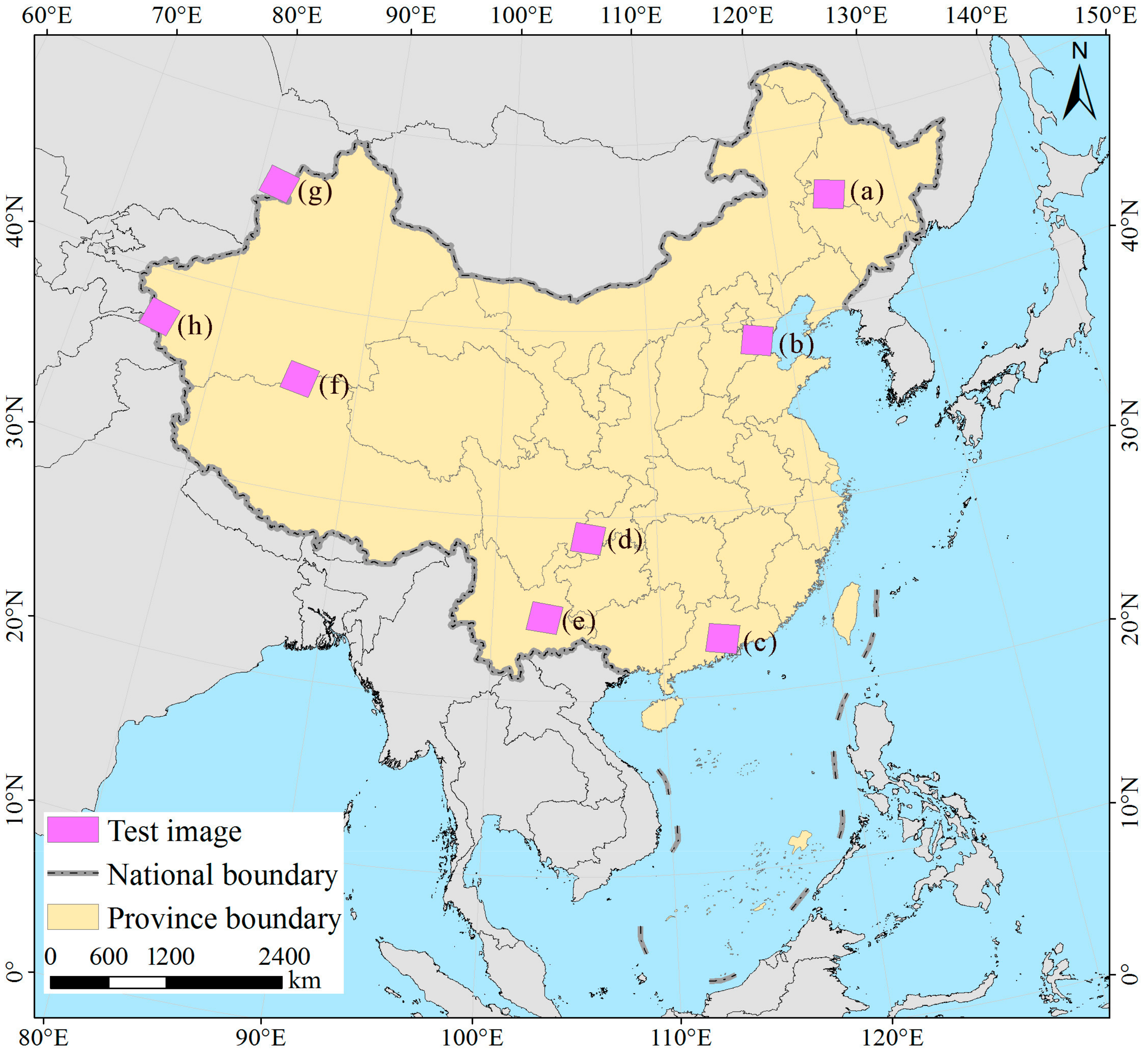
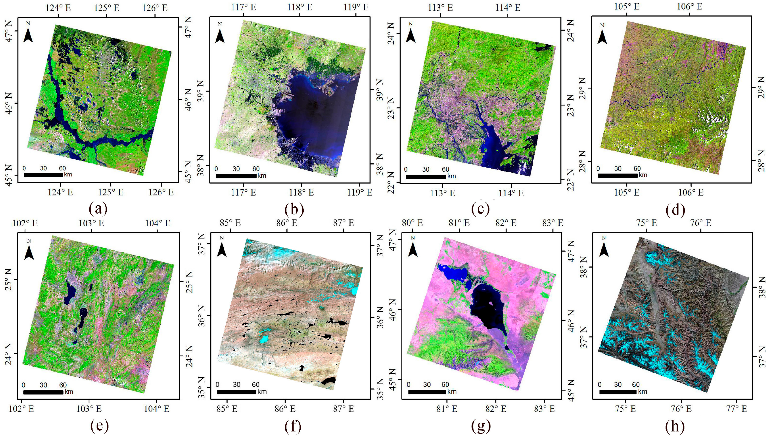
Different types of surface water are abundant in China, and eight typical regions are selected as the study area (Figure 1), which covers different surface water types, as shown in Table 1. The Landsat 8 OLI images (Figure 2) corresponding to the study areas are collected from the U.S. Geological Survey [45], and the metadata information of these images are shown in Table 1. In addition, major noise from cloud shadows, mountain shadows, building shadows and snow/ice are also included in the collected dataset.
2.2. Methods
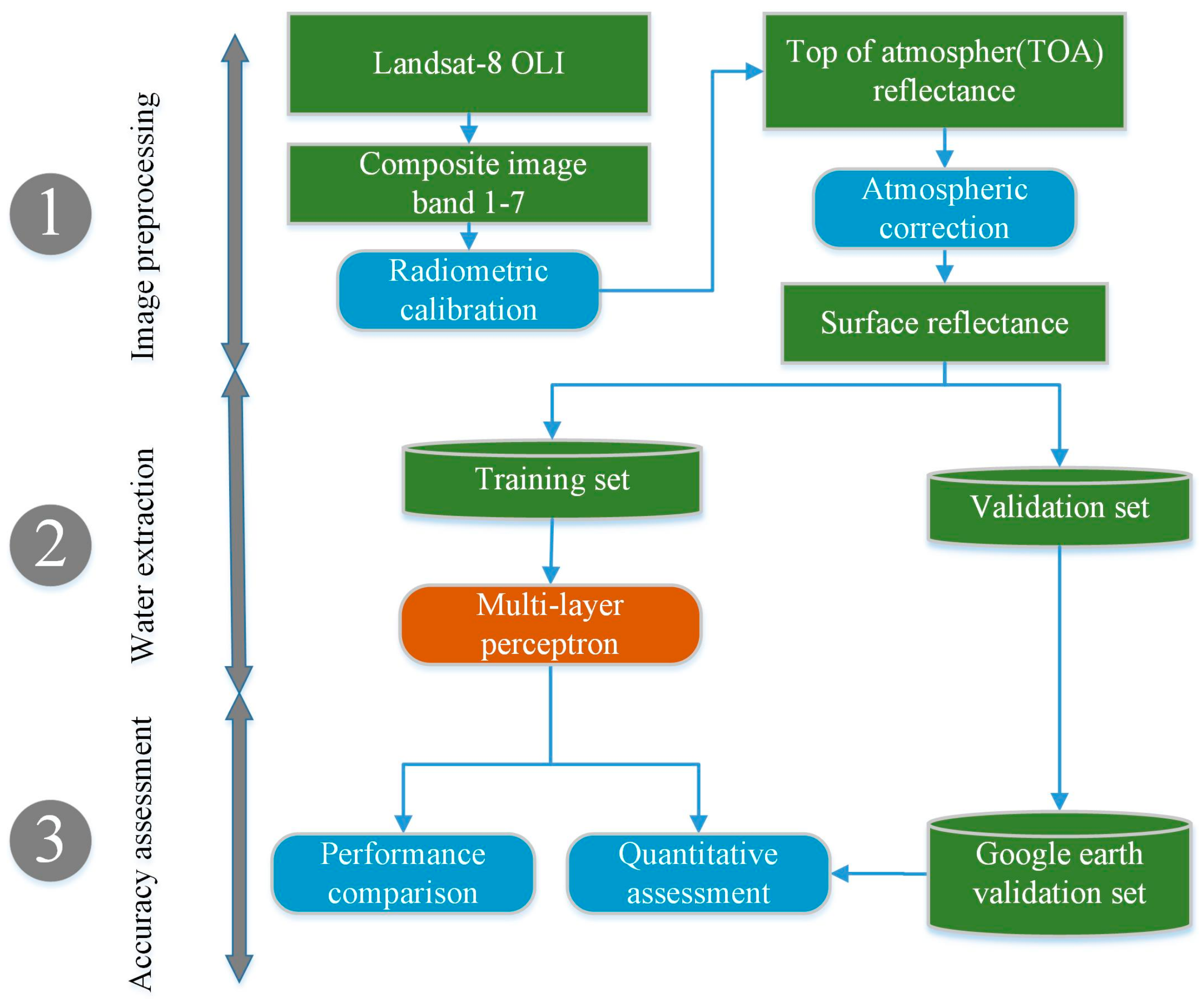
The flowchart of this study is shown in Figure 3. This flowchart contains three steps: image preprocessing, water extraction and an accuracy assessment. The first step generates surface reflectance from the Landsat 8 images by using radiometric calibration and atmospheric correction. Then, in the second step, to compare the performance of the MLP, the water index and support vector machine are also employed to extract surface water. The classification of the three classifiers for each study region are generated. Finally, random samples, which are validated with high-resolution Google Earth images, are collected to assess the classification accuracy. The performance of the MLP when extracting water types and suppressing noise is comprehensively compared with two other algorithms.
2.2.1. Image Preprocessing
To obtain a high-quality and consistent experimental dataset, the downloaded images should be radiometrically and atmospherically calibrated. Radiometric calibration can be divided into two steps. The first step calculates the top of atmosphere (TOA) radiances, RTOA, using the following equation [46]:
DN denotes the original digital number (DN) value. The variables a and b represent the gain factor and offset factor, respectively, which can be obtained from the metadata file.
The second step calculates the TOA reflectance, , which can correct errors in the Earth–Sun distance and the exo-atmospheric solar irradiance [47].
D represents the Earth-to-Sun distance; E0 denotes the mean exo-atmospheric solar irradiance; θ represents the solar zenith angle; and π = 3.1415926.
Furthermore, atmospheric correction is conducted using the 6S model (i.e., the second simulation of the satellite signal in the solar spectrum) with a digital elevation model (DEM) and atmospheric parameters (i.e., water vapor content, ozone and aerosol optical thickness), which are derived from MODIS atmospheric products [46]. Through the above preprocessing, the original data are converted into surface reflectance data.
2.2.2. Multilayer Perceptron
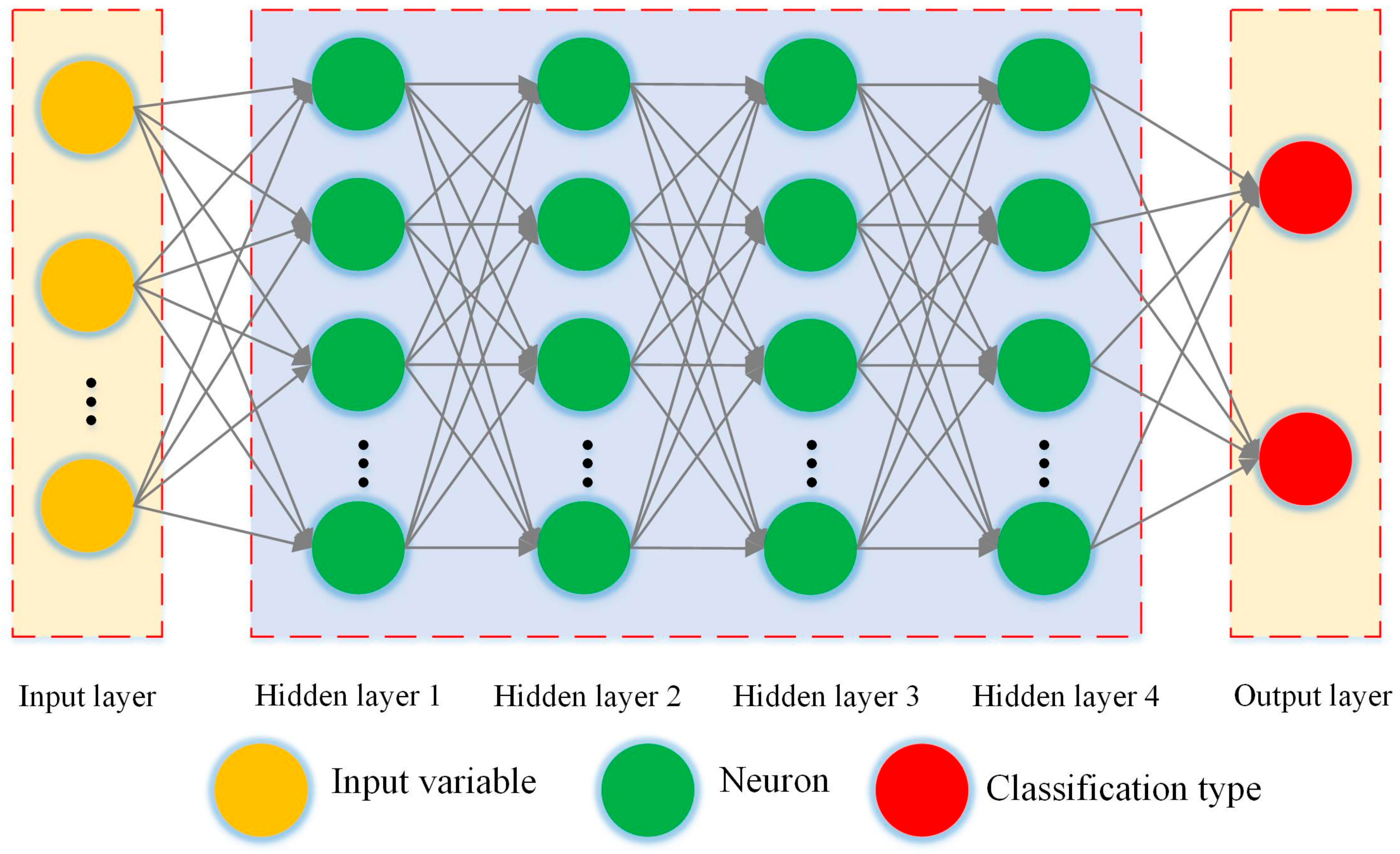
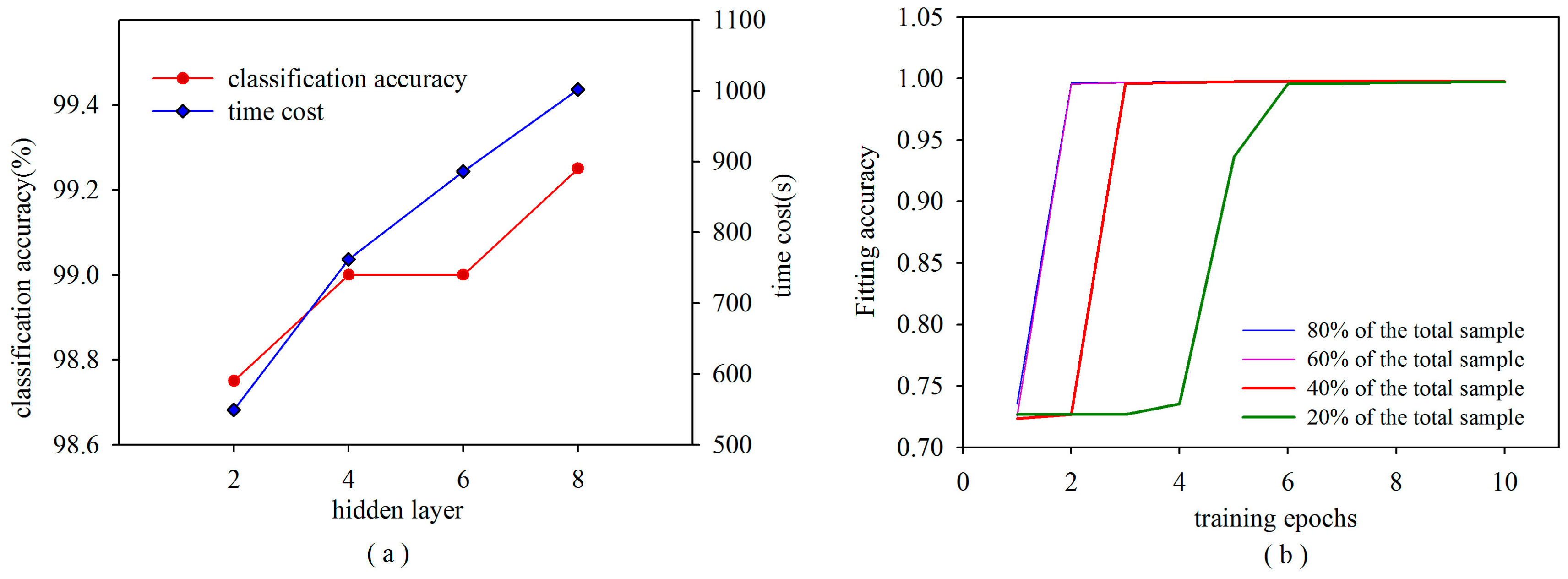
Multilayer perceptron is a neural network model with multiple hidden layers [48], and the neurons between adjacent layers are connected [44]. The architecture of the model is shown in Figure 4, and the parameters of the MLP are summarized in Table 2. The parameter selection involved in the proposed MLP is based on experience and experiment. As for the hidden layers’ selection, the comparison experiment is conducted by setting 2, 4, 6 and 8 hidden layers, and the result (Figure 5a) shows that with the layer increased, the time cost will sharply increase, while the accuracy will not be improved. When the layer is set as two, the classification accuracy is low. Therefore, to balance the accuracy and time cost [49,50], four hidden layers are selected in this experiment. The number of neurons for each hidden layer is set according to the experience of multiple trials, and the principle is still balancing time cost and accuracy. The activation function and loss function are ReLU and softmax cross-entropy with logits, respectively. The flow of the extraction contains three steps: sample selection, model training and classification generation.
- Sample selection: The training samples for each scene are manually labeled and cover all water types and non-water types. In this paper, all training samples are manually labeled in ENVI 5.3 using ROI for water and no-water. Each ROI consists of pixels within a polygon feature. The distribution of these samples is based on manual experience, and we try our best to improve representativeness and randomness of the spatial distribution. To ensure the accuracy of the sample, only identified non-water and water bodies will be selected as samples. The mixed pixels in coastal area, river banks and wetlands will not be considered. The sample numbers for all water and non-water types in each image are shown in Table 3. These samples are randomly divided into training samples and validation samples. According to the experiment, by setting different training sample percentages (Figure 5b), 80% of the total sample is used to train the model and to generate the fitting accuracy, and 20% of the total sample is used to verify the accuracy. To ensure the comparability of the algorithm accuracy, the training samples of the water and non-water bodies via the MLP and support vector machine are the same.
- Model training: Based on these training samples and the architecture, the surface reflectance variables of the seven bands in the labeled pixel are input into the model. During the forward propagation process, the activation function is used to compute the weights and biases with the labeled training samples. To optimize the weights and minimize the errors, a gradient descent algorithm is applied to train the network and identify the weights and biases of each layer during the back-propagation process.
- Classification generation: With the trained model, the probability of water and non-water types for each pixel are computed. The classification type depends on the probability value. Then, the classification results, which are labeled with different colors, can be generated.
TensorFlow [51], which is an open source platform developed by Google, is employed to implement the MLP with Python.
2.2.3. Accuracy Assessment
(1) Quantitative assessment:
To quantitatively evaluate the water extraction accuracy, the surface reflectance images of Landsat 8 are classified as various water and non-water types according to the categories of Table 3. Fifteen to 25 random points are generated for each layer using stratified random sampling, and the total validation points for water and non-water is 100, respectively. Then, these points are verified based on a high-resolution Google Earth image. The error matrix for the water classification for each scene is implemented with the validation points and classification results. Finally, based on the error matrix, the overall accuracy (OA) and kappa coefficients (KCs) can be calculated using the following equations [31]:
where N denotes the total number of pixels used in the accuracy assessment, represents the total number of correct pixels for the i-th class, represents the total number of i-th classes acquired from the classification result and represents the total number of i-th classes acquired from the validation data.
(2) Performance comparison:
To compare the performances of the proposed algorithms, two commonly-used methods (i.e., support vector machine [52] and water index [21]) are employed in this study. The radial basis function (RBF), which is an extensive function applied in the remote sensing classification field [53], is selected as the kernel function for the support vector machine. The SVM classification is implemented on the ENVI 5.3 platform, and the model parameters are summarized in Table 2. In addition, the value of gamma in the kernel function is set to 0.143 according the inverse of the number of bands.
Modification of the normalized difference water index (MNDWI) [21] is a widely-used water index that highlights water information [3,23]. In this study, the MNDWI, combined with the popular Otsu’s threshold segmentation method [18,54], is adopted to automatically extract surface water for a performance comparison.
3. Results
In this section, the performance of the surface water extraction for the entire scene is assessed first through visual comparisons and a quantitative index. Subsequently, detailed comparisons of the different water types are implemented to explore the universality of the proposed algorithm. Then, several noises are included to test the reliability of the proposed algorithm. Finally, the band optimization of the proposed algorithm is analyzed.
3.1. Classification Results and Accuracy Comparisons
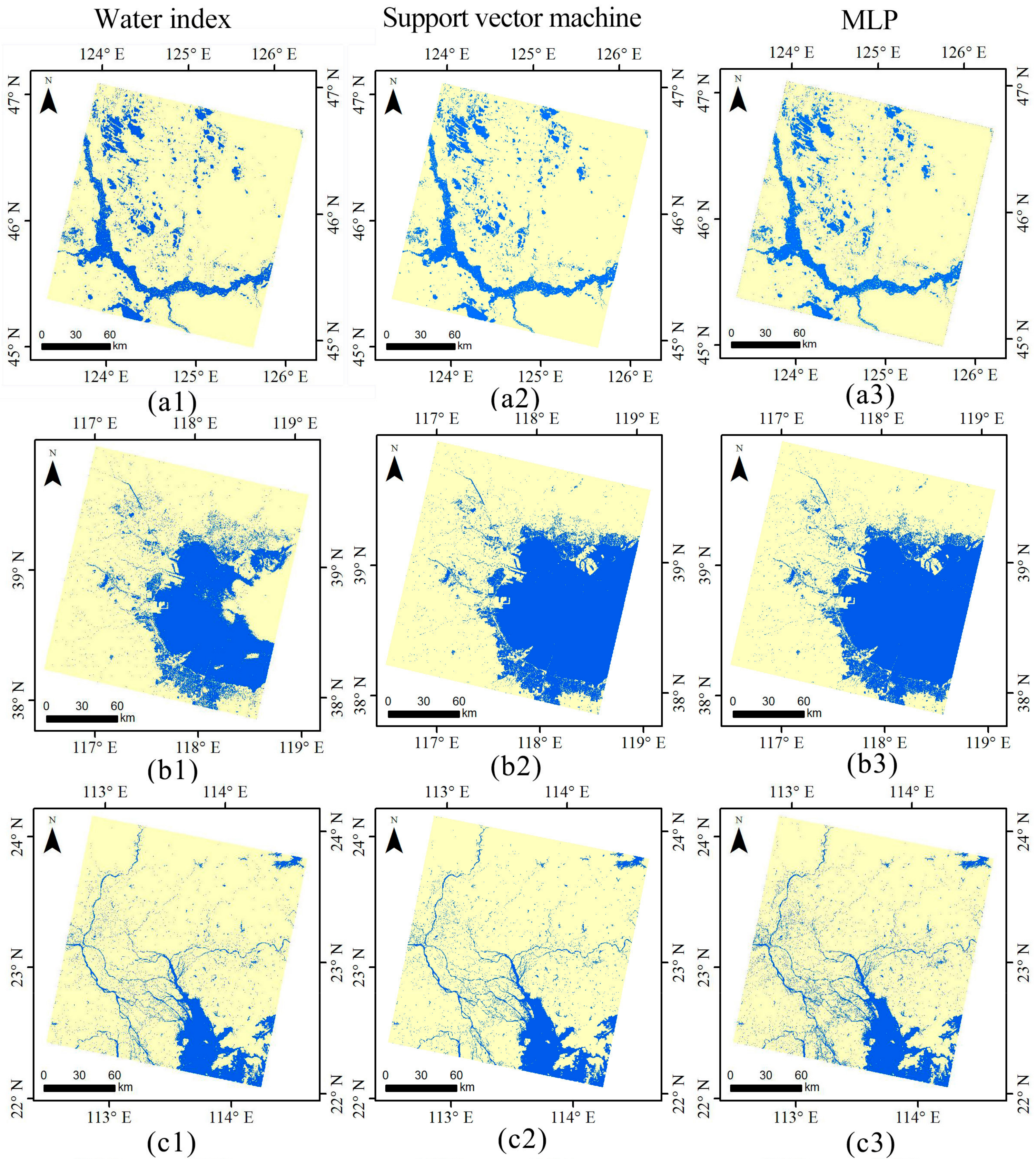
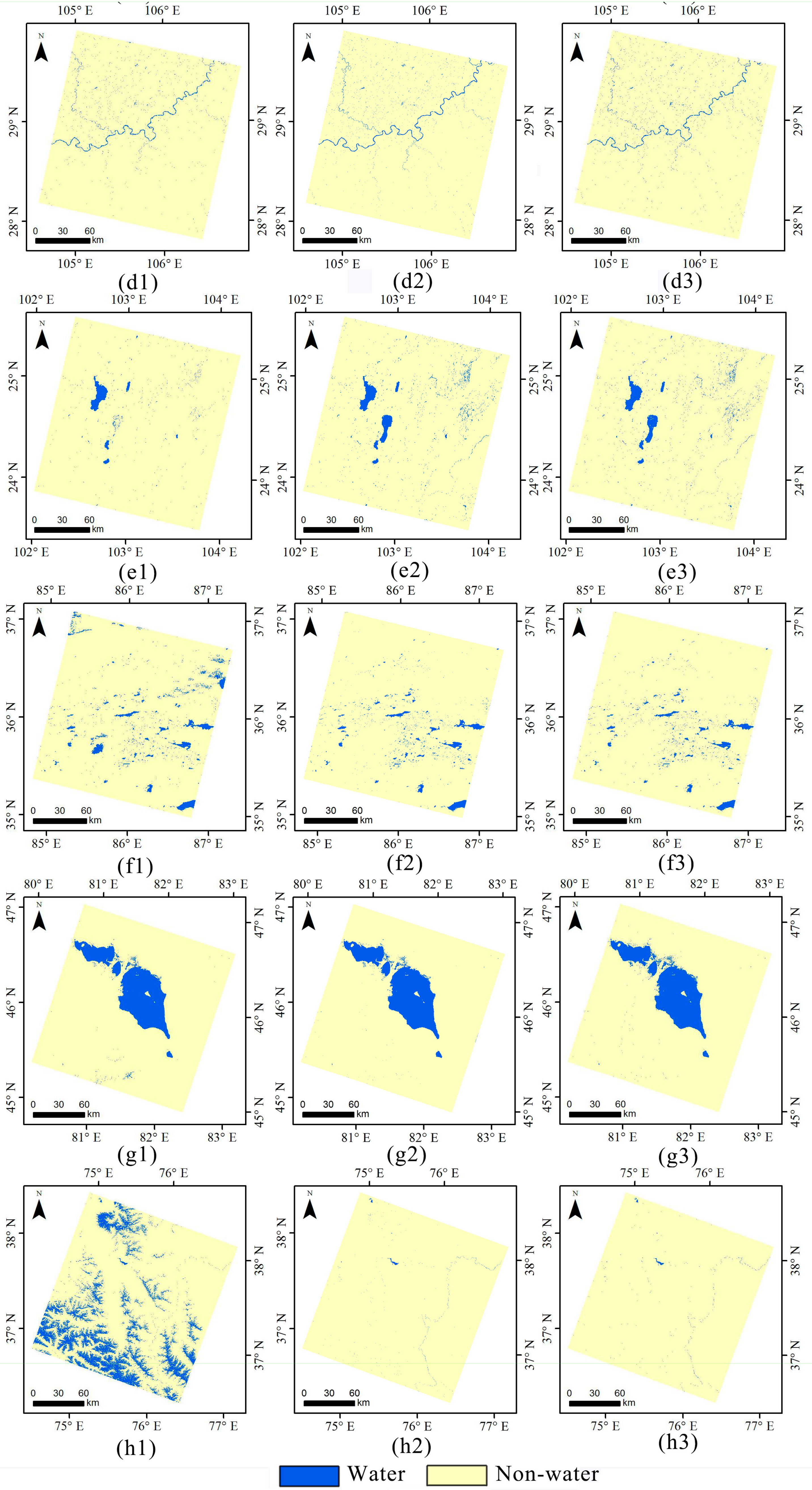
The classifications of the surface water extractions using the three algorithms in eight regions are shown in Figure 6. Based on the visual inspection, the patterns for surface water in Regions a and d are similar, while the performances in Regions b, c, e, f, g and h using the three classifiers are different. For Region b, some sea-water bodies are not extracted using the water index. Moreover, many detailed surface water bodies are not identified with the water index and the support vector machine in Region c and Region e. Generally, clouds, mountain shadows and ice/snow are obstacles when extracting surface water bodies. Compared with the classifications in Regions f, g and h, the MLP performs better than the water index, and the performances of the MLP and support vector machine are almost the same. Specifically, for Region h, the water index method cannot distinguish ice/snow from surface water bodies. Therefore, through visual comparison, the classification shows that the MLP can achieve an adequate performance for the entire image.
To quantitatively evaluate the accuracy of the surface water classification, the overall accuracy and kappa coefficients are calculated for each region, and the results are summarized in Table 4. When comparing the overall accuracy of the three methods in the eight study regions, the accuracy of the MLP is higher than those of the water index and the support vector machine. The overall accuracy of the MLP ranges from 98.25–100%; however, the overall accuracy of the water index ranges from 76.56–98.50%. The overall accuracy of the support vector machine is similar to that of the MLP, while the water index achieves the lowest accuracy of the three methods because Otsu’s threshold is highly dependent on the ratio between water and non-water surfaces [55]. The threshold of eight images ranges from 0.2157–0.4392. Furthermore, a comparison of the kappa coefficients shows that the kappa coefficients of the MLP are greater than those of the other two classifiers. The kappa coefficients of the water index in Regions e and h are still the lowest because this method misses several thin ponds and ice/snow noise. Based on this accuracy evaluation, the quantitative indices of MLP are greater than those of the water index and support vector machine. These results are consistent with the visual inspection.
3.2. Performance Comparison When Extracting Different Water Types
To assess the universality of the MLP algorithm, typical surface water bodies, including lakes, thin rivers, sea water, open ponds, turbid waters and aquacultural waters, are derived from the classification results in Section 3.1. A comparison is used to detect false water and true water bodies based the visual inspection and to analyze the reason for classification differences.
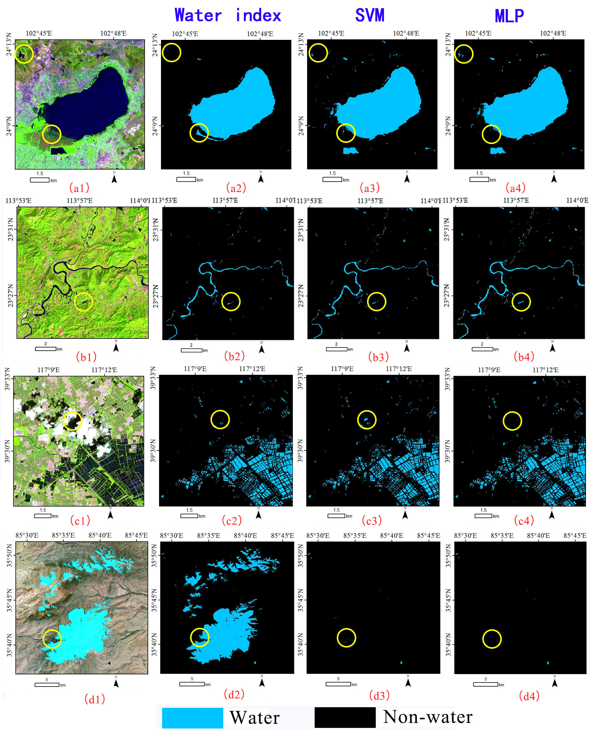
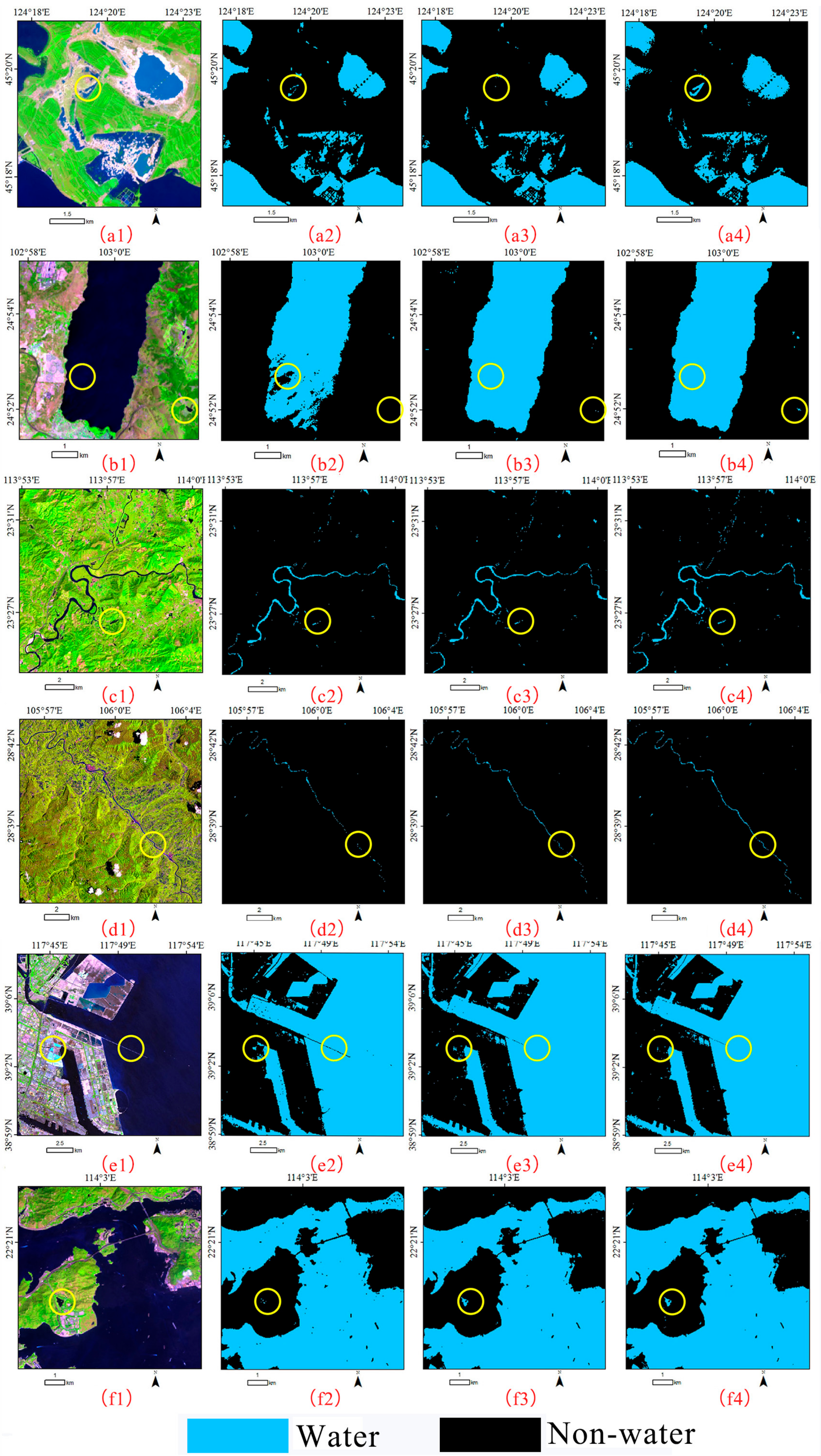
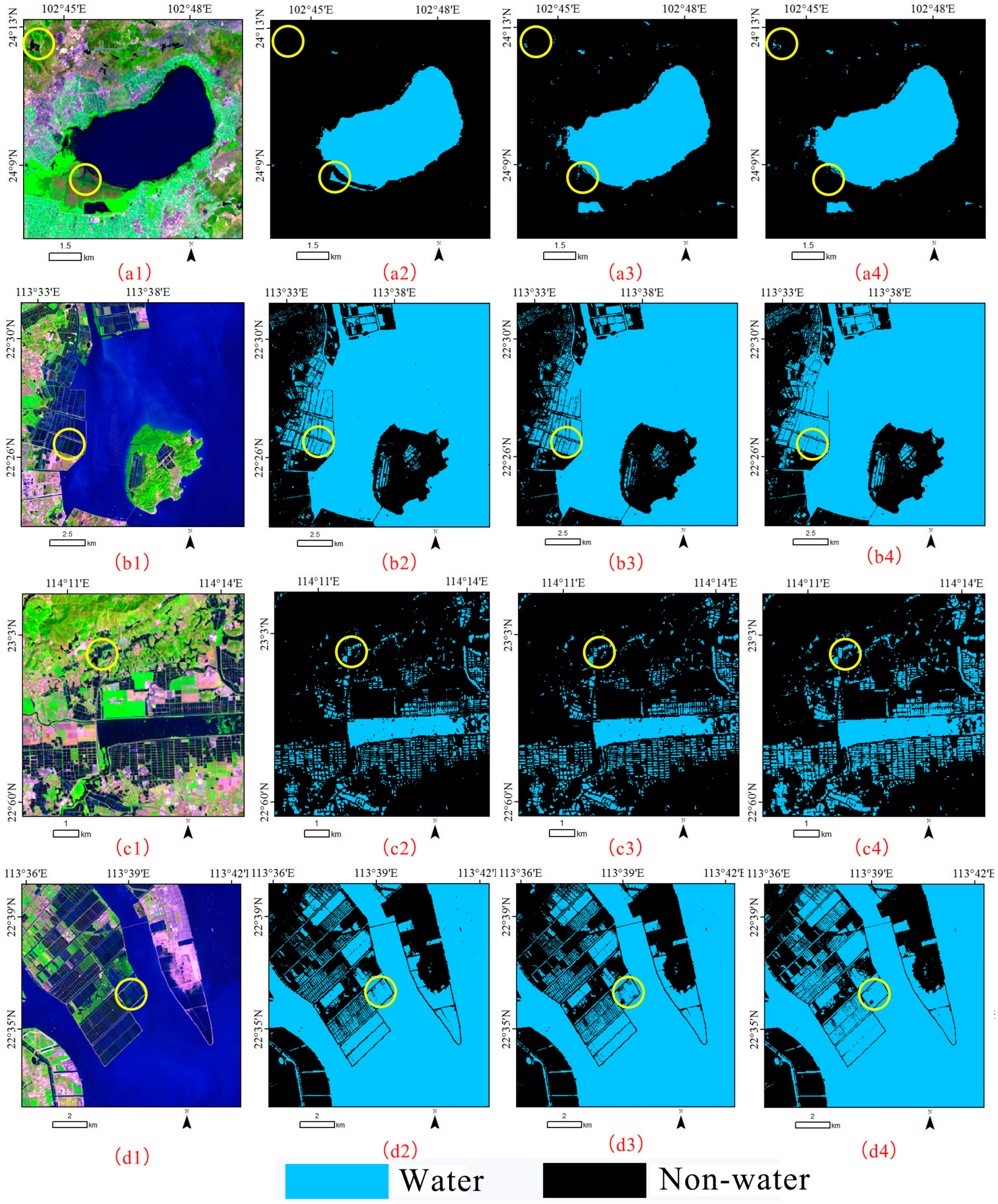
The performance comparison among lakes, thin rivers and sea water bodies is shown in Figure 7, and the differences in the extraction results are highlighted using a yellow circle. Regarding lakes, the local images, which are derived from Regions a and c, are shown in Figure 7(a1,b1), respectively. It can clearly be seen that the highlighted surface water in Figure 7(a3,b2) is missing, while the MLP method can exactly identify the surface water. This missing result may be related to the spectrum difference across the lake. Moreover, detailed thin rivers cannot be mapped with the support vector machine and water index, especially in Figure 7(c3,d2). For the extraction of sea water, the water index can distinguish land from sea water in Figure 7(e2), while it misses some water details in Figure 7(f2). The support vector machine can achieve almost the same performance as the MLP method when extracting sea water bodies.
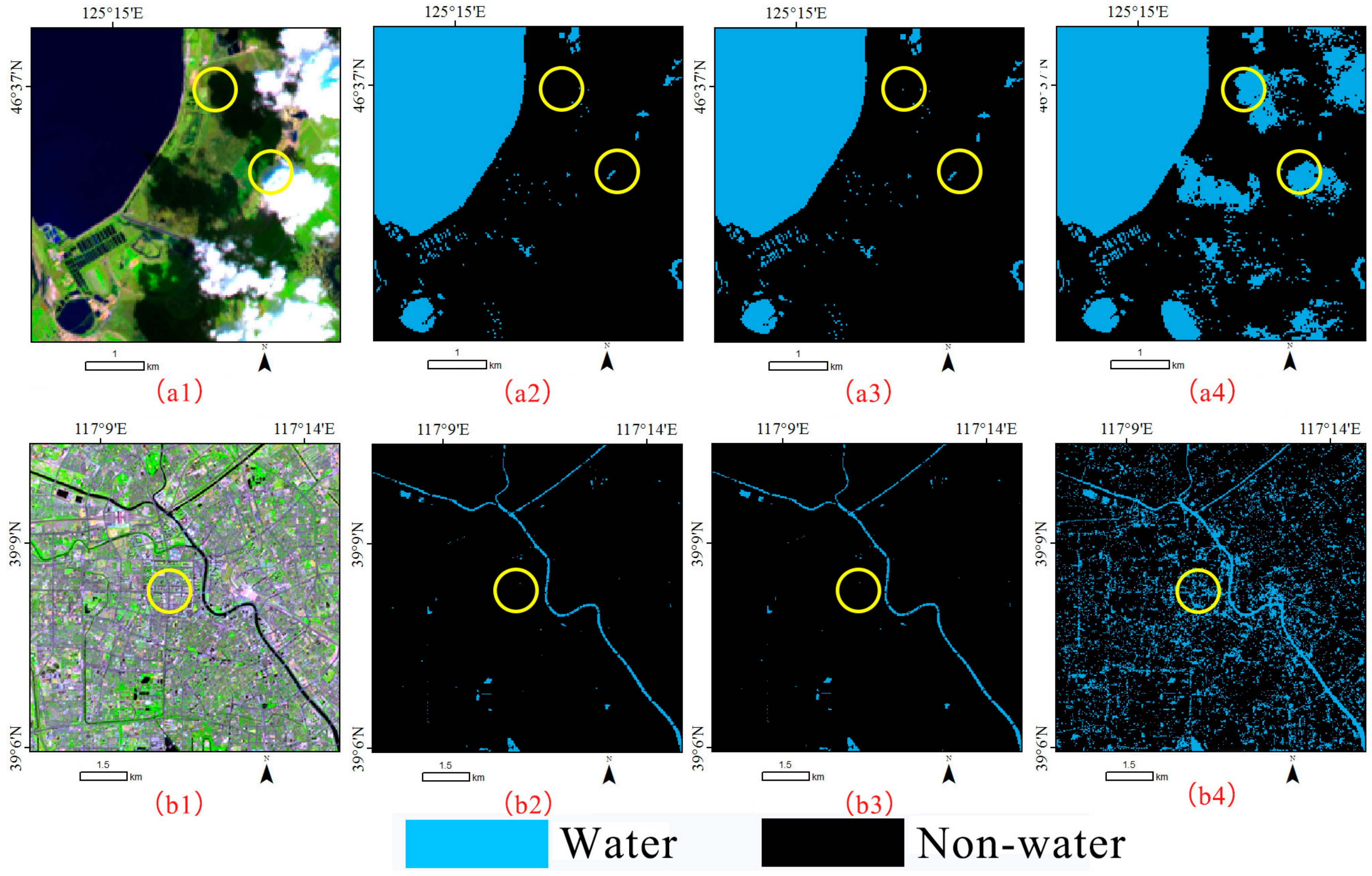
The performances of surface water mapping for open ponds, turbid waters and aquaculture areas are shown in Figure 8. For open ponds, the performance comparison shows that a large open pond can be precisely extracted with the three methods, while a smaller open pond is missed when using the water index and support vector machine. Moreover, mixing between surface water and wetlands causes a commission error in Figure 8(a2). The results of the turbid water area located in the Pearl River estuary and those demonstrating the performance of the surface water extraction are almost the same; however, the support vector machine misses several surface water bodies, as shown in Figure 8(b3). Two aquaculture areas (Figure 8(c1,d1)) are selected from Region c to compare the detailed surface water extractions. For these two areas, the surface water area using the MLP is larger than that using the other two algorithms, which demonstrates that the MLP performs better when identifying detailed surface water bodies, while several surface water bodies in Figure 8(c3,d3) using the support vector machine are missed. By analyzing Figure 7 and Figure 8, the MLP can achieve an adequate performance when extracting various surface water bodies, which confirms the universality of the proposed algorithm.
3.3. Performance Comparison When Suppressing Noise
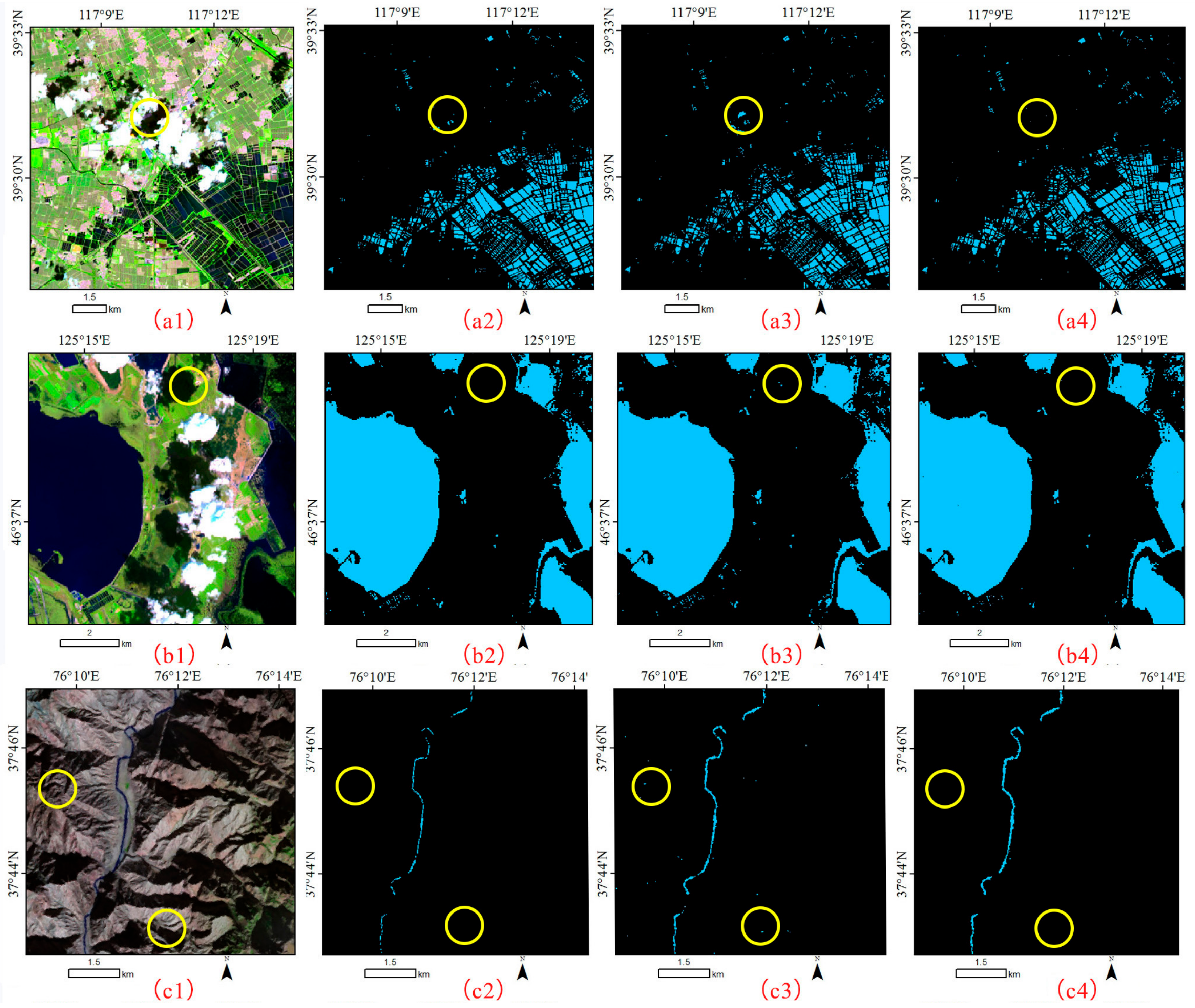
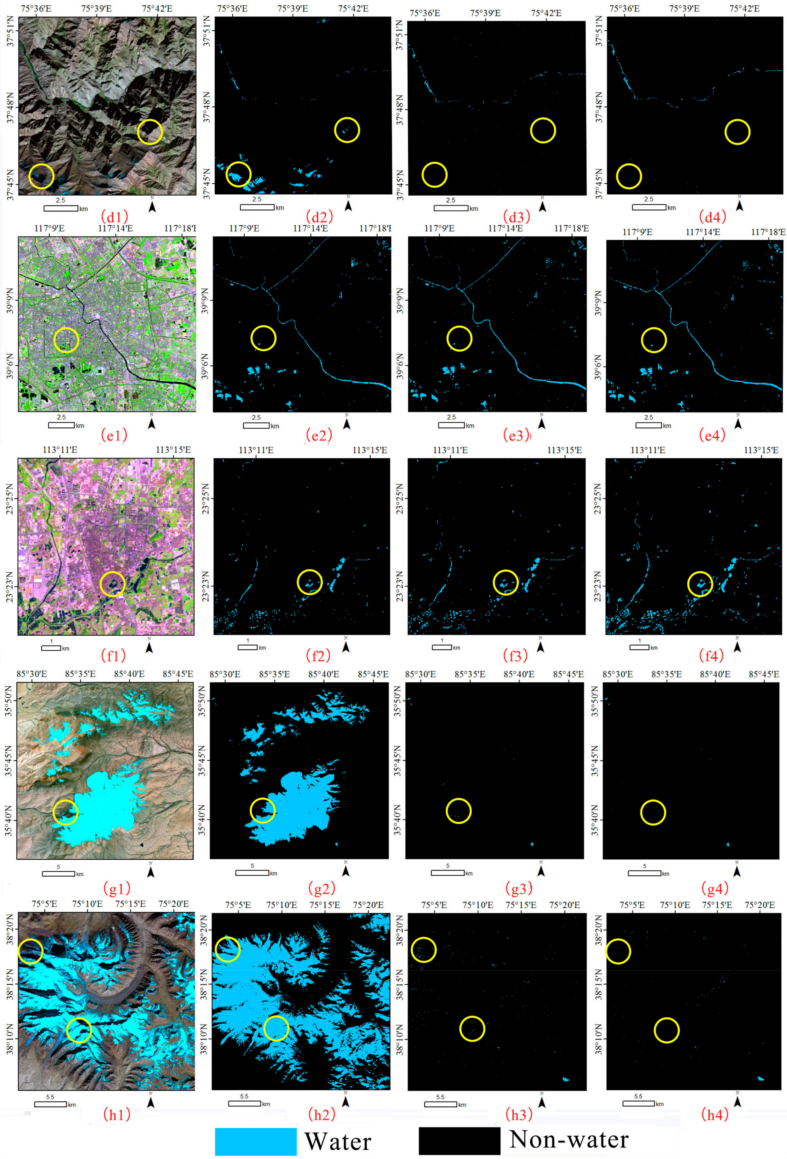
The spectrum for shadows and ice/snow is similar to that for surface water; thus, it is a challenge to remove these noises from surface water bodies in remote sensing images [9]. To examine the reliability of then MLP when suppressing noise, four major noise images, including cloud shadows, mountain shadows, building shadows and ice/snow, are derived from the studied dataset. Then, a performance comparison of these images is shown in Figure 9.
For cloud shadows, the surface water map results in Figure 9(a1,b1) show that cloud shadows can be removed using the water index and MLP methods; however, the support vector machine mixes some of the cloud shadows with the surface water. The performance of the MLP when suppressing mountain shadows is the best among the three methods (Figure 9(c1,d1)). The support vector machine can distinguish most of the mountain shadows in Figure 9(c3) and Figure 9(d3), but several shadows cannot be removed clearly in these regions. Figure 9e,f shows the experimental results for building shadows. The extraction map demonstrates that the performances when suppressing building noise are almost the same. Moreover, detailed surface water in urban areas can be precisely detected in Figure 9(f4). For the areas in Figure 9g,h, the water index algorithm causes serious mixing between ice/snow and surface water, and the extractions in Figure 9(g3,h3) still contain part of the mountain shadows, while the MLP can remove this noise.
For the performance comparison when suppressing noise, the water index cannot eliminate noise from ice/snow, mountain shadows and cloud shadows, and mountain shadows and ice/snow still exist in the classification map based on the support vector machine extraction. The three algorithms can efficiently suppress building shadows. Overall, the MLP achieves a better performance when suppressing noise compared to the other two algorithms.
3.4. Band Optimization for the Multilayer Perceptron Neural Network Method
Band optimization is necessary when using the MLP to extract surface water based on Landsat OLI images. Therefore, a band optimization experiment is conducted using the original band and several water indices, and the results are shown in Figure 10. There are significant errors in the cloud and cloud shadow detections in Figure 10(a4), and the building shadows in Figure 10(b4) are classified as surface water bodies; however, the performances in Figure 10(a2,a3,b2,b3) are very excellent. These results demonstrate that adding a water index cannot improve the accuracy of the surface water extraction, and the 1–7-band composite provides an adequate band optimization strategy for model training. This may be related to the multiple hidden layers of the MLP, which can fully train the image features [49].
4. Discussion
Deep learning is a hot topic in the era of artificial intelligence [34], and it has shown great promise in target identification and image classification from remote sensing images [61,62,63]. However, there is still a lack of studies regarding surface water extraction when using the MLP [29]. In this study, the classification accuracy of surface water in eight regions via a visual inspection and quantitative index is evaluated first. The results demonstrate that the classification accuracy of the MLP is higher than that of the other two methods. Subsequently, the performance of the MLP when extracting various surface water types is better than those of the water index and the support vector machine; moreover, the MLP can effectively suppress noise to improve the accuracy of surface water extraction.
Despite the fact that MLP achieves an adequate performance when mapping surface water, there are uncertainty factors that impact the mapping accuracies. The first one is image preprocessing. To ensure data consistency, a majority of surface water mapping is based on the top of atmosphere (TOA) reflectance or surface reflectance [3,9]. For surface water extraction based on single-scene images, there are almost no differences between the original image and the preprocessed image. However, for surface water mapping at a large scale, it is necessary to preprocess the image to improve the consistency of the proposed method.
The second factor is training samples. MLP belongs to a supervised classification; thus, the classification accuracy depends on the training samples. From a practical perspective when training the sample selections, all water and non-water bodies in the image should be selected, and the labeled training samples must be absolutely correct; otherwise, serious mixing between the water and non-water bodies occurs. To obtain high accuracies and various samples, manually-sampled selections are employed in this study. However, this limits the automation of the proposed algorithm. Fortunately, given several high-resolution surface water products that have been released during recent years [9,16], the automation of the proposed algorithm is further improved by using these reference products to generate high-quality training samples.
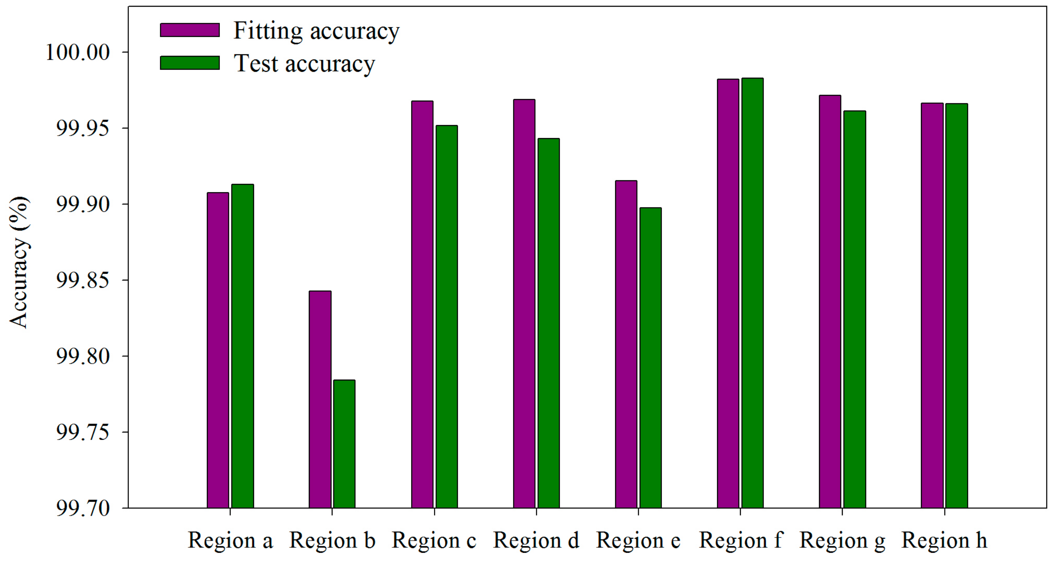
To further illustrate the reliability of the proposed method, the model accuracies for each study region are shown in Figure 11. The figure shows that the fitted accuracy and the tested accuracy are greater than 99.75%, which demonstrates the advantage of an MLP classifier when extracting surface water. This result may explain why the MLP achieves higher accuracies compared to support vector machine extraction with the same training samples. Another advantage of the MLP is a model without a threshold, which may be suitable for the extraction of surface water with multiple scenarios and multiple satellite images. Moreover, if there is a large number of samples to train and optimize the algorithm, the universality of the proposed algorithm is further improved, which can be used when mapping surface water at a global scale. In addition, this method can not only be used to identify surface water, but it also has the potential to extract other types of land cover, such as urban areas, farmlands and forests [29].
5. Conclusions
Deep learning shows great promise for target identification and image classification. This study employs an MLP neural network to extract surface water bodies in Landsat 8 OLI images. Eight images of typical regions are selected, and two other algorithms (i.e., the water index and the support vector machine) are included to compare their performances when extracting surface water. Then, the performances of various surface water extractions and noise suppressions are comprehensively compared. Finally, band optimization and uncertainty factors that impact the accuracy of the surface water extraction when using the MLP neural network are summarized. The conclusions are summarized as follows:
- (1)
- Based on a visual comparison, the performance of the MLP when extracting surface water is better than those with the water index and support vector machine. Moreover, a quantitative evaluation shows that the overall accuracy and kappa coefficients of the MLP are higher than those of the other two classifiers. The overall accuracy of the MLP ranges from 98.25–100%, and the kappa coefficients of the MLP range from 0.965–1.
- (2)
- Compared with the water index and the support vector machine, the performance of the MLP demonstrates that it can precisely extract six types of surface water bodies (i.e., lakes, thin rivers, sea water, open ponds, turbid waters and aquacultural water), and detailed surface water can be identified. Furthermore, the MLP can effectively suppress noise when extracting surface water, such as cloud shadows, mountain shadows, building shadows and ice/snow.
- (3)
- For the MLP algorithm, the 1–7-band composite is a better band optimization strategy, and image preprocessing and high-quality samples can reduce the uncertainty of the extraction. Based on newly-released surface water products, automation of the proposed algorithm will be improved. Moreover, the algorithm is also suitable for Landsat series images or other high-resolution images when identifying surface water.
This study introduces an MLP neural network for the extraction of surface water, and the results confirm that this proposed method can achieve an adequate performance. For future studies, the automation and universality of the proposed algorithm can be further enhanced using newly-released surface water products. Then, the proposed method can be used to map global surface water, which can help us understand the changes in surface water patterns under a background of global change.
Author Contributions
G.H., W.J. and T.L. conceived of and designed the experiments. W.J. and Y.N. performed the experiments. W.J. and T.L. analyzed the data. H.L., K.L., Y.P. and G.W. provided assistance in preparing the related graphs. W.J. wrote the whole paper, and all authors edited the paper. The authors thank the three anonymous reviewers and the editors for their valuable comments to improve our manuscript.
Acknowledgments
This research was financially supported by the National Key Research and Development Program of China (2016YFA0600302), the Strategic Priority Research Program of the Chinese Academy of Sciences(XDA190090300), the National Natural Science Foundation of China (61731022 and 61701495) and the Hainan Provincial Department of Science and Technology (Grant Numbers ZDKJ2016021 and ZDKJ2016015).
Conflicts of Interest
The authors declare no conflicts of interest.
References
- Oki, T.; Kanae, S. Global hydrological cycles and world water resources. Science 2006, 313, 1068–1072. [Google Scholar] [CrossRef] [PubMed]
- Haddeland, I.; Heinke, J.; Biemans, H.; Eisner, S.; Florke, M.; Hanasaki, N.; Konzmann, M.; Ludwig, F.; Masaki, Y.; Schewe, J.; et al. Global water resources affected by human interventions and climate change. Proc. Natl. Acad. Sci. USA 2014, 111, 3251–3256. [Google Scholar] [CrossRef] [PubMed]
- Feng, M.; Sexton, J.O.; Channan, S.; Townshend, J.R. A global, high-resolution (30-m) inland water body dataset for 2000: First results of a topographic-spectral classification algorithm. Int. J. Digit. Earth 2016, 9, 113–133. [Google Scholar] [CrossRef]
- Mekonnen, M.M.; Hoekstra, A.Y. Four billion people facing severe water scarcity. Sci. Adv. 2016, 2, e1500323. [Google Scholar] [CrossRef] [PubMed]
- Hirabayashi, Y.; Mahendran, R.; Koirala, S.; Konoshima, L.; Yamazaki, D.; Watanabe, S.; Kim, H.; Kanae, S. Global flood risk under climate change. Nat. Clim. Chang. 2013, 3, 816–821. [Google Scholar] [CrossRef]
- Pahl-Wostl, C. Transitions towards adaptive management of water facing climate and global change. Water Resour. Manag. 2007, 21, 49–62. [Google Scholar] [CrossRef]
- Vorosmarty, C.J.; McIntyre, P.B.; Gessner, M.O.; Dudgeon, D.; Prusevich, A.; Green, P.; Glidden, S.; Bunn, S.E.; Sullivan, C.A.; Liermann, C.R.; et al. Global threats to human water security and river biodiversity. Nature 2010, 467, 555–561. [Google Scholar] [CrossRef] [PubMed]
- Chini, M.; Hostache, R.; Giustarini, L.; Matgen, P. A hierarchical split-based approach for parametric thresholding of SAR images: Flood inundation as a test case. IEEE Geosci. Remote Sens. 2017, 55, 6975–6988. [Google Scholar] [CrossRef]
- Yamazaki, D.; Trigg, M.A.; Ikeshima, D. Development of a global similar to 90 m water body map using multi-temporal landsat images. Remote Sens. Environ. 2015, 171, 337–351. [Google Scholar] [CrossRef] [Green Version]
- Milly, P.C.D.; Dunne, K.A.; Vecchia, A.V. Global pattern of trends in streamflow and water availability in a changing climate. Nature 2005, 438, 347–350. [Google Scholar] [CrossRef] [PubMed]
- Carroll, M.L.; Townshend, J.R.; DiMiceli, C.M.; Noojipady, P.; Sohlberg, R.A. A new global raster water mask at 250 m resolution. Int. J. Digit. Earth 2009, 2, 291–308. [Google Scholar] [CrossRef]
- Valentini, N.; Saponieri, A.; Molfetta, M.G.; Damiani, L. New algorithms for shoreline monitoring from coastal video systems. Earth Sci. Inform. 2017, 10, 495–506. [Google Scholar] [CrossRef]
- Bruno, M.F.; Molfetta, M.G.; Mossa, M.; Nutricato, R.; Morea, A.; Chiaradia, M.T. Coastal observation through COSMO-skymed high-resolution SAR images. J. Coast. Res. 2016, 75, 795–799. [Google Scholar] [CrossRef]
- Ji, L.Y.; Gong, P.; Geng, X.R.; Zhao, Y.C. Improving the accuracy of the water surface cover type in the 30 m from-glc product. Remote Sens. 2015, 7, 13507–13527. [Google Scholar] [CrossRef]
- Liao, A.P.; Chen, L.J.; Chen, J.; He, C.Y.; Cao, X.; Chen, J.; Peng, S.; Sun, F.D.; Gong, P. High-resolution remote sensing mapping of global land water. Sci. China-Earth Sci. 2014, 57, 2305–2316. [Google Scholar] [CrossRef]
- Pekel, J.F.; Cottam, A.; Gorelick, N.; Belward, A.S. High-resolution mapping of global surface water and its long-term changes. Nature 2016, 540, 418–422. [Google Scholar] [CrossRef] [PubMed]
- Frazier, P.S.; Page, K.J. Water body detection and delineation with Landsat tm data. Photogram. Eng. Remote Sens. 2000, 66, 1461–1467. [Google Scholar]
- Xie, H.; Luo, X.; Xu, X.; Pan, H.Y.; Tong, X.H. Evaluation of Landsat 8 OLI imagery for unsupervised inland water extraction. Int. J. Remote Sens. 2016, 37, 1826–1844. [Google Scholar] [CrossRef]
- Du, Y.; Zhang, Y.H.; Ling, F.; Wang, Q.M.; Li, W.B.; Li, X.D. Water bodies' mapping from sentinel-2 imagery with modified normalized difference water index at 10-m spatial resolution produced by sharpening the SWIR band. Remote Sens. 2016, 8, 354. [Google Scholar] [CrossRef] [Green Version]
- McFeeters, S.K. The use of the normalized difference water index (NDWI) in the delineation of open water features. Int. J. Remote Sens. 1996, 17, 1425–1432. [Google Scholar] [CrossRef]
- Xu, H.Q. Modification of normalised difference water index (NDWI) to enhance open water features in remotely sensed imagery. Int. J. Remote Sens. 2006, 27, 3025–3033. [Google Scholar] [CrossRef]
- Feyisa, G.L.; Meilby, H.; Fensholt, R.; Proud, S.R. Automated water extraction index: A new technique for surface water mapping using landsat imagery. Remote Sens. Environ. 2014, 140, 23–35. [Google Scholar] [CrossRef]
- Zhou, Y.; Dong, J.W.; Xiao, X.M.; Xiao, T.; Yang, Z.Q.; Zhao, G.S.; Zou, Z.H.; Qin, Y.W. Open surface water mapping algorithms: A comparison of water-related spectral indices and sensors. Water 2017, 9, 16. [Google Scholar] [CrossRef]
- Huang, X.; Xie, C.; Fang, X.; Zhang, L.P. Combining pixel- and object-based machine learning for identification of water-body types from urban high-resolution remote-sensing imagery. IEEE J. Sel. Top. Appl. Earth Obs. Remote Sens. 2015, 8, 2097–2110. [Google Scholar] [CrossRef]
- Yang, F.; Guo, J.H.; Tan, H.; Wang, J.X. Automated extraction of urban water bodies from zy-3 multi-spectral imagery. Water 2017, 9, 27. [Google Scholar] [CrossRef]
- Shao, P.; Yang, G.D.; Niu, X.F.; Zhang, X.Q.; Zhan, F.L.; Tang, T.Q. Information extraction of high-resolution remotely sensed image based on multiresolution segmentation. Sustainability 2014, 6, 5300–5310. [Google Scholar] [CrossRef]
- Zhao, P.X.; Zhao, J.; Wu, J.H.; Yang, Y.Z.; Xue, W.; Hou, Y.C. Integration of multi-classifiers in object-based methods for forest classification in the loess plateau, china. Scienceasia 2016, 42, 283–289. [Google Scholar] [CrossRef]
- Vanderhoof, M.K.; Distler, H.E.; Mendiola, D.T.G.; Lang, M. Integrating radarsat-2, lidar, and worldview-3 imagery to maximize detection of forested inundation extent in the delmarva peninsula, USA. Remote Sens. 2017, 9, 25. [Google Scholar] [CrossRef]
- Isikdogan, F.; Bovik, A.C.; Passalacqua, P. Surface water mapping by deep learning. IEEE J. Sel. Top. Appl. Earth Obs. Remote Sens. 2017, 10, 4909–4918. [Google Scholar] [CrossRef]
- Yao, F.F.; Wang, C.; Dong, D.; Luo, J.C.; Shen, Z.F.; Yang, K.H. High-resolution mapping of urban surface water using zy-3 multi-spectral imagery. Remote Sens. 2015, 7, 12336–12355. [Google Scholar] [CrossRef]
- Acharya, T.D.; Lee, D.H.; Yang, I.T.; Lee, J.K. Identification of water bodies in a Landsat 8 OLI image using a j48 decision tree. Sensors 2016, 16, 1075. [Google Scholar] [CrossRef] [PubMed]
- Rokni, K.; Ahmad, A.; Solaimani, K.; Hazini, S. A new approach for surface water change detection: Integration of pixel level image fusion and image classification techniques. Int. J. Appl. Earth Obs. Geoinf. 2015, 34, 226–234. [Google Scholar] [CrossRef]
- Ji, L.Y.; Geng, X.R.; Sun, K.; Zhao, Y.C.; Gong, P. Target detection method for water mapping using Landsat 8 OLI/TIRS imagery. Water 2015, 7, 794–817. [Google Scholar] [CrossRef]
- Guo, Y.M.; Liu, Y.; Oerlemans, A.; Lao, S.Y.; Wu, S.; Lew, M.S. Deep learning for visual understanding: A review. Neurocomputing 2016, 187, 27–48. [Google Scholar] [CrossRef]
- Zhang, L.P.; Zhang, L.F.; Du, B. Deep learning for remote sensing data a technical tutorial on the state of the art. IEEE Geosci. Remote Sens. Mag. 2016, 4, 22–40. [Google Scholar] [CrossRef]
- Taravat, A.; Proud, S.; Peronaci, S.; Del Frate, F.; Oppelt, N. Multilayer perceptron neural networks model for meteosat second generation SEVIRI daytime cloud masking. Remote Sens. 2015, 7, 1529–1539. [Google Scholar] [CrossRef] [Green Version]
- Li, W.J.; Fu, H.H.; Yu, L.; Cracknell, A. Deep learning based oil palm tree detection and counting for high-resolution remote sensing images. Remote Sens. 2017, 9, 13. [Google Scholar] [CrossRef]
- Albert, A.; Kaur, J.; Gonzalez, M.C. Using convolutional networks and satellite imagery to identify patterns in urban environments at a large scale. In Proceedings of the 23rd ACM SIGKDD International Conference on Knowledge Discovery and Data Mining, Halifax, NS, Canada, 13–17 August 2017. [Google Scholar]
- Yu, X.R.; Wu, X.M.; Luo, C.B.; Ren, P. Deep learning in remote sensing scene classification: A data augmentation enhanced convolutional neural network framework. GISci. Remote Sens. 2017, 54, 741–758. [Google Scholar] [CrossRef]
- Kussul, N.; Lavreniuk, M.; Skakun, S.; Shelestov, A. Deep learning classification of land cover and crop types using remote sensing data. IEEE Geosci. Remote Sens. Lett. 2017, 14, 778–782. [Google Scholar] [CrossRef]
- Zhao, W.Z.; Guo, Z.; Yue, J.; Zhang, X.Y.; Luo, L.Q. On combining multiscale deep learning features for the classification of hyperspectral remote sensing imagery. Int. J. Remote Sens. 2015, 36, 3368–3379. [Google Scholar] [CrossRef]
- Yu, L.; Wang, Z.; Tian, S.; Ye, F.; Ding, J.; Kong, J. Convolutional neural networks for water body extraction from Landsat imagery. Int. J. Comput. Intell. Appl. 2017, 16, 1750001. [Google Scholar] [CrossRef]
- Thakur, A.; Mishra, D. Hyper Spectral Image Classification Using Multilayer Perceptron Neural Network & Functional Link Ann; IEEE: New York, NY, USA, 2017; pp. 639–642. [Google Scholar]
- Patra, S.; Ghosh, S.; Ghosh, A. Change detection of remote sensing images with semi-supervised multilayer perceptron. Fundam. Inform. 2008, 84, 429–442. [Google Scholar]
- USGS Global Visualization Viewer (GloVis). Available online: https://glovis.usgs.gov/ (accessed on 2 December 2017).
- Peng, Y.; He, G.J.; Zhang, Z.M.; Long, T.F.; Wang, M.M.; Ling, S.G. Study on atmospheric correction approach of landsat-8 imageries based on 6s model and look-up table. J. Appl. Remote Sens. 2016, 10, 045006. [Google Scholar] [CrossRef]
- Yang, Y.H.; Liu, Y.X.; Zhou, M.X.; Zhang, S.Y.; Zhan, W.F.; Sun, C.; Duan, Y.W. Landsat 8 OLI image based terrestrial water extraction from heterogeneous backgrounds using a reflectance homogenization approach. Remote Sens. Environ. 2015, 171, 14–32. [Google Scholar] [CrossRef]
- Atkinson, P.M.; Tatnall, A.R.L. Neural networks in remote sensing–introduction. Int. J. Remote Sens. 1997, 18, 699–709. [Google Scholar] [CrossRef]
- Iliadis, M.; Spinoulas, L.; Katsaggelos, A.K. Deep fully-connected networks for video compressive sensing. Digit. Signal Prog. 2018, 72, 9–18. [Google Scholar] [CrossRef]
- Madhiarasan, M.; Deepa, S.N. Comparative analysis on hidden neurons estimation in multi layer perceptron neural networks for wind speed forecasting. Artif. Intell. Rev. 2017, 48, 449–471. [Google Scholar] [CrossRef]
- Tensorflow. Available online: https://www.tensorflow.org/ (accessed on 2 March 2018).
- Maulik, U.; Chakraborty, D. Remote sensing image classification a survey of support-vector-machine-based advanced techniques. IEEE Geosci. Remote Sens. Mag. 2017, 5, 33–52. [Google Scholar] [CrossRef]
- Cao, X.; Chen, J.; Matsushita, B.; Imura, H.; Wang, L. An automatic method for burn scar mapping using support vector machines. Int. J. Remote Sens. 2009, 30, 577–594. [Google Scholar] [CrossRef]
- Fisher, A.; Flood, N.; Danaher, T. Comparing Landsat water index methods for automated water classification in eastern Australia. Remote Sens. Environ. 2016, 175, 167–182. [Google Scholar] [CrossRef]
- Zhai, K.; Wu, X.; Qin, Y.; Du, P. Comparison of surface water extraction performances of different classic water indices using OLI and TM imageries in different situations. Geo-Spat. Inf. Sci. 2015, 18, 32–42. [Google Scholar] [CrossRef]
- Lu, S.L.; Wu, B.F.; Yan, N.N.; Wang, H. Water body mapping method with hj-1a/b satellite imagery. Int. J. Appl. Earth Obs. Geoinf. 2011, 13, 428–434. [Google Scholar] [CrossRef]
- Lacaux, J.P.; Tourre, Y.M.; Vignolles, C.; Ndione, J.A.; Lafaye, M. Classification of ponds from high-spatial resolution remote sensing: Application to rift valley fever epidemics in Senegal. Remote Sens. Environ. 2007, 106, 66–74. [Google Scholar] [CrossRef]
- Rogers, A.S.; Kearney, M.S. Reducing signature variability in unmixing coastal marsh thematic mapper scenes using spectral indices. Int. J. Remote Sens. 2004, 25, 2317–2335. [Google Scholar] [CrossRef]
- Xiao, Y.; Zhao, W.; Zhu, L. A study on information extraction of water body using band1 and band7 of tm imagery. Sci. Surv. Map. 2010, 35, 226–227. [Google Scholar]
- Shen, L.; Li, C.C. Water body extraction from Landsat ETM+ imagery using adaboost algorithm. In Proceedings of the 2010 18th International Conference on Geoinformatics, Beijing, China, 18–20 June 2010; Volume 4. [Google Scholar]
- Zhang, L.P.; Xia, G.S.; Wu, T.F.; Lin, L.; Tai, X.C. Deep learning for remote sensing image understanding. J. Sens. 2016, 2016, 7954154. [Google Scholar] [CrossRef]
- Zou, Q.; Ni, L.H.; Zhang, T.; Wang, Q. Deep learning based feature selection for remote sensing scene classification. IEEE Geosci. Remote Sens. Lett. 2015, 12, 2321–2325. [Google Scholar] [CrossRef]
- Das, M.; Ghosh, S.K. Deep-step: A deep learning approach for spatiotemporal prediction of remote sensing data. IEEE Geosci. Remote Sens. Lett. 2016, 13, 1984–1988. [Google Scholar] [CrossRef]
Figure 1.
The locations of the study regions.

Figure 2.
Eight images of the typical regions used in this study ((a–h) are the Landsat OLI band composite (R: Band 6; G: Band 5; B: Band 4) images of eight study areas).
Figure 2.
Eight images of the typical regions used in this study ((a–h) are the Landsat OLI band composite (R: Band 6; G: Band 5; B: Band 4) images of eight study areas).

Figure 3.
Overall flowchart adopted in this study.

Figure 4.
The architecture of the MLP used in this paper.

Figure 5.
The experiments of the MLP parameter. (a) Classification accuracy and time cost by setting different hidden layers and (b) fitting accuracy by setting different percentages of the training sample. To highlight the differences in the four experiments, the top ten training epochs are selected.

Figure 6.
The classification comparison of the three algorithms in eight study regions ((a1–h1) are the water index classification results; (a2–h2) are the support vector machine classification results; and (a3–h3) are the MLP classification results).
Figure 6.
The classification comparison of the three algorithms in eight study regions ((a1–h1) are the water index classification results; (a2–h2) are the support vector machine classification results; and (a3–h3) are the MLP classification results).


Figure 7.
The performance comparison for lakes (a1,b1), thin rivers (c1,d1) and sea water bodies (e1,f1). (a2–h2) are the water index classification results; (a3–h3) are the support vector machine classification results; and (a4–h4) are the MLP classification results. Yellow circle are used to highlight the differences of three extraction results.

Figure 8.
The performance comparison for open ponds (a1), turbid waters (b1) and aquacultural waters (c1,d1). (a2–d2) are the water index classification results; (a3–d3) are the support vector machine classification results; and (a4–d4) are the MLP classification results. Yellow circle are used to highlight the differences of three extraction results.

Figure 9.
The performance comparison when suppressing noise from cloud shadows (a1,b1), mountain shadows (c1,d1), building shadows (e1,f1) and ice/snow (g1,h1). (a2–h2) are the water index classification results; (a3–h3) are the support vector machine classification results; and (a4–h4) are the MLP classification results. Yellow circle are used to highlight the differences of three extraction results.


Figure 10.
Performance comparisons based on band selection. (a1,b1) are the original images; (a2,b2) are the classification results only based on the 1–7-band composite; (a3,b3) are the classification results based on the composite of Bands 1–7, the NDWI1 [20], MNDWI [21] and NDVI [56]; (a4,b4) are the classification results based on the composite of eight water indices, including the NDWI1 [20], MNDWI [21], NDVI [56], NDPI [57], NDWI3 [58], NEW [59] and WRI [60]. Yellow circle are used to highlight the differences of three extraction results.

Figure 11.
The accuracy of the MLP for each study region.


Table 1.
The metadata, water types and major noise sources of the Landsat 8 OLI.
| Study Area | Landsat Scene ID | Path/Row | Data Acquisition | Cloud Cover | Site Center | Water Type | Major Noise Source |
|---|---|---|---|---|---|---|---|
| a | LC081190282013090501T1 | 119/28 | 2 May 2017 | 4.25% | 46.0381°N 124.859°E | River channel, lake cluster | Cloud shadows, wetland |
| b | LC81220332015163LGN00 | 122/33 | 12 June 2015 | 0.43% | 38.9007°N 117.8280°E | Sea water, river, artificial pond | Dark built-up surface, cloud shadows, mudflat |
| c | LC81220442015291BJC00 | 122/44 | 19 October 2015 | 1.12% | 23.1221°N 113.6062°E | River network, sea water | Built-up shadows, mountain shadows |
| d | LC081280402017052601T1 | 128/40 | 15 June 2017 | 2.70% | 28.8657°N 105.7404°E | Thin river | Dark built-up surface, cloud shadows, paddy field |
| e | LC81290432015148LGN00 | 129/43 | 28 May 2015 | 0.48% | 24.5307°N 103.1013°E | Lake, artificial pond | Dark built-up surface, mountain shadows |
| f | LC81420352015255LGN00 | 142/35 | 12 September 2015 | 1.30% | 36.0229°N 86.0493°E | Lake cluster | Snow, cloud shadows, mudflat |
| g | LC81470282015194LGN00 | 147/28 | 13 July 2015 | 0.03% | 46.0227°N 81.5998°E | Lake, thin river | Mountain shadows, snow, wetland |
| h | LC81490342015288LGN00 | 149/34 | 15 October 2015 | 3.80% | 37.4712°N 75.6858°E | Thin river | Mountain shadows, snow, ice |
Table 2.
The parameters of the MLP and support vector machine.
| MLP | Support Vector Machine | ||
|---|---|---|---|
| input variables | surface reflectance via seven bands | kernel type | radial basis function (RBF) |
| activation function | ReLU | gamma in the kernel function | 0.143 |
| classification rule | based on the probability of each class | penalty parameter | 100 |
| loss function for training | softmax cross-entropy with logits | pyramid levels | 0 |
| number of hidden layers | 4 | probability threshold | 0 |
| number of neurons in the first layer | 30 | number of classes | 2 |
| number of neurons in the second layer | 30 | ||
| number of neurons in the third layer | 30 | ||
| number of neurons in the fourth layer | 10 | ||
| learning rate | 10−4 | ||
| training epochs | 200 | ||
| batch size | 100 | ||
| display step | 1 | ||
| number of classes | 2 | ||
Table 3.
The training sample numbers for the water and non-water surfaces in each scene.
| Study Area | Water | Non-Water | ||||||||
|---|---|---|---|---|---|---|---|---|---|---|
| Lake | River | Sea Water | Open Pond | Turbid Water | Aquacultural Water | Land | Ice/Snow | Cloud | Cloud Shadow | |
| a | 11,829 | 4116 | 0 | 10,294 | 1079 | 1074 | 30,084 | 0 | 25,669 | 19,242 |
| b | 1150 | 1022 | 2348 | 607 | 1108 | 1963 | 22,027 | 0 | 8743 | 2771 |
| c | 5164 | 1472 | 1123 | 688 | 512 | 1272 | 22,797 | 0 | 7241 | 1026 |
| d | 641 | 1534 | 0 | 303 | 0 | 131 | 12,087 | 0 | 242,458 | 7307 |
| e | 73,112 | 1006 | 0 | 6265 | 1575 | 2655 | 219,108 | 0 | 74,832 | 22,057 |
| f | 8747 | 1003 | 0 | 17,133 | 1495 | 0 | 103,737 | 260,507 | 18,757 | 1523 |
| g | 138,269 | 252 | 0 | 2497 | 131 | 0 | 247,367 | 38,112 | 8711 | 1230 |
| h | 0 | 1297 | 0 | 1837 | 33 | 0 | 289,476 | 208,986 | 0 | 0 |
Table 4.
Accuracy evaluation of the three methods in eight regions.
| Study Region | Overall Accuracy (%) | Kappa Coefficients | ||||
|---|---|---|---|---|---|---|
| Water Index | Support Vector Machine | MLP | Water Index | Support Vector Machine | MLP | |
| a | 98.25 | 98.25 | 98.75 | 0.965 | 0.965 | 0.975 |
| b | 87.25 | 98.53 | 99.25 | 0.745 | 0.971 | 0.985 |
| c | 96.75 | 97.00 | 99.75 | 0.935 | 0.940 | 0.995 |
| d | 90.25 | 91.75 | 98.75 | 0.805 | 0.835 | 0.975 |
| e | 79.75 | 97.75 | 98.25 | 0.595 | 0.955 | 0.965 |
| f | 97.75 | 98.50 | 99.00 | 0.955 | 0.970 | 0.980 |
| g | 98.50 | 99.00 | 100.00 | 0.970 | 0.980 | 1.000 |
| h | 76.75 | 91.02 | 98.50 | 0.535 | 0.821 | 0.970 |
© 2018 by the authors. Licensee MDPI, Basel, Switzerland. This article is an open access article distributed under the terms and conditions of the Creative Commons Attribution (CC BY) license (http://creativecommons.org/licenses/by/4.0/).
Share and Cite
MDPI and ACS Style
Jiang, W.; He, G.; Long, T.; Ni, Y.; Liu, H.; Peng, Y.; Lv, K.; Wang, G. Multilayer Perceptron Neural Network for Surface Water Extraction in Landsat 8 OLI Satellite Images. Remote Sens. 2018, 10, 755. https://doi.org/10.3390/rs10050755
AMA Style
Jiang W, He G, Long T, Ni Y, Liu H, Peng Y, Lv K, Wang G. Multilayer Perceptron Neural Network for Surface Water Extraction in Landsat 8 OLI Satellite Images. Remote Sensing. 2018; 10(5):755. https://doi.org/10.3390/rs10050755
Chicago/Turabian StyleJiang, Wei, Guojin He, Tengfei Long, Yuan Ni, Huichan Liu, Yan Peng, Kenan Lv, and Guizhou Wang. 2018. "Multilayer Perceptron Neural Network for Surface Water Extraction in Landsat 8 OLI Satellite Images" Remote Sensing 10, no. 5: 755. https://doi.org/10.3390/rs10050755
Note that from the first issue of 2016, this journal uses article numbers instead of page numbers. See further details here.