Model-Assisted Estimation of Tropical Forest Biomass Change: A Comparison of Approaches

Abstract

Monitoring of changes in forest biomass requires accurate transfer functions between remote sensing-derived changes in canopy height (ΔH) and the actual changes in aboveground biomass (ΔAGB). Different approaches can be used to accomplish this task: direct approaches link ΔH directly to ΔAGB, while indirect approaches are based on deriving AGB stock estimates for two points in time and calculating the difference. In some studies, direct approaches led to more accurate estimations, while, in others, indirect approaches led to more accurate estimations. It is unknown how each approach performs under different conditions and over the full range of possible changes. Here, we used a forest model (FORMIND) to generate a large dataset (>28,000 ha) of natural and disturbed forest stands over time. Remote sensing of forest height was simulated on these stands to derive canopy height models for each time step. Three approaches for estimating ΔAGB were compared: (i) the direct approach; (ii) the indirect approach and (iii) an enhanced direct approach (dir+tex), using ΔH in combination with canopy texture. Total prediction accuracies of the three approaches measured as root mean squared errors (RMSE) were RMSE_direct = 18.7 t ha⁻¹, RMSE_indirect = 12.6 t ha⁻¹ and RMSE_dir+tex = 12.4 t ha⁻¹. Further analyses revealed height-dependent biases in the ΔAGB estimates of the direct approach, which did not occur with the other approaches. Finally, the three approaches were applied on radar-derived (TanDEM-X) canopy height changes on Barro Colorado Island (Panama). The study demonstrates the potential of forest modeling for improving the interpretation of changes observed in remote sensing data and for comparing different methodologies.

1. Introduction

Forests play a crucial role in the global carbon budget. Carbon stocks of forests worldwide are estimated to be around 350–600 Gt [1,2,3]. Deforestation and forest degradation are estimated to cause an annual change of 1.1 Gt of carbon. However, these change estimations include large uncertainties, because they can only be derived indirectly from estimates of other carbon stocks and fluxes [1]. Passive optical remote sensing sensors are successfully used for monitoring the forest extent [4]. However, to quantify the aboveground biomass and thus carbon stocks of forests, passive optical sensors suffer from saturation and can be used only for forests with relatively low biomass [5,6]. Active sensors, such as light detection and ranging (lidar) [7,8] and synthetic aperture radar (SAR), [9] enable measurements of the canopy height structure of forests, which can be used to derive information about the standing aboveground biomass (AGB). The height-to-biomass relationship at the stand level for area-based biomass estimations is a topic of many recent studies in different forest ecosystems and geographical regions. A multitude of remote sensing metrics [6,10], spatial scales [11,12] and modeling approaches [13] have been tested and compared in this context. It was found that often a single metric that captures canopy height can provide accurate biomass estimations based on equations derived from regression analysis [14]. Among several possible metrics that describe average canopy height (e.g., height quantiles, mean profile height), the so-called mean top-of-canopy height (TCH) [15] has become one of the most frequently used metrics [16,17,18].

Country-wide [19] and even biome-wide maps [20,21] have been published that build on the height-to-biomass relationship. Combining a baseline map of biomass stocks [20] with maps of forest cover change [4], the carbon emissions due to tropical deforestation between 2000 and 2005 have been estimated to be 0.81 Gt year⁻¹ [22]. Such an area-change-based estimation does not, however, account for the dynamics of degradation, disturbances and recovery within forested areas.

For the monitoring of changes in forest biomass, two basically different methods have been suggested in recent years, often referred to as the direct and the indirect approach [23]. Both try to estimate the change in aboveground biomass (ΔAGB) or carbon of a forest during a certain time interval, based on two remote sensing data acquisitions: one before and one after the period of interest. In the indirect method, the remotely sensed height information at the beginning and at the end of the time interval is used to estimate the standing biomass stocks before and after the interval. The biomass change is then calculated as the difference between the stocks at both points in time. Hence, the indirect approach relies on the height-to-biomass relationship. In contrast, the direct method tries to link the height change (ΔH) to the biomass change. Thus, first, height change is calculated as the difference between height at the end and height at the start of the interval. Then, a ΔH-to-ΔAGB relationship is used to estimate the change in biomass from the observed height change.

The direct and the indirect biomass change estimations have been applied in several studies (sometimes in direct comparison to each other), covering different forest types, of boreal [24], temperate [25,26], subtropical [23] and tropical regions [27,28]. In some studies, the direct approach led to more accurate estimations, while, in other studies, the indirect approach led to more accurate estimations. It remains unclear which approach performs better under which conditions. The studies dealing with the topic had a rather regional extent and were based on a limited set of forest inventory plots. Plots are usually small in size, which results in large variation in the observed relationships. With new spaceborne lidar and SAR sensors becoming operational (e.g., TerraSAR-X-Add-on for Digital Elevation Measurements (TanDEM-X), Sentinel 1, Global Ecosystem Dynamics Investigation Lidar (GEDI), BIOMASS, Tandem-L) that enable large-scale measurements of forest structure, it is necessary to establish standardized approaches for how to estimate biomass changes from remote sensing.

There are advantages and disadvantages to both approaches. The advantage of the indirect approach is that it makes use of the well-studied H-to-AGB relationship, which is applied at the beginning and end of the time interval. The direct approach requires the establishment of a ΔH-to-ΔAGB relationship. The advantage of this approach is that with an established ΔH-to-ΔAGB relationship, measurements of absolute forest heights are no longer required and net changes in canopy surface height are sufficient to estimate changes in AGB. This holds the potential to map ΔAGB from changes observed in digital surface models (DSM) (e.g., Shuttle Radar Topography Mission (SRTM) and TanDEM-X products), which represent only the canopy surface height. Knowing the terrain height [digital terrain model(DTM)] underneath for deriving net vegetation height [canopy height model(CHM)] would not be required [29,30,31]. Such situations can arise if a certain technique is only capable of generating surface information (e.g., photogrammetry, SAR interferometry) or if the terrain information is of low precision due to dense vegetation or on hill slopes (e.g., large footprint lidar, polarimetric SAR interferometry).

Despite the lack of absolute vegetation height information, the DSMs do, however, contain valuable information on canopy structure. Crown and gap size distributions vary among forest stands, depending on their age and height structure, and are reflected in the DSM texture. Textural information from optical remote sensing imagery has been used previously to map habitat heterogeneity [32] and forest biomass [33,34,35], and textural information from DSMs and CHMs has been used successfully in forest classification [36] and estimation of average tree height, basal area and stem volume [37,38]. Thus, analyzing the DSM texture—that is, local height variability among neighboring pixels—can provide a useful set of metrics to characterize a forest stand in the absence of absolute height information. This textural information could be used to enhance biomass change estimations in situations where a simple direct approach may fail. Each single texture metric alone may only show a weak relationship with canopy height, but using an ensemble of metrics and a machine learning algorithm (e.g., random forest), we expect to improve estimations of biomass change from DSM change compared to the simple direct approach. Comprehensive analyses of the relations between remote sensing metrics and ground-based metrics require a large number of ground-truth plots. The measurement effort becomes even larger when the goal is to analyze changes over time, which requires synchronized remote sensing and field campaigns at regular time intervals, ideally covering the full successional range of the forest. Biomass losses due to disturbances happen stochastically and even the most expansive field campaigns can hardly provide representative samples for them. For that reason, forest models have gained popularity to analyze simulated forests and explore relationships between remote sensing and ground-based metrics [39].

Forest models have a long tradition in ecology and forestry. They have traditionally been used to understand processes in forest ecosystems and to test system behavior under the influence of management scenarios or disturbance events [40]. Starting from simple forest yield tables [41], the incorporation of more ecological processes led to advanced types of forest models, including forest gap models [42], and finally to the development of individual-based forest models [43]. Forest ecosystem functions and forest structure emerge from individual trees and their interactions. Therefore, gap models are designed to work at local scale and represent forest structure and dynamics at a detailed level [44,45]. An architecture based on individual trees allows the modeling of structurally realistic concepts that are based on field measurements at different organizational levels [46]—which was the key driver for the successful applications of gap models. As the impact of disturbance events or management in forests is mainly quantified at the tree level, an individual-based structure is a huge advantage for simulating disturbances.

The individual-based approach facilitates the linkage of forest models to remote sensing data. Previous applications have covered different aspects, including mapping of biomass [47,48] and productivity [49], understanding of height biomass relationships [50,51], error quantification [52] and monitoring of changes in forest structure [53]. The individual-based forest model FORMIND [54] has been used to analyze the relationship between many different lidar metrics and AGB for a tropical rainforest across scales and disturbance states [12]. The simulated disturbances allowed to expand the range of stand structures and successional stages far beyond the range covered by the available inventory data of an old-growth forest.

In this study, we used FORMIND simulations to analyze and compare different ways of how to estimate biomass changes from height changes. We simulated time series of tropical forest stands (synthetic ground-truth) and synthetic remote sensing data. Tropical forests are of particular interest in the context of mapping forest biomass changes, due to their large share in the global vegetation carbon pool and their high deforestation rates. The methods developed on the basis of forest simulations were finally tested with TanDEM-X data acquired at two points in time.

The main research questions were as follows: (i) How can aboveground biomass change be estimated from canopy height change, if the goal is to cover the full range of tropical forest succession, including disturbed forests? (ii) Under which conditions do the different approaches work best? (iii) Can canopy texture information improve estimates of biomass change in the absence of canopy height information?

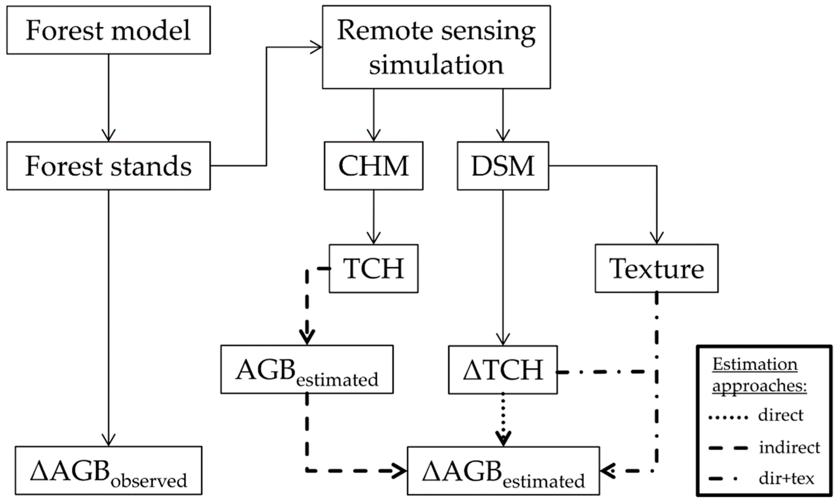
2. Materials and Methods

2.1. Study Area

The study focuses on Barro Colorado Island (BCI), Panama (9.15°N, 79.85°W), a semideciduous tropical lowland rainforest site. Average daily maximum and minimum temperatures are 30.8 and 23.4 °C and the annual precipitation sum is 2600 mm, with a dry season from January to April [55]. Barro Colorado Island hosts a 50 ha (1000 m × 500 m) rainforest observation plot, which has been continuously monitored for more than three decades, with every tree with a diameter at breast height (DBH) ≥1 cm being recorded at 5-year intervals [56,57,58,59]. This inventory dataset with its outstanding spatial and temporal dimensions, along with the large amount of research conducted around it, provides a rich source of information for forest model parameterization [12,60], as well as ground-truthing for remote sensing studies [28,61,62]. In this study, a forest model parameterized with the census data was used and the census data of 2010 and 2015 [in combination with the same allometries as used in the forest model, Equation (3)] served for ground-truthing of satellite-derived estimations of biomass change.

2.2. Forest Model Description

The forest model FORMIND simulates the dynamic processes of establishment, growth, competition (for light and space) and mortality at the individual tree level. Species with similar ecological traits and growth characteristics are grouped into plant functional types (PFT). Biomass growth is mainly driven by light. Large trees receive most of the incoming radiation and shade smaller trees. The resulting biomass growth of each tree is determined by a physiology-based carbon balance, including photosynthesis and respiration. An increase in tree biomass results in stem diameter growth and, through the use of allometric relationships, also in growth of tree height, stem volume and leaf area. A detailed description of the model processes can be found in Fischer et al. [54]. FORMIND was already fully parameterized for the study site [12]. All species present in the BCI plot were grouped into four PFTs, according to stem diameter increment rates (slow, fast) and maximum tree height (small, tall). Allometric equations from the literature [63] were used to describe tree geometries [12]. Tree height H_tree (m) and crown diameter CD_tree (m) are modeled as functions of DBH_tree (m) using Equations (1) and (2).

$${\mathrm{H}}_{\mathrm{tree}}=43.4·{{\mathrm{DBH}}_{\mathrm{tree}}}^{0.6}$$

(1)

$${\mathrm{CD}}_{\mathrm{tree}}=18.2·{{\mathrm{DBH}}_{\mathrm{tree}}}^{0.68}$$

(2)

PFTs can reach different maximal heights (20, 20, 40 and 55 m). AGB_tree is calculated from Equation (3), where F is the stem form factor, which accounts for the deviation from a cylindrical shape, ρ is the wood density (t_ODM m⁻³) and σ is the stem-to-total AGB ratio of the tree. Parameter values are given in Knapp et al. [12].

$${\mathrm{AGB}}_{\mathrm{tree}}=\mathsf{\pi }·{(\frac{{\mathrm{DBH}}_{\mathrm{tree}}}{2})}^2·{\mathrm{H}}_{\mathrm{tree}}·\mathrm{F}·\frac{\mathsf{\rho }}{\mathsf{\sigma }}$$

(3)

The parameterization has been shown to reproduce several patterns observed in the field (AGB, basal area, stem numbers and stem size distributions of the total plot and per PFT). Additionally, it has been used in combination with lidar simulations and could reproduce patterns of airborne lidar data [12]. The temporal development of AGB and canopy height during primary succession is shown in the Appendix A (Figure A1).

2.3. Simulations

FORMIND was used to simulate the development of a 16 ha area (400 m × 400 m) of the BCI forest for a long period (2000 years). The first 200 years of spin-up were discarded from the analysis. In each year, a full inventory table containing all trees with DBH ≥ 3 cm was stored and a virtual lidar scan of the area was sampled using the lidar simulation approach described by Knapp et al. [12] (Figure 1). In FORMIND, we simulated spatially explicit disturbances to frequently clear parts of the area. Disturbances were set to reoccur at random times and places within the area with an average time interval of 25 years and an average affected area of 50% [54]. These settings created a spatially heterogeneous mosaic of different forest regrowth stages. The scenario was designed to produce a dataset with maximum possible structural heterogeneity to cover the full range of possible biomass and height changes with the simulations.

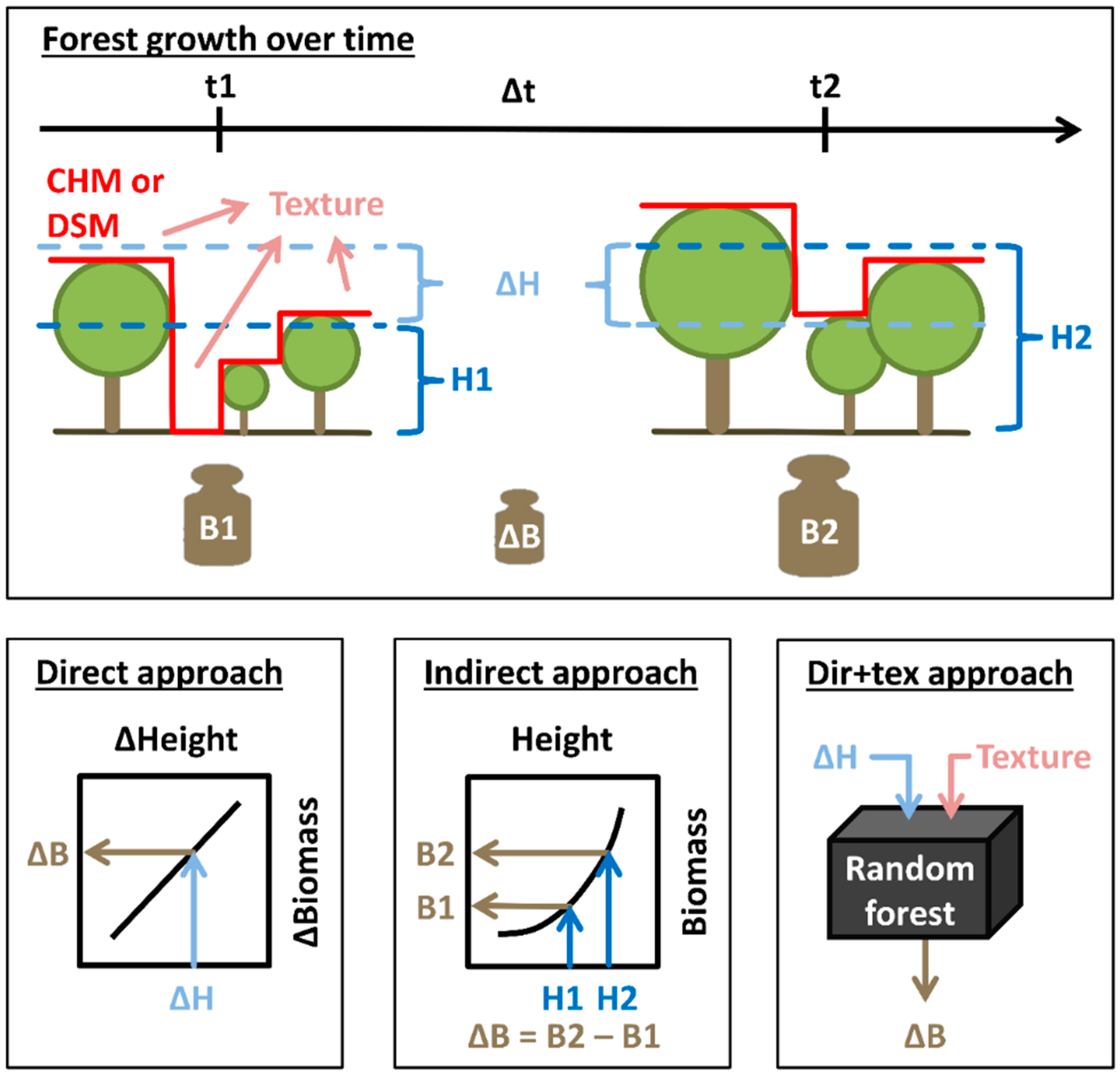
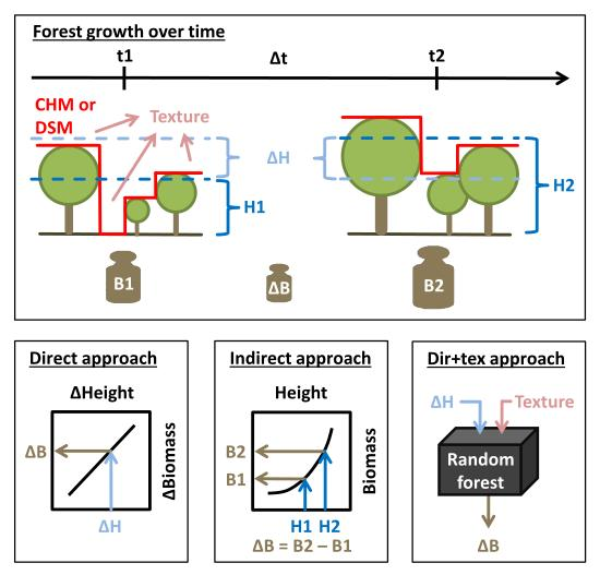
2.4. Biomass, Height and Change Calculations

The simulated lidar data were processed to obtain a metric called TCH10 (mean top-of-canopy height with 10 m pixel resolution) at 1 ha scale. This metric has been shown to yield a height-to-biomass relationship which produces accurate biomass stock estimates (root mean squared error, RMSE = 19.8 t ha⁻¹; nRMSE = 8%; R² = 0.96; [12]). To obtain TCH10 from the simulated lidar point cloud, CHM was produced by taking the height of the highest lidar return falling into each 10 m × 10 m area as pixel value. Next, all pixel values were averaged to obtain one TCH10 value for each hectare. AGB of the simulated forest stands was aggregated at the 1 ha scale. Changes in observed AGB (called ΔAGB_observed) and changes in TCH10 (called ΔTCH10) over each 5-year interval were calculated for each simulated hectare (Figure 1, see Appendix A for equivalent analysis for 10- and 25-year intervals). The total number of analyzed 1 ha forest-stands was 28,736.

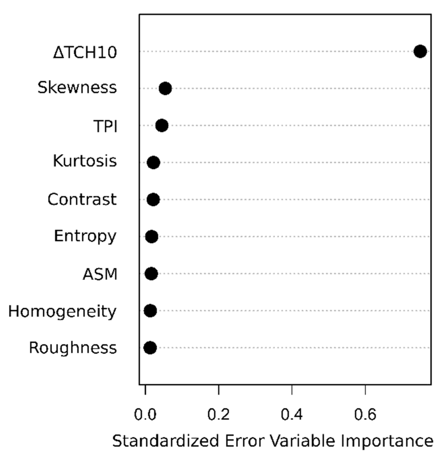
2.5. Texture Calculations

A variety of texture metrics were derived from the simulated CHM rasters (10 m resolution) to capture vegetation surface variability. We used a 3 × 3 pixel moving window (30 m × 30 m), only considering the direct neighbors for each pixel, and then averaged those textures over each hectare. First-order texture metrics are independent of the spatial arrangement of pixel values within the moving window. The following first-order texture metrics were derived (using the raster package in R [64]): standard deviation, skewness, kurtosis, slope, topographic ruggedness index (TRI), topographic position index (TPI) and roughness of the nine pixel values in the moving window. Second-order texture metrics are based on the grey-level co-occurrence matrix (GLCM)—in other words, they consider how often certain pixel values occur next to each other [65]. To obtain a limited set of discrete grey-levels for GLCM texture calculations, the original CHM values were rounded (5 m classes). The following GLCM metrics were calculated (using the glcm package in R): homogeneity, contrast, dissimilarity, entropy and angular second moment (ASM). Directionality in the co-occurrence pattern was not considered (circular version). It is important to note that all texture metrics are independent of the absolute pixel values. The texture metrics depend only on the differences in values between focal pixel and neighbor pixels. Thus, they can be derived from a CHM (terrain-normalized) or a DSM (not terrain-normalized) alike (assuming that the contribution of terrain variability is much smaller than the contribution of canopy surface variability to DSM variability at the given 30 m × 30 m moving window scale).

2.6. Biomass Change Estimation

Three different approaches for ΔAGB estimation were tested with the simulated dataset: (i) the direct approach; (ii) the indirect approach and (iii) an enhanced direct approach involving canopy texture information (dir+tex, Figure 2).

2.6.1. Direct Approach

A linear regression model with slope m and intercept n was fit between simulation-derived ΔAGB_observed and ΔTCH10 (Equation (4)) and used for ΔAGB_direct predictions.

$$\Delta {\mathrm{AGB}}_{\mathrm{direct}}=\mathrm{m}·\Delta \mathrm{TCH}10+\mathrm{n}$$

(4)

2.6.2. Indirect Approach

For each simulated forest stand (1 ha) and simulation year, the AGB stock (t ha⁻¹) was estimated using an established TCH10-to-AGB power law relationship (Equation (5)) with coefficients a = 0.4 and b = 1.81, derived in a previous study [12].

$$\mathrm{AGB}=\mathrm{a}·\mathrm{TCH}{10}^{\mathrm{b}}$$

(5)

ΔAGB_indirect was calculated as the difference between AGB stocks at the beginning (t1) and end (t2) of the time interval [Equation (6)].

$$\Delta {\mathrm{AGB}}_{\mathrm{indirect}}={\mathrm{AGB}}_{\mathrm{t}2}-{\mathrm{AGB}}_{\mathrm{t}1}=\mathrm{a}·{\mathrm{TCH}{10}_{\mathrm{t}2}}^{\mathrm{b}}-\mathrm{a}·{\mathrm{TCH}{10}_{\mathrm{t}1}}^{\mathrm{b}}$$

(6)

2.6.3. Enhanced Direct Approach (Dir+Tex)

We used the random forest machine learning algorithm [66] to predict ΔAGB_dir+tex from ΔTCH10 (like in the direct approach) in combination with the CHM texture metrics. Random forest is an ensemble method based on regression trees. To train the algorithm, an ensemble of regression trees (here, 1000) is fit. Each single tree is trained using only a subset of the full training data and using only a subset of available predictor variables. A prediction of a random forest is generated by averaging the predictions obtained from all single regression trees. We used the model selection procedure developed by Murphy et al. [67] to obtain a parsimonious set of a few meaningful predictor variables (using the rfUtilities package in R). The goal of the procedure is to find the model that maximizes explained variability, minimizes the mean squared error (MSE) and needs the lowest possible number of predictor variables. In the procedure, random forest models are iteratively fit to the data, starting with all predictor variables. During each iteration, predictors are ranked by decreasing relative importance (contribution to MSE reduction), and predictors falling below an importance threshold are dropped before the next iteration. We used deciles from 0.1 to 1 as importance thresholds. Additionally, we chose a parsimony threshold of 0.05, meaning that in the end, from all models for which MSE was only 5% or less above the MSE of the very best model, the model with the smallest number of predictors was chosen as the most parsimonious and hence best model. The model selection was applied using the whole dataset.

The three different approaches for ΔAGB prediction were evaluated based on how well predictions fit observations (i.e., ΔAGB_observed derived directly from the FORMIND output) and corresponding goodness-of-fit statistics, such as R², RMSE and bias (mean residual value). To avoid overfitting of the machine learning model in the dir+tex approach, the dataset was split into five similarly sized groups, and five random forest models were trained with 80% of the data, respectively. The predictions were then made for the remaining 20% test data, which were not part of the training dataset (5-fold cross-validation).

2.7. Evaluation Experiments by Bootstrapping

To assess how prediction accuracy depends on forest height, we conducted a bootstrapping analysis of the simulated dataset. We iterated through forest height classes i from 5 to 50 m in 1 m steps. For each height class i, the simulated dataset was subset, selecting all stands for which the stand height at the initial year (TCH10_t1) was inside the height class i with a class width of 10 m (i.e., i − 5 m < TCH10_t1 < i + 5 m). From all available stands in each height class i, 1000 stands were randomly sampled with replacement. Estimations of ΔAGB were derived for the 1000 sample stands using (i) the indirect; (ii) the direct and (iii) the dir+tex approach. These ΔAGB estimates were compared against the actual ΔAGB_observed values of each stand to calculate and record R², RMSE and bias. The whole sampling procedure was repeated 100 times for each height class.

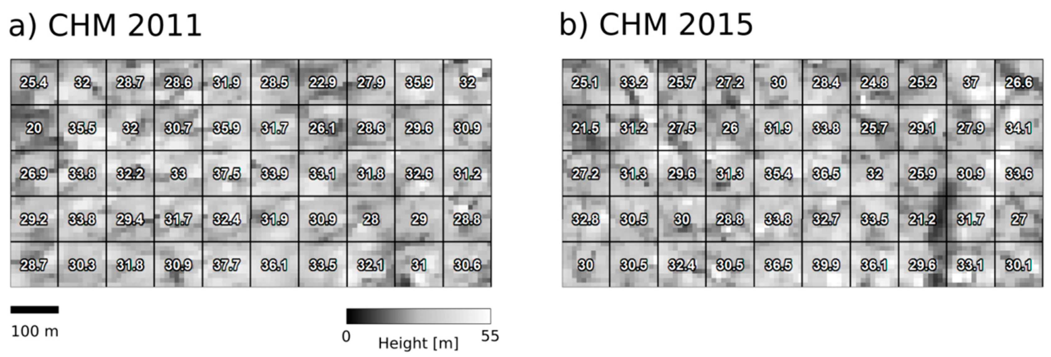
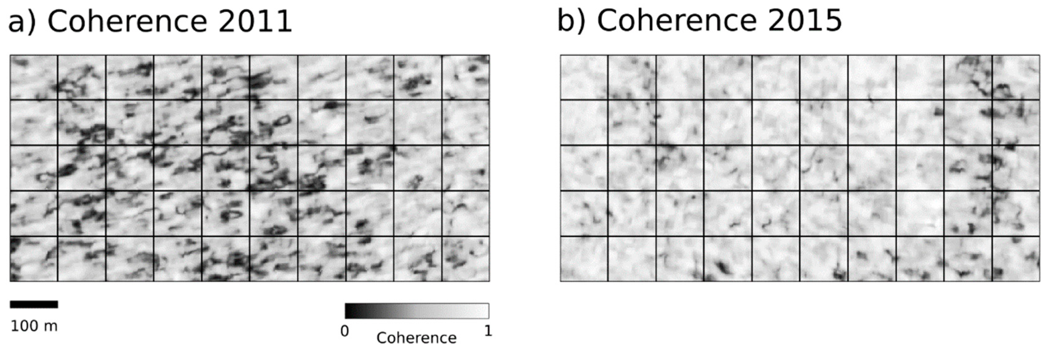
2.8. Application on TanDEM-X Data

To finally test the derived models on real world data, we used imagery derived from the TanDEM-X satellites over BCI in the years 2011 and 2015. TanDEM-X is a radar interferometer with SAR providing single-pass interferometric [68,69] and polarimetric interferometric [70] data at X-band [71]. The data have been acquired in a bistatic configuration, with a practically zero temporal baseline and a spatial baseline corresponding to a height of ambiguity of about 47 m for the 2011 and 70 m for the 2015 acquisition. Canopy height was calculated from interferometric TanDEM-X data at HH polarization (horizontal transmit and horizontal receive) in combination with a lidar DTM (acquired in 2009 [12,62]) needed as reference for the terrain topography below the trees. The single inversion steps are described in detail in Kugler et al. [72]. Here, the Single-Pol Inversion was applied. The forest layer was modeled as a random volume (random distribution of scatterers) over a ground layer, as described by Attema and Ulaby [73] and Treuhaft et al. [74]. This random volume over ground model (RVoG) assumes that the backscattering at X-band along forest height can then be described by an exponential backscatter function in which the backscattered power decreases from the tree tops to the ground. Furthermore, Kugler et al. [72] assumed that the interferometric measurement at X-band contains only backscattering from the vegetation layer (no backscattering from the ground below the forest). With these preconditions and with the ground information from the lidar DTM, we constructed CHMs of 10 m resolution from the TanDEM-X data for the years 2011 and 2015. TCH10 was derived at 1 ha scale for the 50 ha inventory plot for both years. ΔAGB was estimated from ΔTCH10 using the three approaches. As ground-truth, AGB at 1 ha scale was calculated from DBH measurements of the BCI census data of 2010 and 2015 using the same tree allometries as in FORMIND [Equation (3)]. Inventory-based ΔAGB was compared against the three TanDEM-X-based ΔAGB estimates.

3. Results

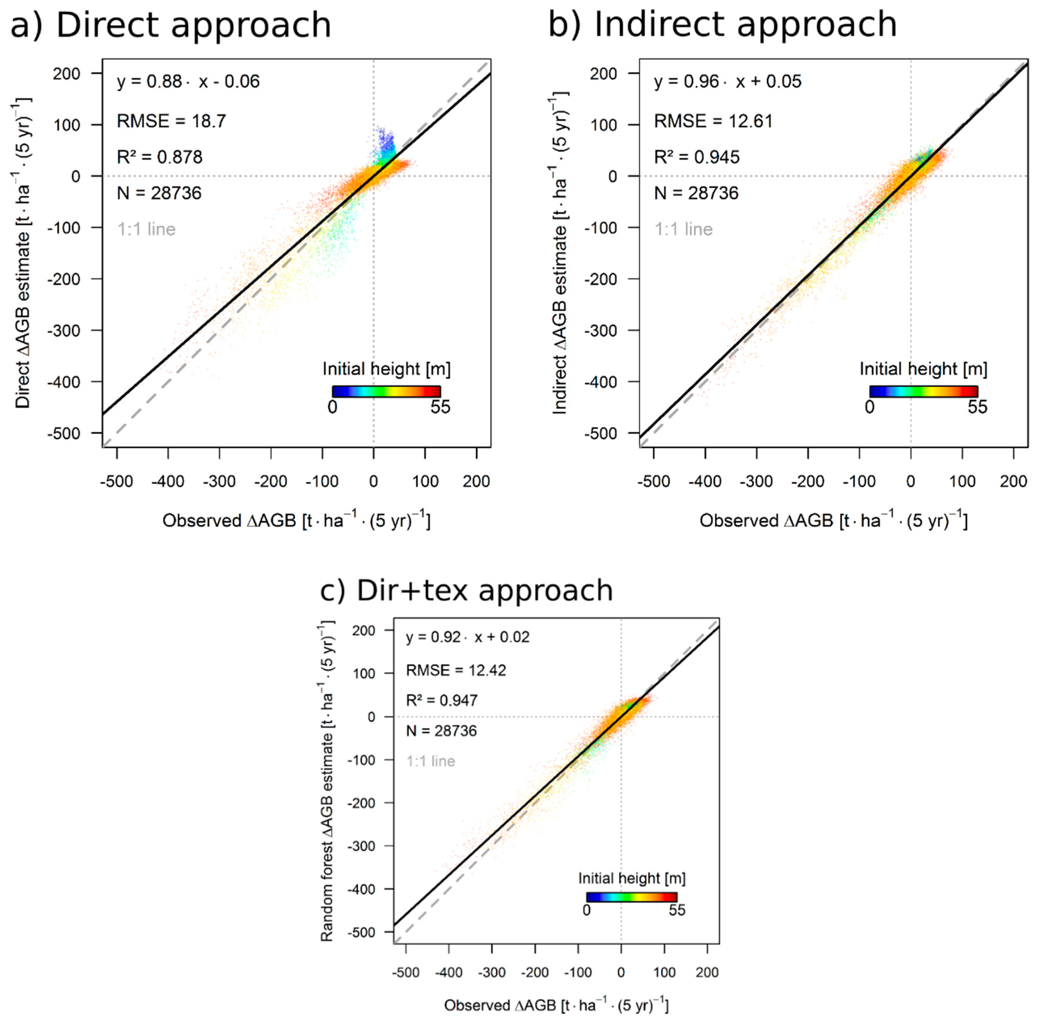
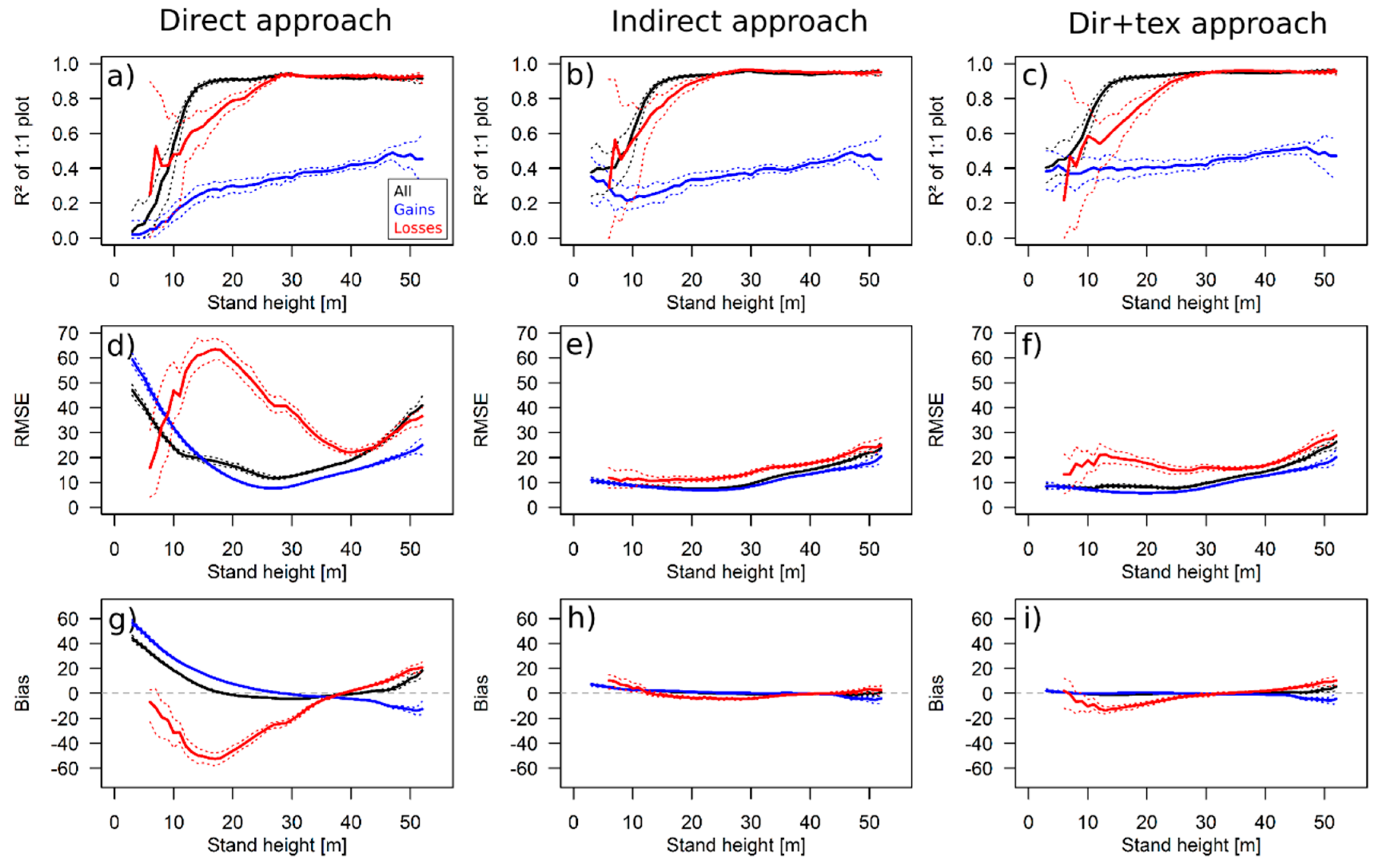
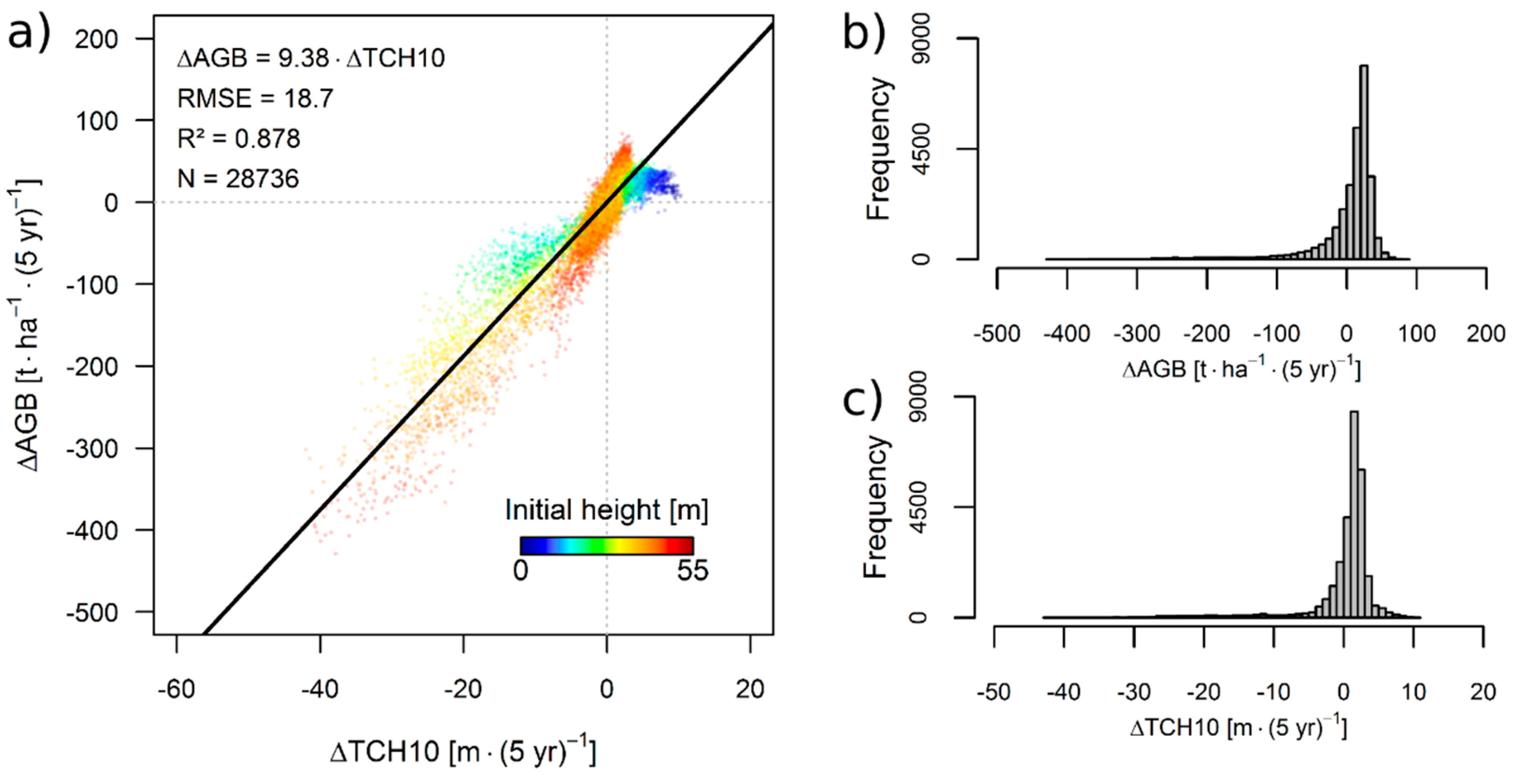
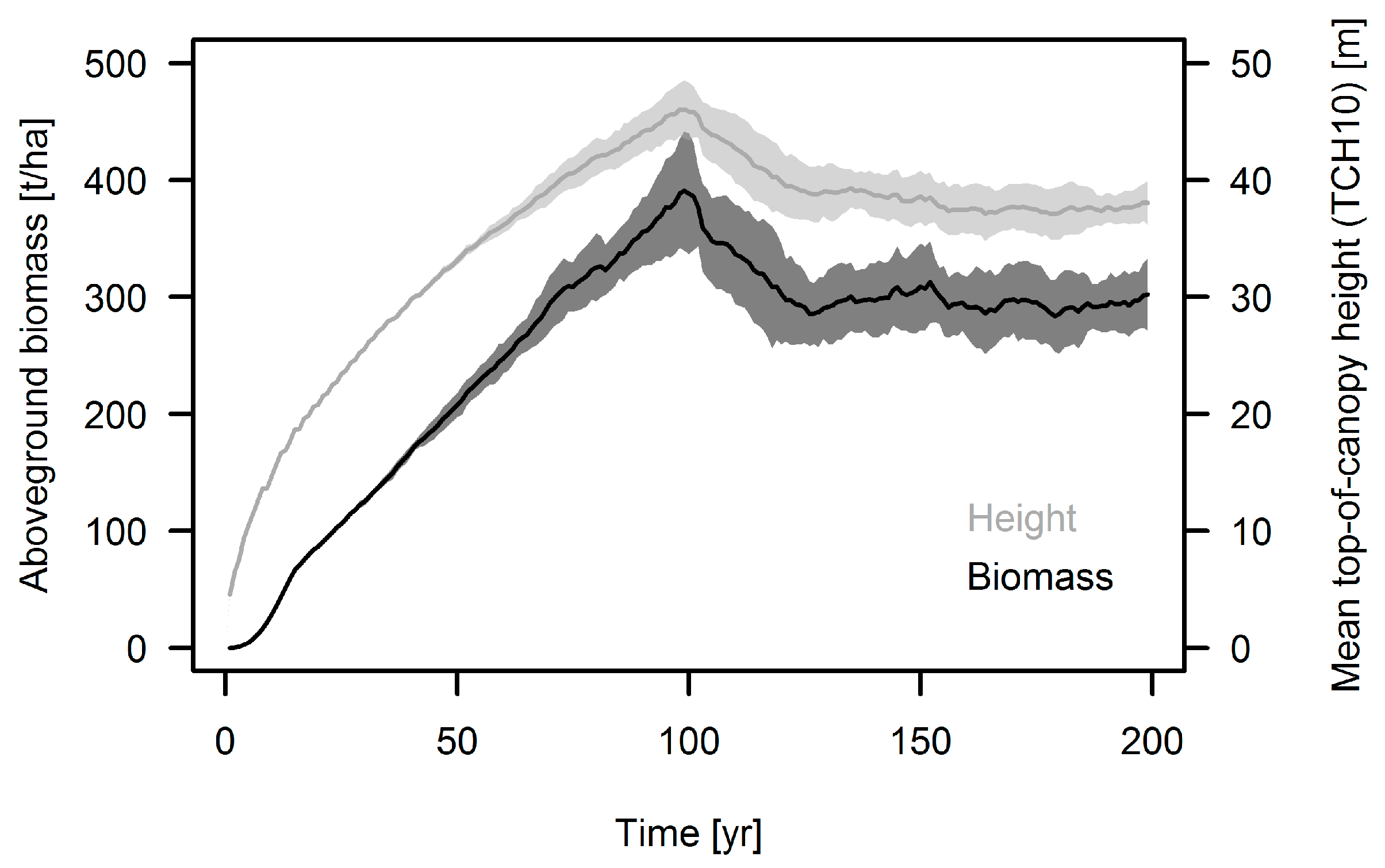
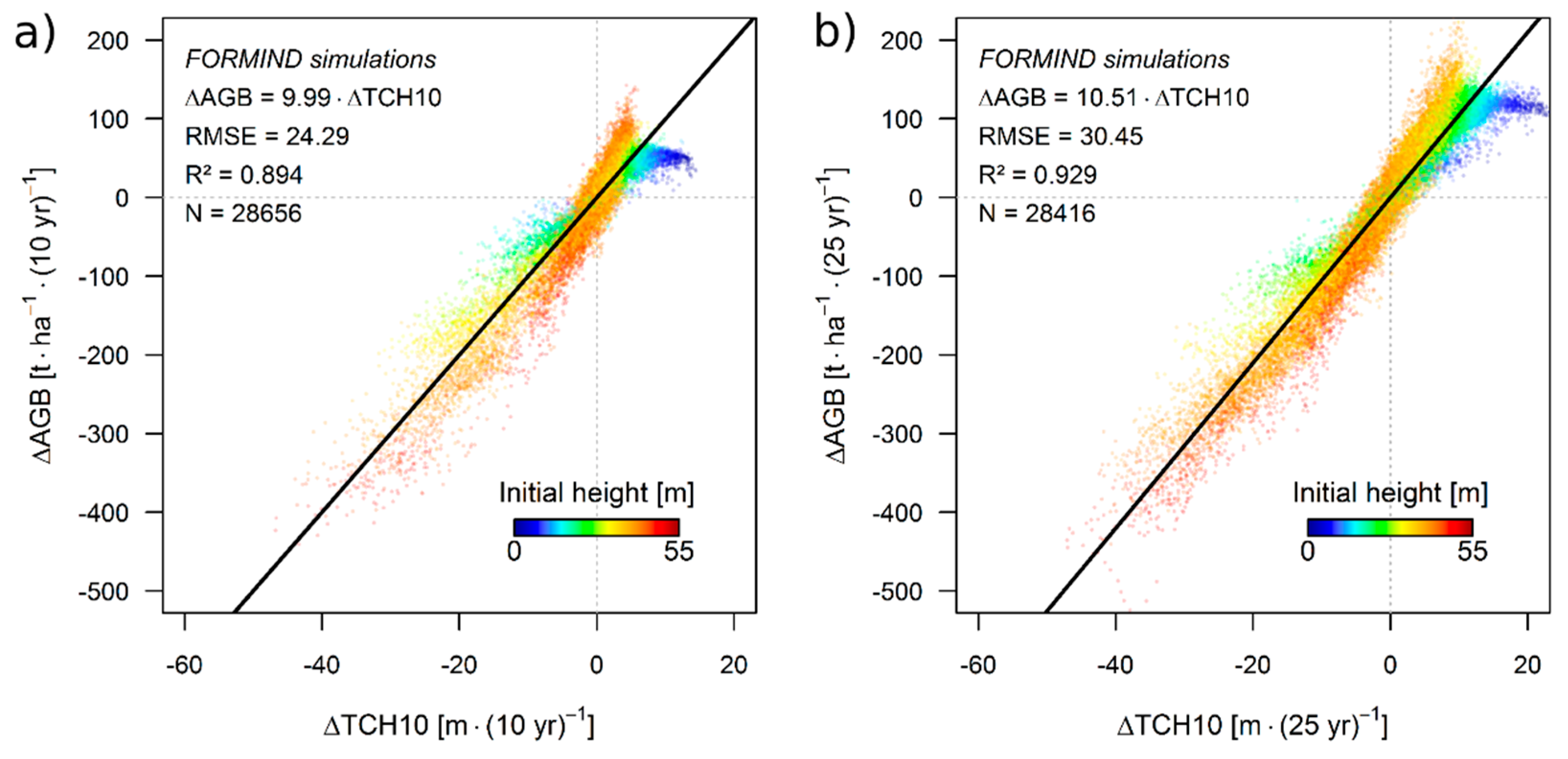
3.1. Simulation Results

In total, the simulated forest dataset consisted of 28,736 ha. For each of these 1 ha stands, the changes in biomass and height were recorded over a 5-year interval. Biomass increased on 72.6% (20,868 ha) and decreased on 27.4% (7868 ha) of the stands. Height increased on 74.9% (21,522 ha), decreased on 25% (7186 ha) and stayed equal on 0.1% (28 ha) of the stands. The maximal biomass gain was 83.7 t ha⁻¹ and the maximal biomass loss was −428.6 t ha⁻¹. The maximal height gain was 10.3 m and the maximal height loss was −42.6 m.

To establish a direct relationship between height change ΔTCH10 and biomass change ΔAGB, a linear regression model was fit between the two variables (Figure 3) with a significant slope term of 9.38 (p < 0.001) and an insignificant intercept of 0.14 (p = 0.218). This matches the expectation that a change of zero in forest height should, on average, also result in zero change in biomass. Forcing the regression through the origin did not change the slope term. The R² was 0.878 and the RMSE was 18.7 t ha⁻¹ (5 year)⁻¹. Figure 3 shows the scatterplot, with colors indicating the TCH10 of each stand at the initial year. Low, early successional stands (blue) tend to show large ΔTCH10 values associated with small ΔAGB values, whereas high, old-growth forests (red) tend to show small ΔTCH10 values associated with large ΔAGB values. Results for the analyses of 10- and 25-year time intervals can be found in Appendix A (Figure A2).

The derived ΔTCH10-to-ΔAGB relationship was used to estimate ΔAGB from ΔTCH10 following the direct approach. Alternatively, ΔAGB was estimated for each hectare following the indirect approach and the dir+tex approach. Statistics were derived for the linear relationship of prediction vs. observation. The direct approach resulted in R² = 0.878 (RMSE = 18.7 t ha⁻¹ (5 year)⁻¹). The indirect approach resulted in a R² = 0.945 (RMSE = 12.61 t ha⁻¹ (5 year)⁻¹). The cross-validation of the dir+tex approach resulted in a R² = 0.947 (RMSE = 12.42 t ha⁻¹ (5 year)⁻¹). Figure 4 shows the 1:1-plots for the different approaches.

In the random forest model selection procedure for the dir+tex approach, nine predictor variables were selected to form the most parsimonious model (Figure A3, Appendix A). ΔTCH10 was identified clearly as the most important predictor variable, followed by first-order texture variables skewness, topographic position index and kurtosis. Second-order (GLCM-based) texture metrics were of minor importance.

The derived models for ΔAGB estimation were evaluated for forests with different heights (bootstrapping analysis). We explored height gains and losses separately (Figure 5). According to the R² values (Figure 5a–c), the linear trend between prediction and observation is weak for stands with low canopy heights (TCH10 < 10 m) but the R² values reach around 0.9 for all stands with TCH10 ≥ 10 m. However, if losses are regarded separately, stands need to have an initial height ≥ 25 m to show such high R² values. If gains are regarded separately, the linear trend is generally less pronounced, with maximal observed R² values being around 0.5. Overall, the R² patterns are similar for the direct, the indirect and the dir+tex approach with a slight increase from low to high stands.

In contrast to the R² patterns, RMSE patterns are quite distinct among the approaches. RMSE values for the direct approach (Figure 5d) are large for low and high stands and have a minimum at intermediate stand heights around 25 m (40 m in case of losses). For the indirect approach (Figure 5e), RMSE values stay constant at around 10 t for stands with heights < 30 m and increase slightly for stands with heights ≥ 30 m. For the dir+tex approach (Figure 5f), the RMSE pattern for gains is similar to the indirect approach. For losses, the pattern is similar to the direct approach but with smaller RMSE values.

Finally, when we look at the systematic biases of the ΔAGB predictions, the indirect approach does not show any pronounced bias over the entire height range (Figure 5h). The direct approach leads to considerable systematic biases when estimating ΔAGB from height gains and losses (Figure 5g). Gains are overestimated by up to 60 t for the lowest forest stands and underestimated by up to −20 t for the highest stands. Losses are negatively biased by up to −50 t for low stands and positively biased by up to 20 t for high stands. The biases are around zero for stands around 35 m height. The biases for the dir+tex approach are higher than the ones for the indirect approach but much lower than the ones for the direct approach (Figure 5i). Gains are unbiased for stands up to 40 m height. Biases of losses show a similar but less pronounced pattern to the direct approach.

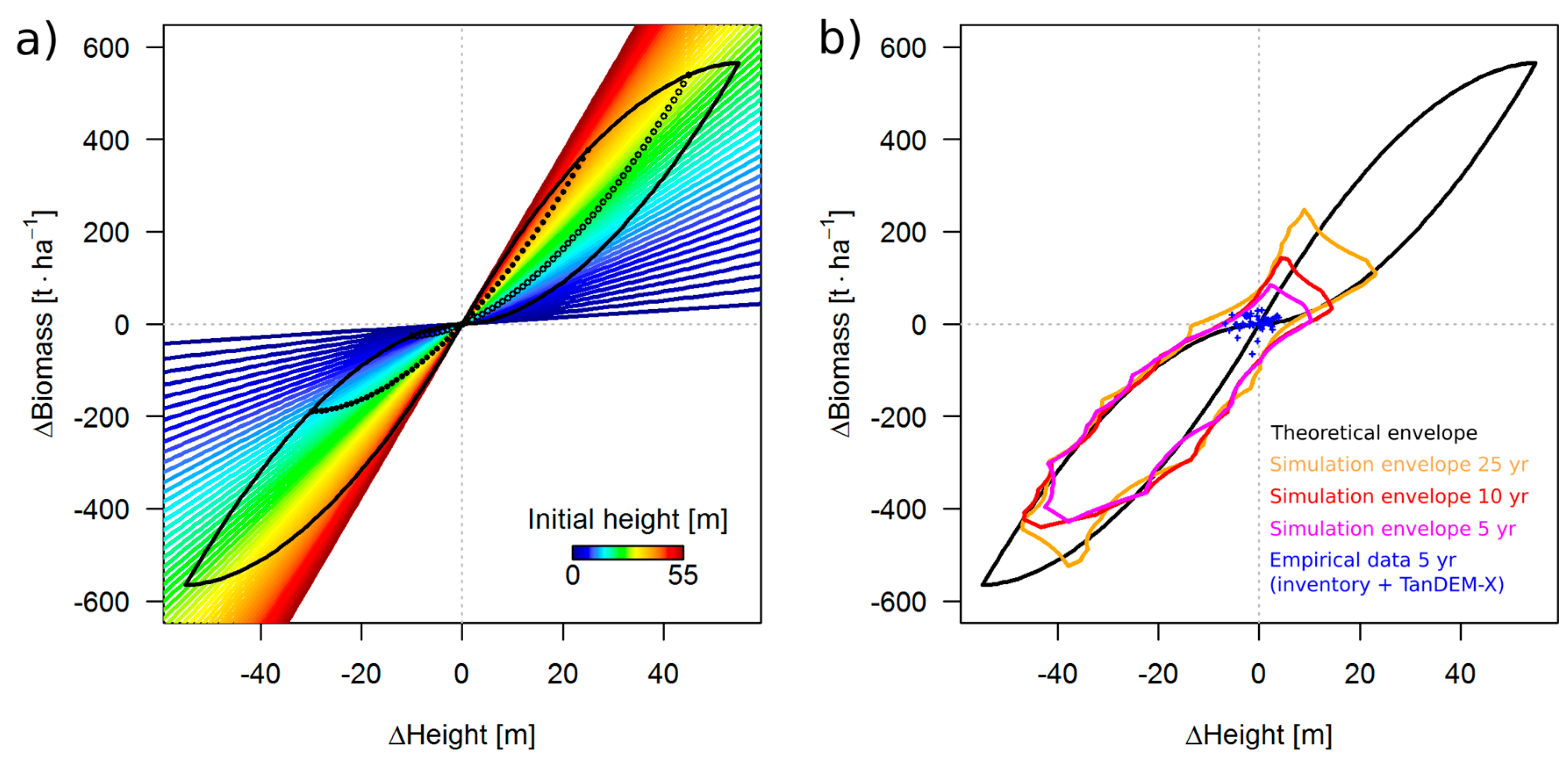
3.2. Theoretical Considerations about the ΔH-to-ΔAGB Relationship

For a better understanding of the observed biases, in particular, the height-dependent biases of the direct approach, we made the following theoretical considerations. For simplicity, we replaced TCH10 with H. The problem with assuming a linear relationship between ΔH and ΔAGB is that the underlying H-to-AGB relationship is nonlinear and can be described, for example, by a power law (Equation (7) with parameters a and b from Equation (5)). The relationship between height change and biomass change at any given height can be derived from the first derivative of Equation (7) (see Equations (8) and (9)).

$$\mathrm{AGB}=\mathrm{a}·{\mathrm{H}}^{\mathrm{b}}$$

(7)

$$\frac{\mathrm{dAGB}}{\mathrm{dH}}=\mathrm{a}·\mathrm{b}·{\mathrm{H}}^{\mathrm{b}-1}$$

(8)

$$\Delta \mathrm{AGB}=\mathrm{a}·\mathrm{b}·{\mathrm{H}}^{\mathrm{b}-1}·\Delta \mathrm{H}$$

(9)

Equation (9) describes the relationship between ΔAGB and ΔH, which depends also on H (which is unknown in case of missing DTM). Thus, the magnitude of ΔAGB is not only dependent on ΔH, but also on the absolute height H of a stand. For any given stand height H, the ΔH-to-ΔAGB relationship can be expressed with a linear model, but the slope of the linear model is different for each possible H (Figure 6a). If we assume that H lies inside the range from 0 to 55 m, the marked area in the plot encloses all possible ΔH–ΔAGB combinations (black envelope resembling the shape of a propeller). Stands of a given initial height move along power law-shaped trajectories over time (e.g., open circles for 10 m and filled circles for 30 m initial height in Figure 6a). The possible gains for a certain time interval are constrained by the forest’s growth rate, while losses can be large even within short time periods, due to the stochastic occurrence of mortality and disturbance events. For 5-, 10- and 25-year intervals, the simulations show the subspace of observable ΔH–ΔAGB combinations (colored envelopes in Figure 6b). The simulation data exceed the black propeller, particularly around the coordinate origin. The explanation is that the black propeller envelope only applies under the assumption of an exact power law relationship between H and AGB without variability in the H-to-AGB relationship.

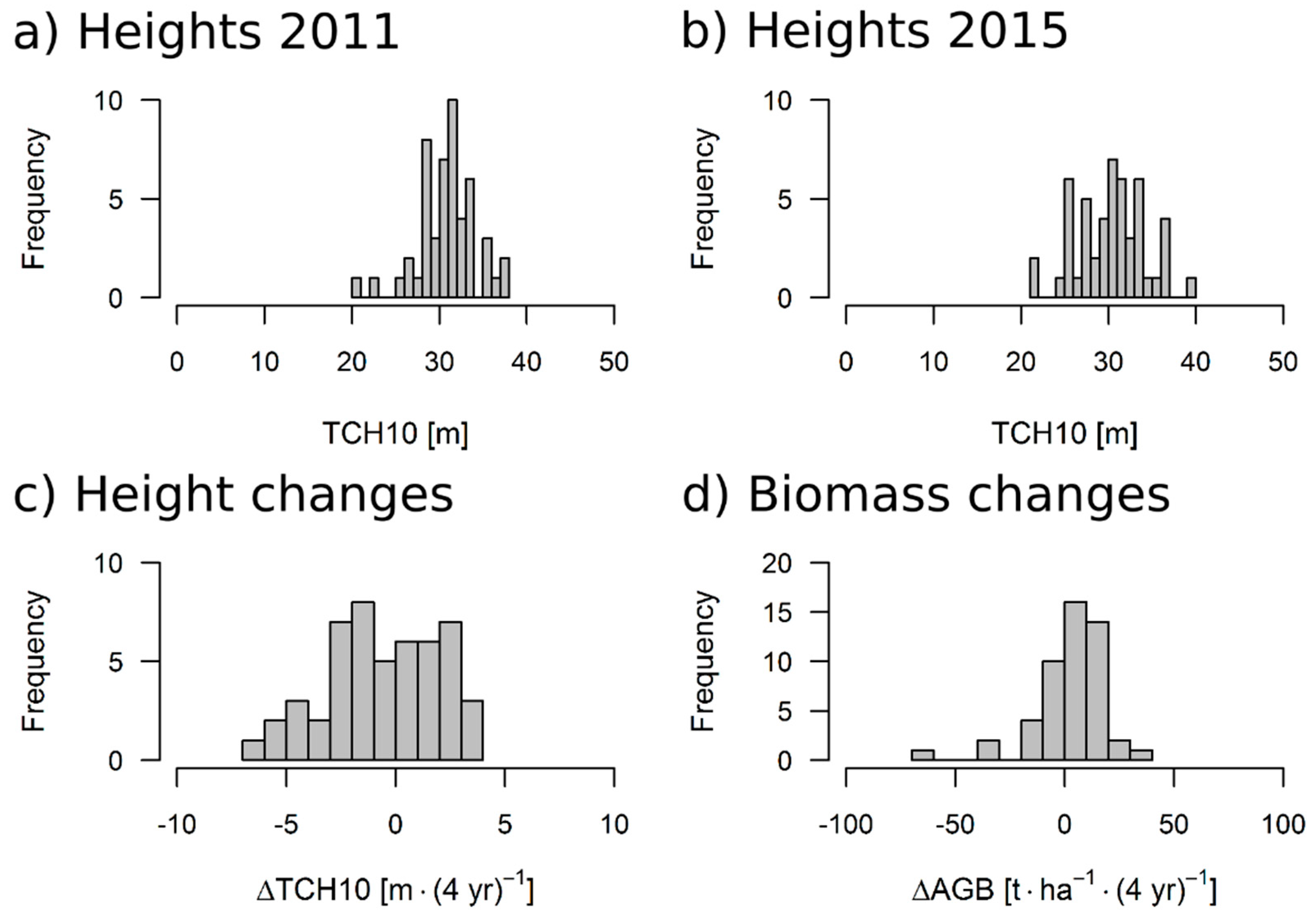
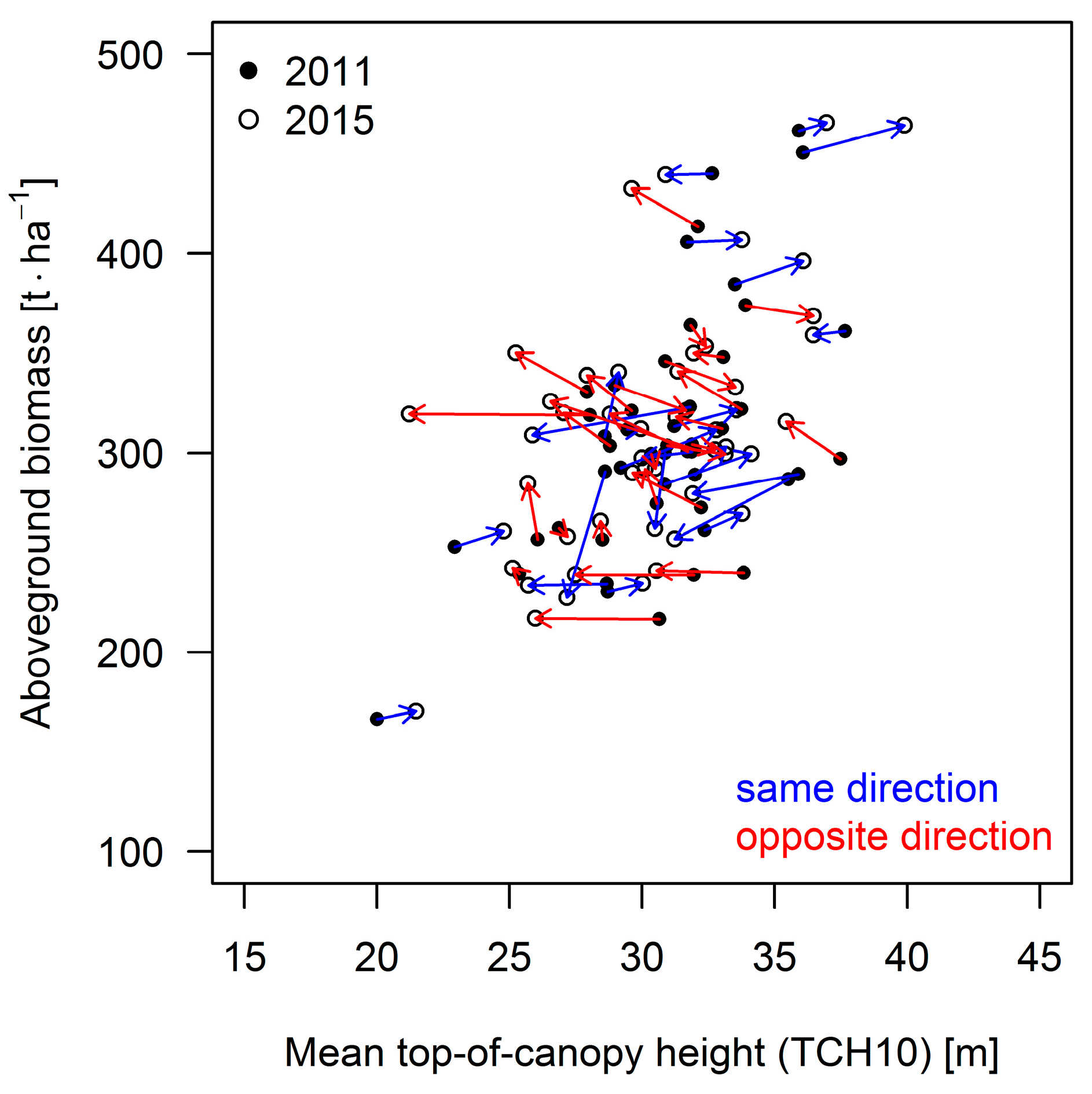
3.3. Results for the 50 ha Plot

The CHMs of the BCI 50 ha plot derived from TanDEM-X data of 2011 and 2015 (Figure A4, Appendix A) served to test the three ΔAGB estimation models which had been fit with simulation data. At the 1 ha scale, the mean TCH10 over the 50 ha was 31.0 m (± 3.4 m SD) in 2011 and 30.3 m (±3.9 m SD) in 2015. Distributions of canopy height (TCH10) in both years and canopy height change (ΔTCH10) within the 4 years are given in Figure 7a–c. The distribution of biomass change (ΔAGB) calculated from the inventory data is given in Figure 7d. There was a slight loss in average canopy height (mean ΔTCH10 = −0.6 m ± 2.6 m SD), but a slight gain in average biomass (mean ΔAGB = 3.3 t ha⁻¹ ± 16.6 t ha⁻¹ SD). When plotted against each other, ΔAGB and ΔTCH10 of the BCI plot scatter closely around the coordinate origin in Figure 6b (blue points), showing neither strong gains nor losses.

The TanDEM-X-derived ΔAGB estimates from all three approaches did not show any significant correlation with the observed ΔAGB derived from the forest inventory data from censuses in 2010 and 2015, with R² values close to zero (Figure 8 and

Table 1. R² values for the 1:1 relationships of ΔAGB predictions from TanDEM-X data following the three different approaches vs. inventory-based ΔAGB and against each other.

	Direct	Indirect	Dir+Tex
Inventory	0.006	0.007	0.003
Dir+Tex	0.966	0.946	-
Indirect	0.991	-	-

). The estimates of ΔAGB from the three approaches were, however, closely correlated among each other with R² values ≥ 0.96 (Table 1). Thus, within the narrow range of height changes observed in the BCI plot over the short time interval of 4 years, the three different approaches produced very similar predictions. However, the observed height changes do not reflect the changes in AGB adequately, hence, none of the approaches resulted in ΔAGB estimates that could be confirmed by the ground-truth data.

Figure 9 shows ABG stocks plotted over TCH10 at 1 ha scale for both years. The arrows illustrate the changes between 2011 and 2015 in both attributes. There is no clear link in the sense that an increase or decrease in AGB is accompanied with an increase or decrease of canopy height, respectively. On 23 hectares, AGB and canopy height changed in the same direction, whereas on the remaining 27 hectares they changed in opposite directions. This explains the difficulties in estimating ΔAGB.

4. Discussion

Our results provide insight into the relationship between canopy height and biomass change over time for a tropical lowland rainforest. Understanding this relationship is crucial to quantify forest carbon losses and gains with remote sensing data. Using forest simulations, including disturbances, we could produce a large dataset covering a wide range of stand structures and successional stages. With this dataset, we were able to compare the performance of three different approaches to estimate biomass change.

4.1. Performance of the Approaches

In comparison, the indirect approach performed better than the direct approach. The former led to more precise and unbiased ΔAGB estimations over the full range of possible height changes. Nevertheless, looking only at the statistics for the whole dataset, both approaches showed high R² values. However, the colors indicating the initial height in the 1:1-plot (Figure 4a) and the bootstrapping results (Figure 5) reveal that the direct approach only worked well in a window of forest heights around 30 m, while for low and high stands it produced strongly biased results. Analyzing gains and losses further revealed the asymmetry in the ΔH–ΔAGB relationship, due to slow, continuous growth and abrupt, stochastic mortality, and its effect on statistics that quantify prediction accuracy. The biases of the direct approach for low and high stands can be explained by the nonlinearity of the H–AGB relationship, leading to different slopes in the ΔH–ΔAGB relationship, depending on stand height. The development of an enhanced direct approach, which avoids such bias and allows accurate estimations, even in the absence of information about H, was the goal behind the dir+tex approach. The textural information should compensate for the missing information about H. It was shown that estimations of ΔAGB from the dir+tex approach were nearly as unbiased and of similar accuracy to those from the indirect approach.

In this study, we did not test the robustness of the approaches with regard to the time interval, that is, whether it is possible to calibrate an approach based on observations over a certain time interval and then apply it for predictions over a different time interval. For the indirect approach, the interval is irrelevant, because it is based on two independent biomass stock estimates. For the direct approach, estimates depend on the slope of the ΔH–ΔAGB relationship, which was similar for 5-, 10- and 25-year intervals (9.38, 9.99, 10.51). In the dir+tex approach, the only variable depending on the interval is ΔH (like in the direct approach), while all texture variables only describe the state of the forest at the initial point of the interval. Hence, we expect all three approaches to be fairly robust for variable time intervals. The length of the time interval does, however, influence the frequency distribution of observable changes, with large gains being only possible over longer time intervals and large losses being more frequent over longer time intervals (Figure A2).

4.2. Comparison with Other Studies

In an earlier study comparing the indirect and direct approach on BCI, Meyer et al. [28] used data acquired in 1998 with the Laser Vegetation Imaging Sensor (LVIS, large footprint) and discrete return small footprint lidar data from 2009 (11-year interval). They could not find a direct ΔH–ΔAGB relationship at the 1 ha scale (R² < 0.1) and using the indirect approach they reported large estimation uncertainties. They considered the different sensor types as a major reason for the missing direct ΔH–ΔAGB relationship. In another study using data from two successive LVIS campaigns in 1998 and 2005 (7-year interval) at La Selva, Costa Rica, Dubayah et al. [27] found a direct ΔH–ΔAGB relationship (R² = 0.65, RSE = 10.54 t ha⁻¹ or excluding secondary forests R² = 0.5, RSE = 8.86 t ha⁻¹) using a two-predictor model based on changes in height quantiles ΔRH50 and ΔRH100. The statistics of that relationship are in the order of magnitude of what was observed for gains in our simulations. Several comparative studies in boreal [24,75] and subtropical [23] forests reported ΔAGB estimations to be more accurate when obtained from the direct approach as opposed to the indirect approach. Others, covering tropical Asia [76] or temperate North America [25], only tested the indirect approach. In two studies, we found scatterplots that indicate a different slope in the ΔH–ΔAGB relationship for secondary (disturbed) sites than for old-growth (undisturbed) sites (Figure 8 in [27] and Figure 9F in [25]). This is in agreement with our simulation results and the explanation given in Figure 6.

As soon as the goal is to cover a wide range of successional stages, including disturbed stands, the nonlinear H–AGB relationship leads to H-dependent biases in the linear ΔH–ΔAGB relationship. The condition for an unbiased direct approach would be that the underlying H–AGB relationship is linear. In past studies, the direct approach has worked better in boreal sites (coniferous forests) and worse in tropical sites (broadleaved forests). Hence, the differences in crown shapes and forest structure between those forest types might lead to a more linear H–AGB relationship in coniferous forests, making them more suitable for the direct approach.

Recently, there have been attempts to generalize the height-to-biomass relationships, accounting for differences between geographical regions and forest types [15,77]. These relationships are, however, not linear, but power laws. Thus, the linear relationship that has been found in some studies in the past might be an effect of either small plot sizes, causing large variability [30,78], or a limited sampling of successional stages, not covering the full spectrum of H–AGB combinations.

A linear H–AGB relationship is a strict criterion for the application of a method. Many forests may not fulfill this criterion and for large-scale mapping of AGB changes (from height changes), a method independent of such a requirement should be preferred. With the proposed dir+tex approach, we found a method that works independently of knowledge about absolute canopy height. Biomass changes are estimated based on height change and local canopy texture at the initial point in time. Predictions showed similar accuracies to the indirect approach. Biases were somewhat larger than for the indirect approach but much smaller than for the direct approach. This texture-assisted approach could therefore be applied to multitemporal DSM data for which no exact underlying DTM is available and hence CHM creation is impossible. This applies to global DSMs, originating from different spaceborne sensor systems (SRTM, TanDEM-X) [29,30,31] and to DSMs derived photogrammetrically from digital stereo imagery [37,79].

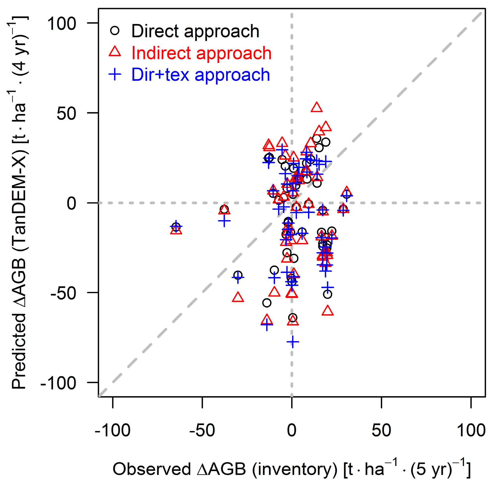
4.3. Outcome of TanDEM-X Application

Despite the good performance of the three approaches on the simulation dataset, none of them were able to produce accurate predictions of biomass change for the BCI 50 ha plot, based on canopy height change derived from TanDEM-X data. The main difference between the simulated data and the TanDEM-X data was that the forest in the simulations was exposed to a disturbance regime causing dramatic changes in canopy height and biomass, while no such disturbances occurred on the BCI plot within the observed time interval. Thus, the changes observed on the BCI plot are only a subset of possible changes for a 5-year interval (Figure 6b). BCI only represents old-growth dynamics with small changes in canopy height and biomass, while the simulations cover the entire range of possible changes. We suspect that there are two main reasons for the difficulties in predicting ΔAGB from TanDEM-X-derived ΔTCH10 on the BCI plot: (i) the variability unexplained by the prediction models and (ii) the uncertainty in canopy height estimates.

Regarding the unexplained variability (i), the bootstrapping results tell us that for an old-growth forest, like on the BCI plot, with an average height TCH10 = 30 m, the average estimation error for ΔAGB over a 5-year interval is around 10 t ha⁻¹ for all three approaches (e.g., for the indirect approach RMSE = 9.5 t ha⁻¹). This is a high uncertainty, given that the standard deviation of ΔAGB from the BCI inventory was only 16.6 t ha⁻¹ and the mean ΔAGB was only 3.3 t ha⁻¹. The high R² values in the direct ΔH–ΔAGB relationship of the simulated data were caused by the large losses. Since such losses did not occur on BCI, the R² for the BCI plot should be expected to be much lower. In the simulations, the average R² for gains only was 0.35 for a 30 m high stand. Even this value can be expected to be too optimistic for the BCI plot, as the simulated gains include areas of recovery after disturbances, which were also not present in the BCI plot. Thus, the intrinsic variability in canopy height and biomass alone leads to a very weak ΔH–ΔAGB relationship for old-growth forests. The simulations did not account for the uncertainty in canopy height estimates from remote sensing, which is yet another factor influencing the results from the BCI plot.

Uncertainty in X-band-derived tropical forest heights (ii) has been reported to lie in a range from 1 to 6 m [72,80]. The precise numbers may vary depending on the sensor configuration, the height metrics and the spatial scale considered. In our study, the main limitation of the TanDEM-X-derived heights arose from the suboptimum spatial baselines available, that were practically too large for the forest heights within the study site, leading to a low interferometric coherence (Figure A5) and to rather inaccurate forest heights. Note that the limited penetration capability at the X-band was circumvented by using lidar-derived topographic information. The observed height changes on the BCI plot were small (standard deviation of 2.6 m for ΔTCH10 at hectare-scale and mean ΔTCH10 of −0.6 m) in comparison to the large uncertainty.

Thus, the two reasons—(i) variability in the ΔH-ΔAGB relationship and (ii) uncertainty in canopy height estimates—lead to a low signal-to-noise ratio and explain why the presented approaches are insufficient for the detection of small changes in AGB in an undisturbed old-growth tropical rainforest. Further sources of uncertainty are the variability in tree geometry at the individual level, which is simplified in the forest model by allometric equations, as well as temporal mismatch (between census and remote sensing acquisition) errors in the census data and geolocation errors.

4.4. Perspectives

The presented approaches to estimate biomass changes at 1 ha scale based on 10 m resolution vegetation height changes are best suited for monitoring changes due to disturbances, degradation and growth. They could serve to map biomass changes caused by these processes from TanDEM-X data at a regional scale. They cannot detect small changes associated with old-growth forest dynamics. Future research efforts should focus on reducing the uncertainty in biomass change estimates. Uncertainty in the prediction models can be reduced—for example, by considering data at finer horizontal resolution, the full vertical signal distribution, the multitude of variables that can describe forest structure and individual-tree-based approaches [26]. The uncertainty in height estimations due to the variability in the remote sensing data can be reduced by fitting trends to dense time series of multiple acquisitions [80]. Future research should also try to disentangle the processes and compartments behind biomass dynamics (including also belowground biomass) by quantifying the contributions of wood productivity, mortality, foliage and fine root turnover [81]. Upcoming spaceborne missions (e.g., GEDI, BIOMASS, Tandem-L) and the increasing data collections from airborne campaigns (lidar, SAR, photogrammetry) will provide the measurements to advance in this direction. Data fusion will help to use the available data most effectively, with each individual mission contributing to a different aspect (e.g., by providing detailed vertical foliage distributions and ground elevation at points in space (GEDI), or wall-to-wall measurements of SAR backscatter from woody biomass components (BIOMASS, Tandem-L)). Forest models will help to understand and interpret new remote sensing observations.

5. Conclusions

In this study, we analyzed different approaches for estimating aboveground biomass change in a tropical rainforest from observed changes in mean top-of-canopy height. With forest simulations, it was possible to generate and analyze data covering a much wider range of changes than is usually available from field data. Goodness-of-fit statistics (R², RMSE and bias) for the ΔAGB estimations were computed over the full range of possible stand heights, also demonstrating an asymmetry between gains and losses. It was found that a direct, linear ΔH-to-ΔAGB relationship only provides accurate predictions under limited conditions and can lead to large prediction biases when applied over a wide range of stand heights. The indirect approach, which builds on the H-to-AGB stock relationship, can be used to avoid such biases, but it is dependent on accurate measurements of canopy height. A third approach, based on random forest machine learning, was found to provide similar prediction accuracies to the indirect approach. The latter did not require canopy height as input. Instead, canopy height change in combination with a set of canopy texture metrics served as predictors. The simulation-derived approaches were not sensitive enough to detect small biomass changes based on TanDEM-X data for a 50 ha plot in Panama. Further research is required to improve our ability to detect even small changes in biomass with remote sensing. The presented approaches with their accuracies of around ±13 t ha⁻¹ are nevertheless well suited for monitoring of forest biomass changes at large scales. In summary, the study demonstrated the potential of using a forest model for improving the understanding and interpretation of multitemporal remote sensing data and for evaluating different approaches.

References

1. Houghton, R.A.; Hall, F.; Goetz, S.J. Importance of biomass in the global carbon cycle. J. Geophys. Res. Biogeosci. 2009, 114, 1–13. [Google Scholar] [CrossRef]
2. Pan, Y.; Birdsey, R.A.; Fang, J.; Houghton, R.; Kauppi, P.E.; Kurz, W.A.; Phillips, O.L.; Shvidenko, A.; Lewis, S.L.; Canadell, J.G.; et al. A Large and Persistent Carbon Sink in the World’s Forests. Science 2011, 333, 988–993. [Google Scholar] [CrossRef] [PubMed]
3. Intergovernmental Panel on Climate Change (IPCC). Climate Change 2007: The Physical Science Basis; IPCC: Geneva, Switzerland, 2007. [Google Scholar]
4. Hansen, M.C.; Potapov, P.V.; Moore, R.; Hancher, M.; Turubanova, S.A.; Tyukavina, A.; Thau, D.; Stehman, S.V.; Goetz, S.J.; Loveland, T.R.; et al. High-resolution global maps of 21st-century forest cover change. Science 2013, 342, 850–853. [Google Scholar] [CrossRef] [PubMed]
5. Zolkos, S.G.; Goetz, S.J.; Dubayah, R. A meta-analysis of terrestrial aboveground biomass estimation using lidar remote sensing. Remote Sens. Environ. 2013, 128, 289–298. [Google Scholar] [CrossRef]
6. Lu, D.; Chen, Q.; Wang, G.; Liu, L.; Li, G.; Moran, E. A survey of remote sensing-based aboveground biomass estimation methods in forest ecosystems. Int. J. Digit. Earth 2014, 1–43. [Google Scholar] [CrossRef]
7. Lefsky, M.A.; Cohen, W.B.; Parker, G.G.; Harding, D.J. Lidar remote sensing for ecosystem studies. Bioscience 2002, 52, 19–30. [Google Scholar] [CrossRef]
8. Wulder, M.A.; White, J.C.; Nelson, R.F.; Næsset, E.; Ørka, H.O.; Coops, N.C.; Hilker, T.; Bater, C.W.; Gobakken, T. Lidar sampling for large-area forest characterization: A review. Remote Sens. Environ. 2012, 121, 196–209. [Google Scholar] [CrossRef]
9. Treuhaft, R.; Gonçalves, F.; Roberto, J.; Keller, M.; Palace, M.; Madsen, S.N.; Sullivan, F.; Graça, P.M.L.A. Tropical-Forest Biomass Estimation at X-Band From the Spaceborne TanDEM-X Interferometer. IEEE Geosci. Remote Sens. Lett. 2015, 12, 239–243. [Google Scholar] [CrossRef] [Green Version]
10. Lefsky, M.A.; Cohen, W.B.; Harding, D.J.; Parker, G.G.; Acker, S.A.; Gower, S.T. Lidar remote sensing of above-ground biomass in three biomes. Glob. Ecol. Biogeogr. 2002, 11, 393–399. [Google Scholar] [CrossRef]
11. Chen, Q.; McRoberts, R.E.; Wang, C.; Radtke, P.J. Forest aboveground biomass mapping and estimation across multiple spatial scales using model-based inference. Remote Sens. Environ. 2016, 184, 350–360. [Google Scholar] [CrossRef]
12. Knapp, N.; Fischer, R.; Huth, A. Linking lidar and forest modeling to assess biomass estimation across scales and disturbance states. Remote Sens. Environ. 2018, 205, 199–209. [Google Scholar] [CrossRef]
13. Fassnacht, F.E.; Hartig, F.; Latifi, H.; Berger, C.; Hernández, J.; Corvalán, P.; Koch, B. Importance of sample size, data type and prediction method for remote sensing-based estimations of aboveground forest biomass. Remote Sens. Environ. 2014, 154, 102–114. [Google Scholar] [CrossRef]
14. Drake, J.B.; Dubayah, R.O.; Clark, D.B.; Knox, R.G.; Blair, J.B.; Hofton, M.A.; Chazdon, R.L.; Weishampel, J.F.; Prince, S. Estimation of tropical forest structural characteristics, using large-footprint lidar. Remote Sens. Environ. 2002, 79, 305–319. [Google Scholar] [CrossRef]
15. Asner, G.P.; Mascaro, J. Mapping tropical forest carbon: Calibrating plot estimates to a simple LiDAR metric. Remote Sens. Environ. 2014, 140, 614–624. [Google Scholar] [CrossRef]
16. Marvin, D.C.; Asner, G.P.; Knapp, D.E.; Anderson, C.B.; Martin, R.E.; Sinca, F.; Tupayachi, R. Amazonian landscapes and the bias in field studies of forest structure and biomass. Proc. Natl. Acad. Sci. USA 2014, 111, E5224–E5232. [Google Scholar] [CrossRef] [PubMed]
17. Getzin, S.; Fischer, R.; Knapp, N.; Huth, A. Using airborne LiDAR to assess spatial heterogeneity in forest structure on Mount Kilimanjaro. Landsc. Ecol. 2017, 32, 1881–1894. [Google Scholar] [CrossRef]
18. Coomes, D.A.; Dalponte, M.; Jucker, T.; Asner, G.P.; Banin, L.F.; Burslem, D.F.R.P.; Lewis, S.L.; Nilus, R.; Phillips, O.L.; Phua, M.H.; et al. Area-based vs. tree-centric approaches to mapping forest carbon in Southeast Asian forests from airborne laser scanning data. Remote Sens. Environ. 2017, 194, 77–88. [Google Scholar] [CrossRef]
19. Asner, G.P.; Knapp, D.E.; Martin, R.E.; Tupayachi, R.; Anderson, C.B.; Mascaro, J.; Sinca, F.; Chadwick, K.D.; Sousan, S.; Higgins, M.; et al. The High-Resolution Carbon Geography of Perú; Minuteman Press: Stanford, CA, USA, 2014. [Google Scholar]
20. Saatchi, S.S.; Harris, N.L.; Brown, S.; Lefsky, M.; Mitchard, E.T.A.; Salas, W.; Zutta, B.R.; Buermann, W.; Lewis, S.L.; Hagen, S.; et al. Benchmark map of forest carbon stocks in tropical regions across three continents. Proc. Natl. Acad. Sci. USA 2011, 108, 9899–9904. [Google Scholar] [CrossRef] [PubMed]
21. Baccini, A.; Goetz, S.J.; Walker, W.S.; Laporte, N.T.; Sun, M.; Sulla-Menashe, D.; Hackler, J.; Beck, P.S.A.; Dubayah, R.; Friedl, M.A.; et al. Estimated carbon dioxide emissions from tropical deforestation improved by carbon-density maps. Nat. Clim. Chang. 2012, 2, 182–185. [Google Scholar] [CrossRef]
22. Harris, N.L.; Brown, S.; Hagen, S.C.; Saatchi, S.S.; Petrova, S.; Salas, W.; Hansen, M.C.; Potapov, P.V.; Lotsch, A. Baseline Map of Carbon Emissions from Deforestation in Tropical Regions. Science 2012, 336, 1573–1576. [Google Scholar] [CrossRef] [PubMed]
23. Cao, L.; Coops, N.C.; Innes, J.L.; Sheppard, S.R.J.; Fu, L.; Ruan, H.; She, G. Estimation of forest biomass dynamics in subtropical forests using multi-temporal airborne LiDAR data. Remote Sens. Environ. 2016, 178, 158–171. [Google Scholar] [CrossRef]
24. Bollandsås, O.M.; Gregoire, T.G.; Næsset, E.; Øyen, B.H. Detection of biomass change in a Norwegian mountain forest area using small footprint airborne laser scanner data. Stat. Methods Appl. 2013, 22, 113–129. [Google Scholar] [CrossRef]
25. Hudak, A.T.; Strand, E.K.; Vierling, L.A.; Byrne, J.C.; Eitel, J.U.H.; Martinuzzi, S.; Falkowski, M.J. Quantifying aboveground forest carbon pools and fluxes from repeat LiDAR surveys. Remote Sens. Environ. 2012, 123, 25–40. [Google Scholar] [CrossRef]
26. Zhao, K.; Suarez, J.C.; Garcia, M.; Hu, T.; Wang, C.; Londo, A. Utility of multitemporal lidar for forest and carbon monitoring: Tree growth, biomass dynamics, and carbon flux. Remote Sens. Environ. 2018, 204, 883–897. [Google Scholar] [CrossRef]
27. Dubayah, R.O.; Sheldon, S.L.; Clark, D.B.; Hofton, M.A.; Blair, J.B.; Hurtt, G.C.; Chazdon, R.L. Estimation of tropical forest height and biomass dynamics using lidar remote sensing at la Selva, Costa Rica. J. Geophys. Res. Biogeosci. 2010, 115, 1–17. [Google Scholar] [CrossRef]
28. Meyer, V.; Saatchi, S.S.; Chave, J.; Dalling, J.W.; Bohlman, S.; Fricker, G.A.; Robinson, C.; Neumann, M.; Hubbell, S. Detecting tropical forest biomass dynamics from repeated airborne lidar measurements. Biogeosciences 2013, 10, 5421–5438. [Google Scholar] [CrossRef]
29. Solberg, S.; Næsset, E.; Gobakken, T.; Bollandsås, O.-M. Forest biomass change estimated from height change in interferometric SAR height models. Carbon Balance Manag. 2014, 9, 5. [Google Scholar] [CrossRef] [PubMed]
30. Solberg, S.; Gizachew, B.; Næsset, E.; Gobakken, T.; Bollandsås, M.O.; Mauya, W.E.; Olsson, H.; Malimbwi, R.; Zahabu, E. Monitoring forest carbon in a Tanzanian woodland using interferometric SAR: A novel methodology for REDD+. Carbon Balance Manag. 2015, 10, 14. [Google Scholar] [CrossRef] [PubMed]
31. Puliti, S.; Solberg, S.; Næsset, E.; Gobakken, T.; Zahabu, E.; Mauya, E.; Malimbwi, R.E. Modelling above ground biomass in Tanzanian miombo woodlands using TanDEM-X WorldDEM and field data. Remote Sens. 2017, 9, 984. [Google Scholar] [CrossRef]
32. Tuanmu, M.N.; Jetz, W. A global, remote sensing-based characterization of terrestrial habitat heterogeneity for biodiversity and ecosystem modelling. Glob. Ecol. Biogeogr. 2015, 24, 1329–1339. [Google Scholar] [CrossRef]
33. Couteron, P.; Barbier, N.; Gautier, D. Textural ordination based on fourier spectral decomposition: A method to analyze and compare landscape patterns. Landsc. Ecol. 2006, 21, 555–567. [Google Scholar] [CrossRef] [Green Version]
34. Proisy, C.; Barbier, N.; Guéroult, M.; Pélissier, R. Biomass Prediction in Tropical Forests: The Canopy Grain Approach. In Remote Sensing of Biomass: Principles and Applications; InTech: Vienna, Austria, 2011; pp. 59–76. ISBN 9789533073156. [Google Scholar]
35. Singh, M.; Evans, D.; Friess, D.; Tan, B.; Nin, C. Mapping Above-Ground Biomass in a Tropical Forest in Cambodia Using Canopy Textures Derived from Google Earth. Remote Sens. 2015, 7, 5057–5076. [Google Scholar] [CrossRef]
36. Kennel, P.; Tramon, M.; Barbier, N.; Vincent, G. Canopy height model characteristics derived from airbone laser scanning and its effectiveness in discriminating various tropical moist forest types. Int. J. Remote Sens. 2013, 34, 8917–8935. [Google Scholar] [CrossRef]
37. Bohlin, J.; Wallerman, J.; Fransson, J.E.S. Forest variable estimation using photogrammetric matching of digital aerial images in combination with a high-resolution DEM. Scand. J. For. Res. 2012, 27, 692–699. [Google Scholar] [CrossRef]
38. Abdullahi, S.; Kugler, F.; Pretzsch, H. Prediction of stem volume in complex temperate forest stands using TanDEM-X SAR data. Remote Sens. Environ. 2016, 174, 197–211. [Google Scholar] [CrossRef]
39. Shugart, H.H.; Asner, G.P.; Fischer, R.; Huth, A.; Knapp, N.; Le Toan, T.; Shuman, J.K. Computer and remote-sensing infrastructure to enhance large-scale testing of individual-based forest models. Front. Ecol. Environ. 2015, 13, 503–511. [Google Scholar] [CrossRef]
40. Shugart, H.H. A Theory of Forest Dynamics: The Ecological Implications of Forest Succession Models; The Blackburn Press: Caldwell, NJ, USA; New York, NY, USA, 2003. [Google Scholar]
41. Moser, J.W., Jr. Historical chapters in the development of modern forest growth and yield theory. In Forecasting Forest and Stand Dynamics, Proceedings of the Workshop held at the School of Forestry, Wageningen, The Netherlands, 10–14 November 1980; Lakehead University: Thunderbay, ON, Canada, 1980; pp. 42–61. [Google Scholar]
42. Botkin, D.B.; Janak, J.F.; Wallis, J.R. Some Ecological Consequences of a Computer Model of Forest Growth. J. Ecol. 1972, 60, 849–872. [Google Scholar] [CrossRef]
43. Huston, M.; DeAngelis, D.; Post, W. New Models Unify Computer be explained by interactions among individual organisms. Bioscience 1988, 38, 682–691. [Google Scholar] [CrossRef]
44. Bugmann, H. A review of forest gap models. Clim. Chang. 2001, 51, 259–305. [Google Scholar] [CrossRef]
45. Shugart, H.H.; Wang, B.; Fischer, R.; Ma, J.; Fang, J.; Yan, X.; Huth, A.; Armstrong, A.H. Gap models and their individual-based relatives in the assessment of the consequences of global change. Environ. Res. Lett 2018, 13, 033001. [Google Scholar] [CrossRef]
46. Grimm, V.; Berger, U. Structural realism, emergence, and predictions in next-generation ecological modelling: Synthesis from a special issue. Ecol. Model. 2016, 326, 177–187. [Google Scholar] [CrossRef]
47. Hurtt, G.C.; Dubayah, R.; Drake, J.; Moorcroft, P.R.; Pacala, S.W.; Blair, J.B.; Fearon, M.G. Beyond Potential Vegetation: Combining Lidar Data and a Height-Structured Model for Carbon Studies. Ecol. Appl. 2004, 14, 873–883. [Google Scholar] [CrossRef]
48. Rödig, E.; Cuntz, M.; Heinke, J.; Rammig, A.; Huth, A. Spatial heterogeneity of biomass and forest structure of the Amazon rain forest: Linking remote sensing, forest modelling and field inventory. Glob. Ecol. Biogeogr. 2017, 26, 1292–1302. [Google Scholar] [CrossRef]
49. Rödig, E.; Cuntz, M.; Rammig, A.; Fischer, R.; Taubert, F.; Huth, A. The importance of forest structure for carbon flux estimates in the Amazon rainforest. Environ. Res. Lett. 2018, in press. [Google Scholar] [CrossRef]
50. Köhler, P.; Huth, A. Towards ground-truthing of spaceborne estimates of above-ground life biomass and leaf area index in tropical rain forests. Biogeosciences 2010, 7, 2531–2543. [Google Scholar] [CrossRef] [Green Version]
51. Palace, M.W.; Sullivan, F.B.; Ducey, M.J.; Treuhaft, R.N.; Herrick, C.; Shimbo, J.Z.; Mota-E-Silva, J. Estimating forest structure in a tropical forest using field measurements, a synthetic model and discrete return lidar data. Remote Sens. Environ. 2015, 161, 1–11. [Google Scholar] [CrossRef]
52. Frazer, G.W.; Magnussen, S.; Wulder, M.A.; Niemann, K.O. Simulated impact of sample plot size and co-registration error on the accuracy and uncertainty of LiDAR-derived estimates of forest stand biomass. Remote Sens. Environ. 2011, 115, 636–649. [Google Scholar] [CrossRef]
53. Cazcarra-Bes, V.; Tello-Alonso, M.; Fischer, R.; Heym, M.; Papathanassiou, K. Monitoring of Forest Structure Dynamics by Means of L-Band SAR Tomography. Remote Sens. 2017, 9, 1229. [Google Scholar] [CrossRef]
54. Fischer, R.; Bohn, F.; Dantas de Paula, M.; Dislich, C.; Groeneveld, J.; Gutiérrez, A.G.; Kazmierczak, M.; Knapp, N.; Lehmann, S.; Paulick, S.; et al. Lessons learned from applying a forest gap model to understand ecosystem and carbon dynamics of complex tropical forests. Ecol. Model. 2016, 326, 124–133. [Google Scholar] [CrossRef] [Green Version]
55. Condit, R.; Robinson, W.D.; Ibáñez, R.; Aguilar, S.; Sanjur, A.; Martínez, R.; Stallard, R.F.; García, T.; Angehr, G.R.; Petit, L.; et al. The Status of the Panama Canal Watershed and Its Biodiversity at the Beginning of the 21st Century. Bioscience 2001, 51, 389–398. [Google Scholar] [CrossRef]
56. Condit, R. Tropical Forest Census Plots; Springer: Berlin, Germany; R. G. Landes Company: George Town, TX, USA, 1998; ISBN 3540641440. [Google Scholar]
57. Hubbell, S.; Foster, R.; O’Brien, S.; Harms, K.; Condit, R.; Wechsler, B.; Wright, S.; Loo de Lao, S. Light-gap disturbances, recruitment limitation, and tree diversity in a neotropical forest. Science 1999, 283, 554–557. [Google Scholar] [CrossRef] [PubMed]
58. Hubbell, S.P.; Condit, R.; Foster, R.B. Barro Colorado Forest Census Plot Data. Available online: http://ctfs.si.edu/webatlas/datasets/bci (accessed on 6 November 2017).
59. Condit, R.; Lao, S.; Pérez, R.; Dolins, S.B.; Foster, R.B.; Hubbell, S.P. Barro Colorado Forest Census Plot Data. Cent. Trop. For. Sci. Databases 2012. [Google Scholar] [CrossRef]
60. Kazmierczak, M.; Wiegand, T.; Huth, A. A neutral vs. non-neutral parametrizations of a physiological forest gap model. Ecol. Model. 2014, 288, 94–102. [Google Scholar] [CrossRef]
61. Mascaro, J.; Asner, G.P.; Muller-Landau, H.C.; Van Breugel, M.; Hall, J.; Dahlin, K. Controls over aboveground forest carbon density on Barro Colorado Island, Panama. Biogeosciences 2011, 8, 1615–1629. [Google Scholar] [CrossRef] [Green Version]
62. Lobo, E.; Dalling, J.W. Spatial scale and sampling resolution affect measures of gap disturbance in a lowland tropical forest: Implications for understanding forest regeneration and carbon storage. Proc. R. Soc. B Biol. Sci. 2014, 281, 20133218. [Google Scholar] [CrossRef] [PubMed]
63. Bohlman, S.; O’Brien, S. Allometry, adult stature and regeneration requirement of 65 tree species on Barro Colorado Island, Panama. J. Trop. Ecol. 2006, 22, 123–136. [Google Scholar] [CrossRef]
64. R Development Core Team R. A Language and Environment for Statistical Computing; R Development Core Team R: Vienna, Austria, 2014. [Google Scholar]
65. Haralick, R.M.; Shanmugam, K.; Dinstein, I. Textural Features for Image Classification. IEEE Trans. Syst. Man Cybern. 1973, SMC-3, 610–621. [Google Scholar] [CrossRef]
66. Breiman, L. Random Forests. Mach. Learn. 2001, 45, 5–32. [Google Scholar] [CrossRef]
67. Murphy, M.A.; Evans, J.S.; Storfer, A. Quantifying Bufo boreas connectivity in Yellowstone National Park with landscape genetics. Ecology 2010, 91, 252–261. [Google Scholar] [CrossRef] [PubMed]
68. Graham, L.C. Synthetic interferometer radar for topographic mapping. Proc. IEEE 1974, 62, 763–768. [Google Scholar] [CrossRef]
69. Bamler, R.; Hartl, P. Synthetic aperture radar interferometry. Inverse Probl. 1998, 14, R1. [Google Scholar] [CrossRef]
70. Cloude, S.R.; Papathanassiou, K.P. Polarimetric SAR interferometry. IEEE Trans. Geosci. Remote Sens. 1998, 36, 1551–1565. [Google Scholar] [CrossRef]
71. Krieger, G.; Zink, M.; Bachmann, M.; Bräutigam, B.; Schulze, D.; Martone, M.; Rizzoli, P.; Steinbrecher, U.; Antony, J.W.; De Zan, F.; et al. TanDEM-X: A radar interferometer with two formation-flying satellites. Acta Astronaut. 2013, 89, 83–98. [Google Scholar] [CrossRef]
72. Kugler, F.; Schulze, D.; Hajnsek, I.; Pretzsch, H.; Papathanassiou, K.P. TanDEM-X Pol-InSAR performance for forest height estimation. IEEE Trans. Geosci. Remote Sens. 2014, 52, 6404–6422. [Google Scholar] [CrossRef]
73. Attema, E.P.W.; Ulaby, F.T. Vegetation modeled as a water cloud. Radio Sci. 1978, 13, 357–364. [Google Scholar] [CrossRef]
74. Treuhaft, R.N.; Madsen, S.N.; Moghaddam, M.; Zyl, J.J. Vegetation characteristics and underlying topography from interferometric radar. Radio Sci. 1996, 31, 1449–1485. [Google Scholar] [CrossRef]
75. Næsset, E.; Bollandsås, O.M.; Gobakken, T.; Gregoire, T.G.; Ståhl, G. Model-assisted estimation of change in forest biomass over an 11year period in a sample survey supported by airborne LiDAR: A case study with post-stratification to provide “activity data”. Remote Sens. Environ. 2013, 128, 299–314. [Google Scholar] [CrossRef]
76. Englhart, S.; Jubanski, J.; Siegert, F. Quantifying Dynamics in Tropical Peat Swamp Forest Biomass with Multi-Temporal LiDAR Datasets. Remote Sens. 2013, 5, 2368–2388. [Google Scholar] [CrossRef] [Green Version]
77. Bouvier, M.; Durrieu, S.; Fournier, R.A.; Renaud, J.P. Generalizing predictive models of forest inventory attributes using an area-based approach with airborne LiDAR data. Remote Sens. Environ. 2015, 156, 322–334. [Google Scholar] [CrossRef]
78. Solberg, S.; Hansen, E.H.; Gobakken, T.; Næssset, E.; Zahabu, E. Biomass and InSAR height relationship in a dense tropical forest. Remote Sens. Environ. 2017, 192, 166–175. [Google Scholar] [CrossRef]
79. Vastaranta, M.; Wulder, M.A.; White, J.C.; Pekkarinen, A.; Tuominen, S.; Ginzler, C.; Kankare, V.; Holopainen, M.; Hyyppä, J.; Hyyppä, H. Airborne laser scanning and digital stereo imagery measures of forest structure: Comparative results and implications to forest mapping and inventory update. Can. J. Remote Sens. 2013, 39, 382–395. [Google Scholar] [CrossRef]
80. Treuhaft, R.; Lei, Y.; Gonçalves, F.; Keller, M.; dos Santos, J.R.; Neumann, M.; Almeida, A. Tropical-forest structure and biomass dynamics from TanDEM-X radar interferometry. Forests 2017, 8, 277. [Google Scholar] [CrossRef]
81. He, L.; Chen, J.M.; Pan, Y.; Birdsey, R.; Kattge, J. Relationships between net primary productivity and forest stand age in U.S. forests. Glob. Biogeochem. Cycles 2012, 26, 1–19. [Google Scholar] [CrossRef]
Figure 1. Technical flowchart of the analysis of the simulated data. The analysis of empirical data was conducted in the same way, just with different data sources: inventory data instead of forest model, and TanDEM-X data instead of remote sensing simulation (Section 2.8). Abbreviations: AGB—aboveground biomass, CHM—canopy height model, DSM—digital surface model, TCH—mean top-of-canopy height. Note that we distinguish between CHM and DSM. In the simulations, CHM and DSM are the same, because the simulated forest stands are on flat terrain. However, CHMs are only required to derive TCH (indirect approach), while for ΔTCH and texture calculations DSMs are sufficient (direct approach and enhanced direct approach involving canopy texture (dir+tex)).
Remotesensing 10 00731 g001
Figure 2. Inputs and principles of the three different approaches to derive biomass change (ΔB) over time from observed canopy heights (H) or height change (ΔH) and canopy texture, respectively. H refers to mean top-of-canopy height, obtained by averaging the CHM, indicated by red line. The direct approach and the dir+tex approach do not require absolute canopy height information, thus DSM can be used instead of CHMs.
Remotesensing 10 00731 g002
Figure 3. Simulated data showing (a) the ΔTCH10-to-ΔAGB relationship for a 5-year time interval between first and second measurement and (b,c) the frequency distributions of both variables. Each point represents a 1 ha forest-stand. Colors indicate the initial height (TCH10) of each stand. The black line represents the linear regression model.
Remotesensing 10 00731 g003
Figure 4. The 1:1-plots of estimated ΔAGB versus observed ΔAGB following (a) the direct; (b) the indirect and (c) the dir+tex approach. Each point represents a 1 ha forest-stand. Colors indicate initial height (TCH10) of each stand. Black lines represent linear regression models.
Remotesensing 10 00731 g004
Figure 5. Prediction statistics of the three approaches plotted over stand heights. R2 (ac), root mean squared error (RMSE, df) and bias (gi) were calculated from 1000 samples in each stand height class. Solid lines represent the mean and dashed lines represent the minima and maxima of 100 bootstrapping replicates. Sampling was done using the full dataset (“All”, black) and using exclusively stands with positive (“Gains”, blue) or negative (“Losses”, red) height changes, respectively.
Remotesensing 10 00731 g005
Figure 6. Theoretical considerations on the relationship between height change and biomass change. (a) The slopes of the relationship for different initial stand heights. The black envelope covers all possible change combinations if the initial height is restricted to the range of 0–55 m and the height-to-biomass relationship is an exact power law. The (open and closed) circles mark trajectories of different forest stands with a given start height (10 and 30 m); (b) the envelopes of simulated data for different time intervals and the empirical data from the Barro Colorado Island (BCI) 50 ha plot.
Remotesensing 10 00731 g006
Figure 7. TanDEM-X-derived distributions of (a,b) mean top-of-canopy height (TCH10); (c) height change (ΔTCH10) and (d) inventory-derived biomass change at 1 ha scale within the 4-year interval.
Remotesensing 10 00731 g007
Figure 8. The 1:1 plot of predicted ΔAGB (based on TanDEM-X-derived ΔTCH10) versus observed ΔAGB (based on forest inventory data) at 1 ha scale for the BCI 50 ha plot and the time interval between 2011 and 2015. Colors represent the direct (black); the indirect (red) and the dir+tex (blue) approach.
Remotesensing 10 00731 g008
Figure 9. Aboveground biomass (AGB) plotted over canopy height (TCH10) for the two different years. Each point represents 1 ha of the BCI 50 ha plot. Arrows represent the change in both attributes over the 4-year interval. Colors of the arrows indicate whether AGB and TCH10 changed in the same (blue) or opposite (red) direction.
Remotesensing 10 00731 g009