Inversion of Ground Penetrating Radar Data Based on Neural Networks


School of Electronic Science, National University of Defense Technology, Changsha 410073, China
*
Author to whom correspondence should be addressed.
Remote Sens. 2018, 10(5), 730; https://doi.org/10.3390/rs10050730
Submission received: 4 April 2018
/
Revised: 27 April 2018
/
Accepted: 7 May 2018
/
Published: 9 May 2018
Abstract
:We present a novel inversion approach using a neural network to locate subsurface targets and evaluate their backscattering properties from ground penetrating radar (GPR) data. The presented inversion strategy constructs an adaptive linear element (ADALINE) neural network, whose configuration is related to the unknown properties of the targets. The GPR data is reconstructed (compression) to fit the structure of the neural network. The constructed neural network works with a supervised training mode, where a series of primary functions derived from the GPR signal model are used as the input, and the reconstructed GPR data is the expected/target output. In this way, inverting the GPR data is the equivalent of training the network. The back-propagation (BP) algorithm is employed for the training of the neural network. The numerical experiments show that the proposed approach can return an exact estimation for the target’s location. Under sparse conditions, an inverted backscattering intensity with a relative error lower than 3% was achieved, whereas for the multi-dominating point scenario, a higher error rate was observed. Finally, the limitations and further developments for the inverting GPR data with the neural network are discussed.
1. Introduction
Ground penetrating radar as a near-surface remote sensing technique is widely used in geophysical, environmental, and civil engineering applications. The information contained in GPR signal, such as the travel time, waveform, and amplitude, enable several approaches to non-invasively investigating and/or monitoring underground infrastructures [1], concrete [2], bridge decks [3], roads [4], etc. In recent years, the rapid development of Artificial Neural Networks (ANNs) provides new solutions for solving remote sensing problems. Neural network based approaches are increasingly popular in geophysics survey; for instance, Gamba and Lossani detected the pipe signatures in the raw GPR using a neural network detector [5], and Shaw et al. used a multi-layer perceptron (MLP) neural network to automatically identify and locate the rebar by identifying the hyperbolic pattern [6]. Different neural networks were investigated by Caorsi and Cevini to reconstruct the geometric and dielectric characteristics of buried cylinders [7]. Travassos et al. presented a novel approach of inclusion characterization in non-homogenous concrete structures using a neural network [8], and Sbartaï et al. combined GPR technology and artificial neural networks for the non-destructive evaluation of the water and chloride contents of concrete [9]. Núñez-Nieto et al. presented an automated landmine and unexploded ordnance (UXO) detection based on machine learning [10], while Lameri et al. studied the landmine detection method using convolutional neural networks [11]. These approaches present typical ways of using neural networks, whereby the networks are trained with a number of samples, and are then used to detect, identify, or classify specific targets and features from raw or processed GPR data.
In this research, we propose a GPR inversion approach based on the ability of the neural networks to fit any non-linear function with an arbitrary level of precision [12]. With this approach, we turn the complicated GPR inversion problem into a network training procedure, such that well developed and cutting-edge neural network techniques can be introduced to address GPR problems.
The novel approach is developed for our next generation high-resolution rebar detecting GPR system that works in a common-depth survey mode, and aims at non-invasively locating and evaluating the rebars in concrete without requiring knowledge of the dielectric properties of the concrete [13,14,15,16]. Based on the common-depth survey model, we firstly derived an energy distribution function representation of the measured data, which, through our derivation and analysis, was in accordance with the adaptive linear element (ADALINE) neural network. In this procedure, the unknown properties of the targets, including the location and backscattering intensity, are mapped to the weights of the ADALINE neural network. Therefore, inversion of the GPR data is accomplished by network training.
This work illustrates the unconventional usage of neural networks . Though it was developed based on the rebar detection application, the new idea is not limited to specific problems, and shows the potential to be extended to apply to more complex GPR applications, notably the inversion issue.
This writing is organized as follows: Section 2 illustrates the signal model and derives the transformations from observed GPR data to the energy distribution function; then, the construction of an ADALINE neural network, which was tested with numerical experiments, is discussed.
2. Materials and Methods
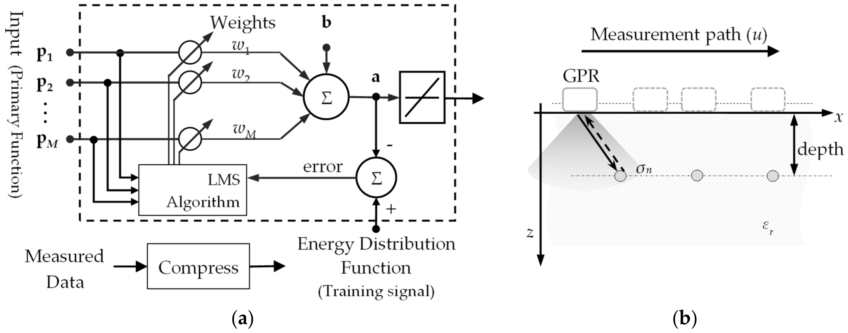
The proposed GPR inversion approach uses an ADALINE [17,18] single layer neural network, as illustrated in Figure 1a. Before training the neural network, the measured GPR data is processed with a data compression procedure (in Section 2.3), to form the energy distribution function that is used as the desired response input (training signal). The input of ADALINE neural network is a series of primary functions extracted from the GPR signal model (also discussed in Section 2.3). Network training is accomplished with the back-propagation algorithm [19,20].
In contrast to the universal neural network, we derived the inversion network from a signal compression procedure, where the measured data is transformed into an energy distribution function. In addition, the proposed network model does not contain the threshold device [17]. We introduce the construction of neural network topology.
2.1. Common-Depth Measurement Model
As shown in Figure 1b, the GPR senses the subsurface zone non-invasively on the surface. For a measurement, a high-frequency electromagnetic pulse is emitted by the transmitting antenna into the subsurface space. Reflections are caused by the targets, and travel back, to be collected by the receiver and recorded as A-scans. By repeating the operation at different positions along the scan path, a B-Scan profile that contains the subsurface information is obtained.
Modeling the subsurface space as a set of dominant scattering centers [21], the received data for the sensor at u can be expressed as:
where σn is the backscattering intensity of nth point target at (xn, zn), and A0 is a coefficient determined by the system configuration. represents the distance between the sensor and the nth point scatter, whereas shows the corresponding two-way travel time. Note that ve is half the real wave velocity that takes the two-way traveling into consideration [16]. Assuming that the GPR works in a lossless or low-loss environment, the dielectric loss η(rn) can be ignored [22]. With this model, it can be seen that the collected echoes are a convolution of the incident wave s(t) with the target’s Green’s function [23].
In this research, we consider a special situation where the targets occur at the same depth, as indicated by the distribution of the target in Figure 1b. Therefore, the unknown parameters for the target are the location xn, and the backscattering intensity σn. In the following, data processing and inversion are all based on this common-depth model.
2.2. Adaptive Linear Element
Adaptive Linear Element (ADALINE) is a single-layer artificial neural network that consists of a weighting vector, a bias and a summation function. One of the advantages of ADALINE neural network is that it can fit any continuous function with an arbitrary level of precision [24].
Assume a special ADALINE neural network, where input and weight can be mapped to the GPR signal and the unknown parameters of the targets, respectively, and the desired response input (training signal) is connected to the observed GPR data; then, by training the network, we are able to invert the targets information, i.e., the horizontal location and backscattering intensity (1).
2.3. Construction of the Neural Network
One of the biggest difficulties in explaining the GPR data is that the exact subsurface medium properties, including dielectric permittivity and conductivity, are usually unavailable [25]. In order to remove the influence of unknown medium, we developed a data compression approach, operated as follows.
For each A-scan trace, Fourier transform is performed along t on (1); then, the received matrix is transformed from spatial-time domain to spatial-frequency domain as
To eliminate the complex phases for data fitting purposes, the energy spectrum is adapted to substitute the space-frequency spectrum, and yields
where Ps(ω) is the power spectrum of the incident signal s(t), and τn,m,u explains the path-difference between nth and mth scatter from the antenna. Note that the second term in (3) reveals the cross modulation effect in GPR measurement.
Next, the incident source wave is removed in (4), yielding a location-varying energy distribution function that relies on the measurement position u and the targets backscattering intensity:
where Es(u) and Ef(u) are
Integrating the ω component in (4) removes the travel time information. In this way we mute the influence of the subsurface medium. Equation (5) indicates that the location-varying energy distribution function contains a stable part Es(u) and a fluctuating part Ef(u). Specifically, Es(u) is a linear combination of a series of quartic function that is defined as the primary function in ADALINE neural network [12], expressed as
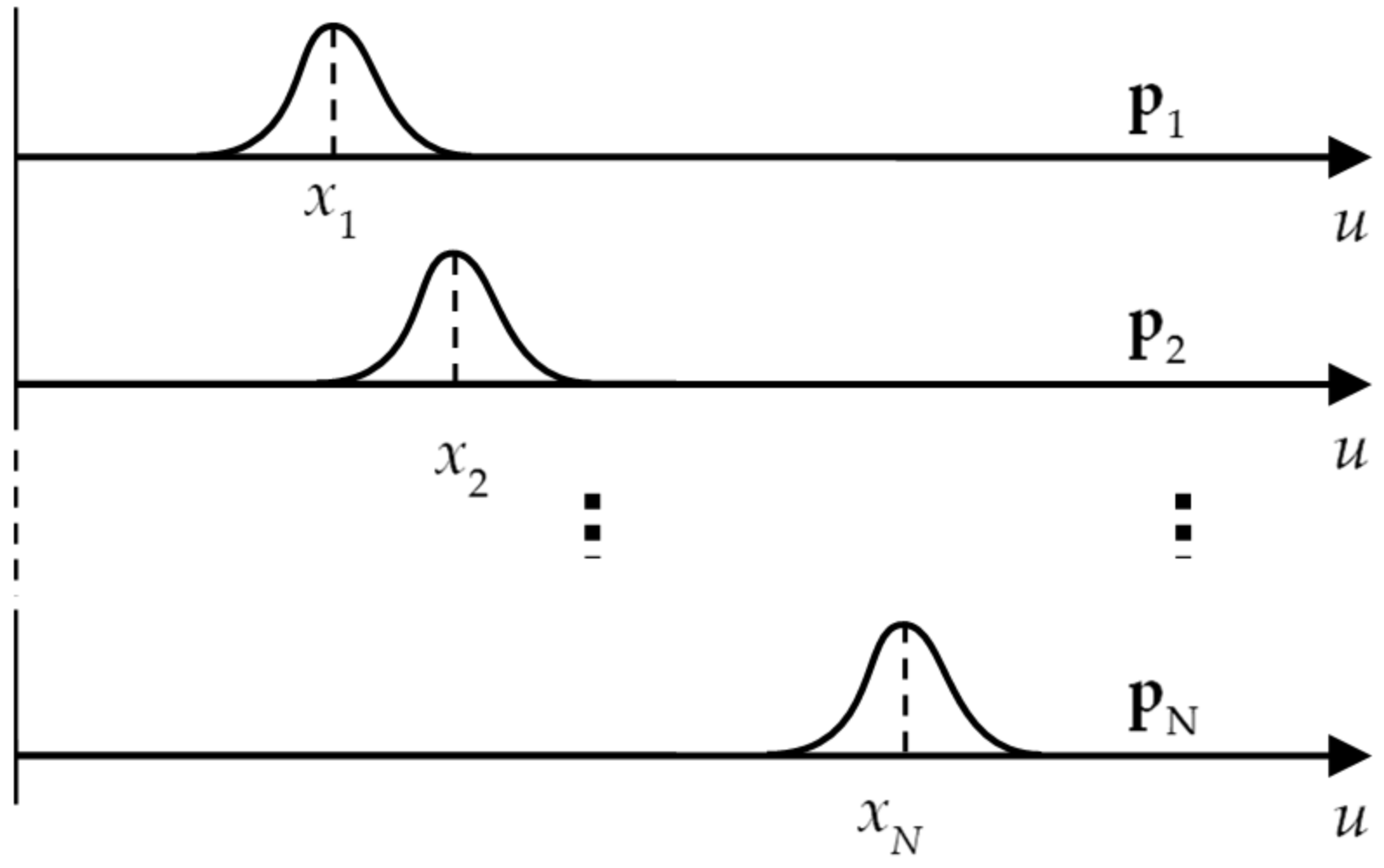
The primary function is centered by the target’s horizontal location xn and has the maximum value . Under the common-depth condition, which means zn = z0 (n = 1, 2, …, N) is a constant, the primary functions differ only by a horizontal shift, as shown in Figure 2. In this way, Es(u) is be a weighted summation of a series of time-shift primary functions, and is independent from the medium properties.
The fluctuating Ef(u) term is a summation of cross modulated sinc function. If only the principal component is analyzed [26], the fluctuating part can be regarded as spatial high-frequency interference, and may be removed using a low pass filter. Thus, the filtered energy distribution function is approximated to:
where the subscript k (k = 1, 2, ..., K) indicates the discrete spatial sampling index. By imposing the following substitution on (7)
and ignoring the constant coefficient, we get:
where
Equation (10) describes a topology of the ADALINE neural network [18], where w is the weight for connections, p is the input, and a is the desired response input (training signal). Mapping the configuration of the ADALINE neural network and training this neural network, the element wk in the weight vector w gives the squared backscattering intensity corresponding to the location uk; in this way, the target’s location and backscattering intensity are obtained.
2.4. Network Configuration
In practical measurements, the targets’ number N in (1) and (10) is not obtained beforehand, which means that the input of the network cannot be determined either. Consider that in the discrete calculation, all the targets occur at discrete positions; if an extra input pm is appended to the network with a zero weight, nothing will change in the output. Assume the real targets’ location set is:
and the input primary functions’ center location set is:
When the following conditions are satisfied,
the network can still fit all the expected output. Increasing of M means an increase in training resources, which implies a relatively small M is necessary. Taking together all considerations, the final network configuration is set as:
To train the target network, the back-propagation algorithm was adopted [20].
3. Results
To enable a precise simulation of GPR data, we used the FDTD tool gprMax [27] to carry out the numerical experiments. A Ricker wavelet with 1 GHz center frequency was set as the incident source for exciting the transmitting antenna, whereas the computational domain covers a 1.0 m × 0.4 m area that was truncated by Perfectly Matched Layer (PML) absorbing boundary condition (ABC). The FDTD grid size was 2.5 mm in both the two dimensions, which means a total of 400 × 160 cells. Concrete with a relative permittivity of 9.0 filled the half-space, in which several point targets were used to simulate the rebar. Two Hertzian dipoles, with an offset of 0.1 m, were employed separately as the transmitting and receiving antenna. All measurements covered a 0.6 m long scan line with trace separation of 1 cm and time window of 10 ns, and were blurred by white Gaussian noise with an SNR of 25 dB. Note that the direct wave is not desired and was canceled with a pre-measured reference background wave in preprocessing. Learning rate for updating the network is 0.02, and in total a maximum iteration of 50,000 was adopted.
3.1. Singular Scatter Scenario
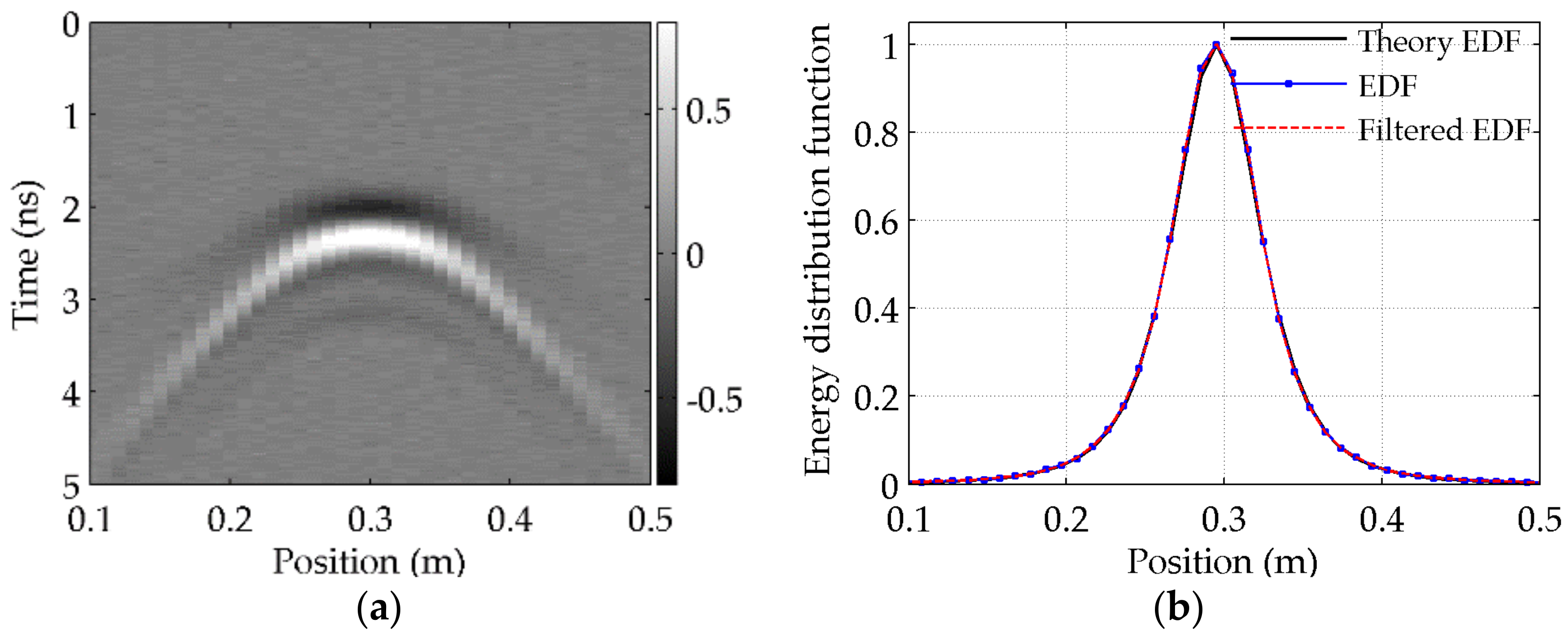
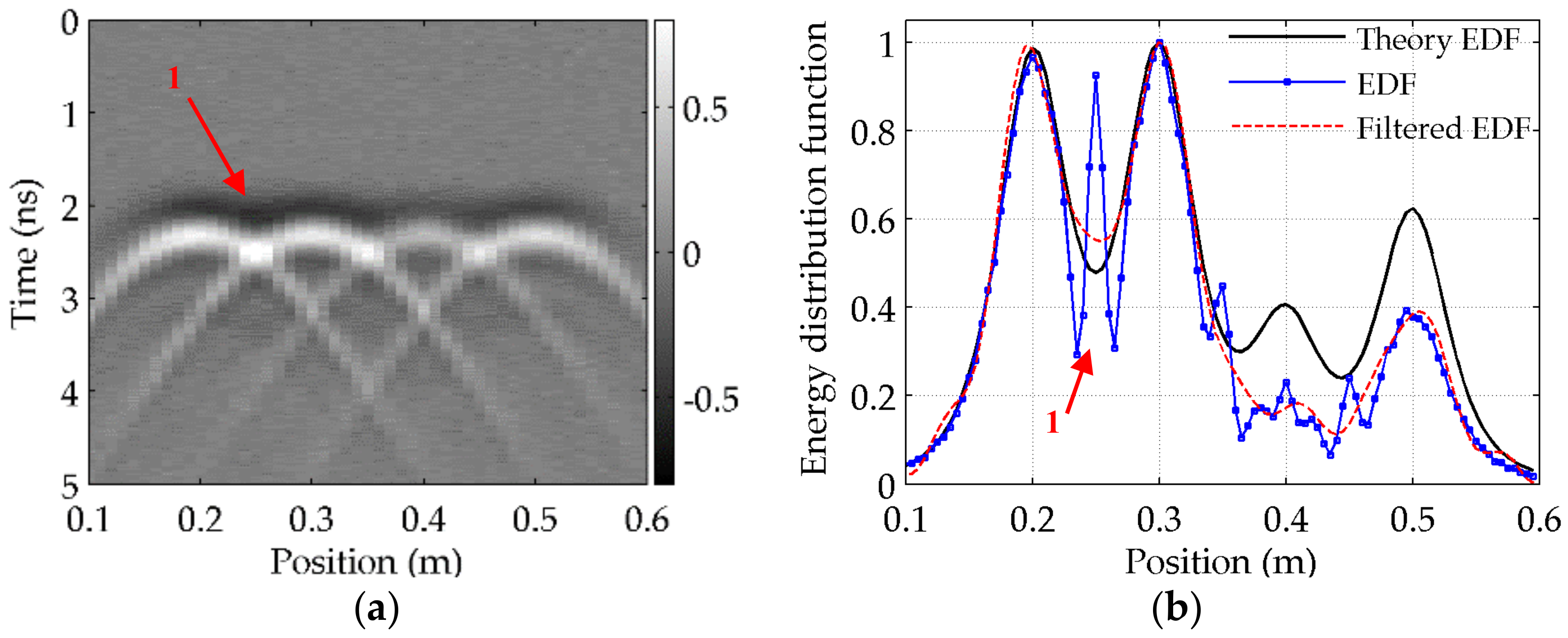
The single scatter biases 0.3 m from the origin, with a depth of 0.05 m and unity backscattering intensity. Figure 3a illustrates the corresponding B-scan data. Note that the direct wave was already removed. The deduced energy distribution function and the filtered spectrum are compared in Figure 3b, with the blue-dot and red-dash line respectively.
Since the cross modulation Ef (5) does not exist for a single target, the obtained energy distribution function (blue-dot line) fits well with the simulation (black line).
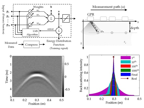
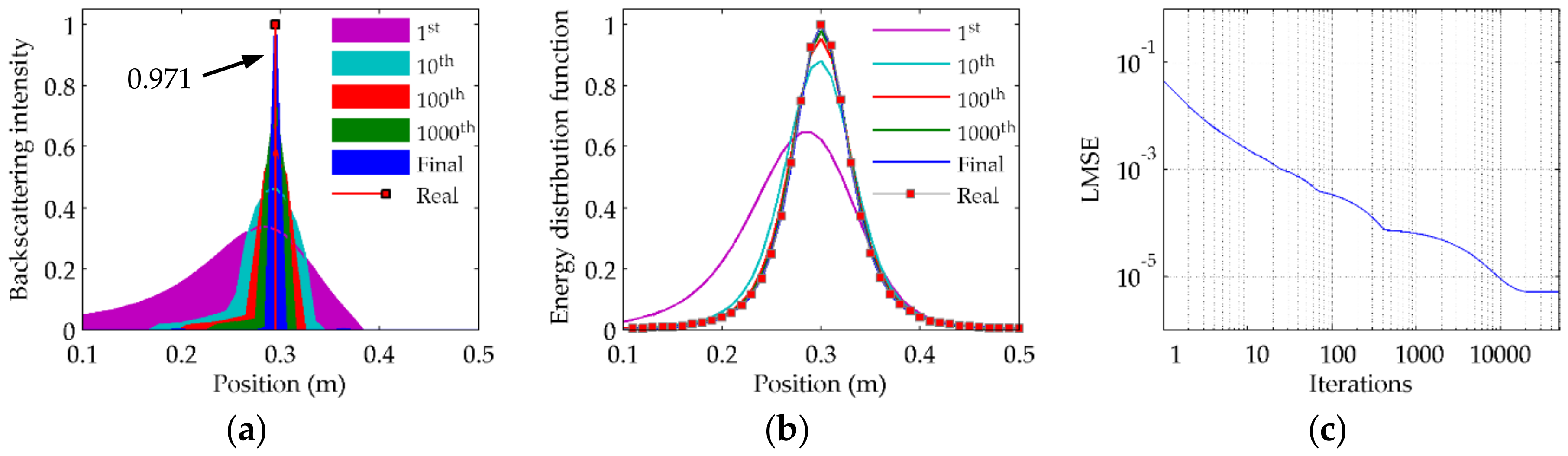
The training of the neural network started with an all zero weight vector, and was accomplished in 84.64 s on a laptop with an Intel 4600 CPU and 8 GB memory, with a fitting least mean square error (LMSE) of 5.14 × 10⁻⁶. Good inversion result can be observed in Figure 4a, which shows that the inverted backscattering intensity converges to 0.3 m, with an impulse of 0.971, that agrees with the preset model (red stem plot). For comparison, the results of the 1st, 10th, 100th, and 1000th iteration are also illustrated, which show a clear evolution history.
The convergence of the inversion can further be verified by the fitted energy distribution function for the 1st, 10th, 100th, and 1000th (Figure 4b). With increasing iterations, the fitted energy distribution function gets closer and closer to the real function, whereas the backscattering intensity concentrates towards the target’s real location. This presents the convergence of the neural network output to the desired response input (training signal). The fast decrease of LMSE (Figure 4c) verifies the efficiency of the inversion.
3.2. Multi Scatters
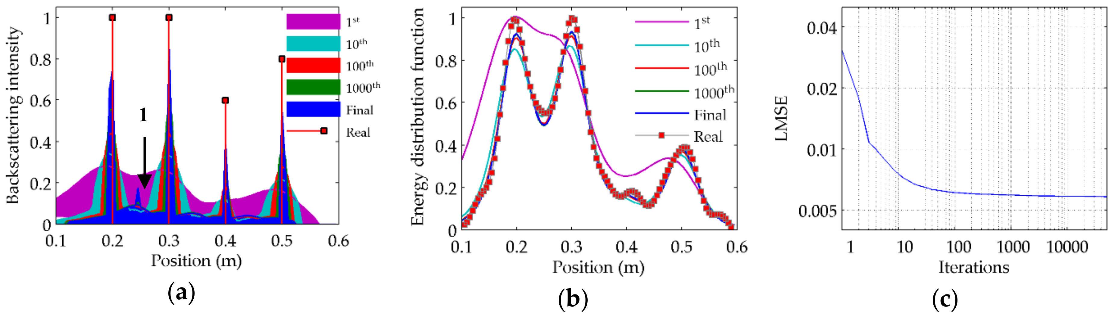
A further experiment with four targets was carried out. These targets, bias 0.2 m, 0.3 m, 0.4 m and 0.5 m from origin with normalized backscattering intensity of 1.0, 1.0, 0.5 and 0.8 respectively, were used to simulate a rebar detection scenario. All the depths are 0.05 m. The corresponding B-scan profile is shown in Figure 5a.
The energy distribution function was calculated, and the network was trained. Figure 5b shows more severe fluctuation in the energy distribution function, caused by the cross modulation effect indicated in (4) and (5). The filtered function shows an apparent weakening compared with the theoretical distribution (red-dash in Figure 5b).
The inversion stopped with the best LMSE (5.8 × 10⁻³). The corresponding results are presented in Figure 6 and Table 1. The inversion result shows a precise estimation of the position, but with more interference between the pulse, and a lower inverted backscattering intensity than expected. The energy diffusion and the cross-modulation lead to the decay of precision for the multi-scatter configuration. Nevertheless, they still keep relative contrast, ensuring that the status of different targets can be compared.
4. Discussion
4.1. Simulation Error
Though the inversion gives a promising result, the simulated result is not exactly the same as the theoretical value. The backscattering intensity, shown in Figure 4a and Figure 6a, indicates the energy from the target diffused to neighbor points and forming side-lobe. This phenomenon cannot be eliminated thoroughly, because of the approximation in the model and derivation, and the limitation of training time. Even though increasing training iteration leads to higher resolution, the computing resources and performance should be balanced.
Another non-negligible problem is the cross modulation indicated by the Ef in (5). The caused inversion error can be observed in Figure 6a at 0.25 m, where a false pulse was inverted. Though the fluctuating part is filtered with a low pass filter, it cannot be thoroughly eliminated, and caused diffusion of signal energy.
4.2. Advantages and Disadvantages of Vertical Information Loss
The transformation from SR(u,w) to EH(u) reduces the space-time joint backscattering intensity distribution to a 1-D energy distribution, which means the depth information and the vertical resolution are both sacrificed. By compressing vertical information, all the objects in the range direction are actually compressed and projected to a backscattering energy distribution. This will harm coherent processing, but will be useful for the application fitting the common-depth model, like rebar detection. The loss of vertical resolution will yield the following benefits:
- The time-space coupling is eliminated.
- Data processing is independent of the medium properties.
- The model can be fitted by the neural network.
Owing to these advantages, vertical compression is helpful to simplify the model, as well as for data interpretation in specific applications.
4.3. Inverting the Depth
In this research, we suppose the depth of the targets is known information, which is not correct. We are now addressing the problem with a multi-layer neural network configuration where the neural network is trained with different primary functions that were derived with various depth values, generating a group of the weight vectors. Then, the combination of weights with minimum LMSEs is determined to be the inversion result; the depth value that leads to the inversion result gives the target depth. Work is ongoing, and shows promising results.
4.4. The Location Precision
As implied by Equations (6)–(8), location precision is determined by the offset between the neighboring imported primary functions, which means, the spatial resolution relies on the number of input elements. When the number of neural network inputs is different to the measurements, spatial resampling on the data is necessary, in order that the data can be mapped to the neural network. For now, we set the neural network to have the same input elements as the number of A-scans; therefore, the location uncertainty is ±Δu/2, where Δu indicates the separation between two A-scans.
4.5. Influence of Medium Heterogeneity
At the current stage, we assumed a uniform concrete environment. In reality, the medium is rather more heterogeneous, and is affected by moisture, porosity, corrosion, etc., meaning that the inversion result would be affected. Since the travel time is compressed in the processing, inversion of the location would not be affected. However, heterogeneity causes additional signal attenuation, as was revealed in the loss of backscattering intensity, resulting in incorrect inversions for the backscattering intensity. One way of overcoming this difficulty might be to use a multi-layer neural network to invert all the measurement zone, but not to limit to the common-depth model. The corresponding work is still being considered, and is expected in the future.
5. Conclusions
Using the neural network to invert the targets’ location and backscattering intensity from GPR data shows the potential to use the neural network as a new inversion strategy for GPR. In contrast to established ways of using a neural network in the remote sensing field, like target detection, recognition, or identification, we accomplish a novel inversion approach based on the data fitting ability of the ADALINE neural network.
This work is based on the common-depth measurement model and an ADALINE neural network. With the dominating point scatter assumption, the observed data is compressed, deriving an energy distribution function and the primary functions. Then, we constructed the ADALINE neural network using the primary functions as input, the energy distribution function as the training signal, and the unknown backscattering intensity as the connection weights. In this way, training the network is equivalent to inverting the target information.
This inversion approach, aiming at solving specific rebar detection and characterization problem, suggests a novel was of using neural network tools for other possible GPR applications. As an early stage study, several problems, such as the depth mismatching, effective training of the neural network, noise influence, and so on, are still in exploration.
Author Contributions
T.L. and Y.S. conceived and designed the theory; T.L., C.H. and Y.S. performed the experiments; T.L. and C.H. analyzed the data; Y.S. contributed analysis tools; T.L. wrote the paper.
Funding
This research was funded by National Natural Science Foundation of China (Grant No. 61372160).
Conflicts of Interest
The authors declare no conflict of interest.
References
- Dérobert, X.; Pajewski, L. TU1208 Open Database of Radargrams: The Dataset of the IFSTTAR Geophysical Test Site. Remote Sens. 2018, 10, 530. [Google Scholar] [CrossRef]
- Dérobert, X.; Iaquinta, J.; Klysz, G.; Balayssac, J. Use of capacitive and GPR techniques for the non-destructive evaluation of cover concrete. NDT&E Int. 2008, 41, 44–52. [Google Scholar]
- Kaur, P.; Dana, K.J.; Romero, F.A.; Gucunski, N. Automated GPR Rebar Analysis for Robotic Bridge Deck Evaluation. IEEE Trans. Cybern. 2016, 46, 2265–2276. [Google Scholar] [CrossRef] [PubMed]
- Evans, R.D.; Frost, M.W.; Stonecliffe-Jones, M.; Dixon, N. Ground-penetrating radar investigations for urban roads. Proc. Inst. Civ. Eng. 2006, 159, 105–111. [Google Scholar] [CrossRef] [Green Version]
- Gamba, P.; Lossani, S. Neural detection of pipe signatures in ground penetrating radar images. IEEE Trans. Geosci. Remote Sens. 2000, 38, 790–797. [Google Scholar] [CrossRef]
- Shaw, M.R.; Millard, S.G.; Molyneaux, T.C.K.; Taylor, M.J.; Bungey, J.H. Location of steel reinforcement in concrete using ground penetrating radar and neural networks. NDT&E Int. 2005, 38, 203–212. [Google Scholar]
- Caorsi, S.; Cevini, G. An electromagnetic approach based on neural networks for the GPR investigation of buried cylinders. IEEE Trans. Geosci. Remote Sens. 2005, 2, 3–7. [Google Scholar] [CrossRef]
- Travassos, X.L.; Vieira, D.A.G.; Ida, N.; Vollaire, C.; Nicolas, A. Characterization of Inclusions in a Nonhomogeneous GPR Problem by Artificial Neural Networks. IEEE Trans. Magn. 2008, 44, 1630–1633. [Google Scholar] [CrossRef]
- Sbartaï, Z.M.; Laurens, S.; Viriyametanont, K.; Balayssac, J.P.; Arliguie, G. Non-destructive evaluation of concrete physical condition using radar and artificial neural networks. Constr. Build. Mater. 2009, 23, 837–845. [Google Scholar] [CrossRef]
- Núñez-Nieto, X.; Solla, M.; Gómez-Pérez, P.; Lorenzo, H. GPR Signal Characterization for Automated Landmine and UXO Detection Based on Machine Learning Techniques. Remote Sens. 2014, 6, 9729–9748. [Google Scholar] [CrossRef]
- Lameri, S.; Lombardi, F.; Bestagini, P.; Lualdi, M.; Tubaro, S. Landmine detection from GPR data using convolutional neural networks. In Proceedings of the 25th European Signal Processing Conference (EUSIPCO), Kos, Greece, 28 August 2017–2 September 2017; pp. 508–512. [Google Scholar]
- Frieß, T.; Harrison, R.F. A kernel-based Adaline for function approximation. Intell. Data Anal. 1999, 3, 307–313. [Google Scholar] [CrossRef]
- Li, M.; Huang, C.; Su, Y. A Method of Removing Interference Fringes on Spherical Subsurface Imaging with Continuous Wave Penetrating Radar. In Proceedings of the 2016 16th International Conference on Ground Penetrating Radar (GPR), Hong Kong, China, 13–16 June 2016; pp. 1–4. [Google Scholar]
- Huang, C.; Liu, T.; Lu, M.; Su, Y. Holographic Subsurface Imaging for Medical Detection. In Proceedings of the 2016 16th International Conference on Ground Penetrating Radar (GPR), Brussels, Belgium, 30 June–4 July 2014. [Google Scholar]
- Song, X.; Su, Y.; Zhu, Y.; Huang, C.; Lu, M. Improving Holographic Radar Imaging Resolution via Deconvolution. In Proceedings of the 2016 16th International Conference on Ground Penetrating Radar (GPR), Brussels, Belgium, 30 June–4 July 2014; pp. 633–636. [Google Scholar]
- Zhu, S.; Huang, C.; Su, Y.; Sato, M. 3D Ground Penetrating Radar to Detect Tree Roots and Estimate Root Biomass in the Field. Remote Sens. 2014, 6, 5754–5773. [Google Scholar] [CrossRef]
- Widrow, B.; Lehr, M.A. 30 years of adaptive neural networks: Perceptron, Madaline, and backpropagation. Proc. IEEE 1990, 78, 1415–1442. [Google Scholar] [CrossRef]
- Rojas, R. Neural Networks—A Systematic Introduction; Springer-Verlag New York, Inc.: New York, NY, USA, 1996. [Google Scholar]
- Chauvin, Y. A Back-Propagation Algorithm with Optimal Use of Hidden Units; Morgan Kaufmann Publishers Inc.: San Mateo, CA, USA, 1989; pp. 519–526. [Google Scholar]
- Sarkar, D. Methods to Speed Up Error Back-Propagation Learning Algorithm; ACM: New York, NY, USA, 1995; pp. 519–544. [Google Scholar]
- Langman, A. The Design of Hardware and Signal Processing for a Stepped Frequency Continuous Wave Ground Penetrating Radar. Ph. D. Thesis, University of Cape Town, Cape Town, South Africa, 2002. [Google Scholar]
- Jol, H.M. Ground Penetrating Radar Theory and Applications; Elsevier Science: New York, NY, USA, 2009; pp. 595–604. [Google Scholar]
- Su, Y.; Huang, C.; Lei, W. Ground Penetrating Radar—Theory and Applications; Science Press: Beijing, China, 2006. [Google Scholar]
- Wu, J.; Lin, Z.; Hsu, P. Function approximation using generalized adalines. IEEE Trans. Neural Netw. 2006, 17, 541–558. [Google Scholar] [PubMed]
- Busch, S.; van der Kruk, J.; Vereecken, H. Improved Characterization of Fine-Texture Soils Using on-Ground GPR Full-Waveform Inversion. IEEE Trans. Geosci. Remote Sens. 2014, 52, 3947–3958. [Google Scholar] [CrossRef]
- Cumming, I.G.; Wong, F.H. Digital Processing of Synthetic Aperture Radar Data: Algorithms and Implementation; Artech House Print on Demand: Norwood, MA, USA, 2005; pp. 168–175. [Google Scholar]
- Warren, C.; Giannopoulos, A.; Giannakis, I. gprMax: Open source software to simulate electromagnetic wave propagation for Ground Penetrating Radar. Comput. Phys. Commun. 2016, 209, 163–170. [Google Scholar] [CrossRef]
Figure 1.
(a) Diagram of the neural network based GPR data inversion approach. (b) Common-offset and common-depth measurement model. The targets distribute at a same depth.
Figure 1.
(a) Diagram of the neural network based GPR data inversion approach. (b) Common-offset and common-depth measurement model. The targets distribute at a same depth.

Figure 2.
The primary function sets.

Figure 3.
Numerical experimental data with a single scatter. (a) presents the radargram of the target. Note that the direct wave is canceled with a pre-measured reference background signal. (b) shows the energy distribution function derived from (a), where the direct obtained and filtered energy distribution function (EDF) are illustrated with blue-dot and red-dash lines respectively. For comparison, the black line presents the theoretical value.

Figure 4.
Inversion result for the single scatter scenario. (a) presents the distribution of the inverted backscattering intensity during the network training. The results of the 1st, 10th, 100th, 1000th and final iterations are illustrated with different colors (see the legend). Since the initial set is all zeros, it is not visible in the figure. (b) shows the fitted energy distribution function. (c) gives the evolution of LMSE during the network training, i.e., inversion. Note that both the x- and y-axis are displayed with a logarithmic scale.

Figure 5.
Numerical experimental data with multi scatters. (a) The radargram of the four preset targets biases 0.2 m, 0.3 m, 0.4 m and 0.5 m from the origin, with normalized backscattering intensities of 1.0, 1.0, 0.6 and 0.8 respectively. All depths are 0.05 m. Note that the direct wave is canceled with a pre-measured reference background signal. (b) shows the energy distribution function derived from (a), where the direct obtained and filtered energy distribution functions are illustrated with blue-dot and red-dash lines. For comparison, the black line presents the theoretical value. In (a,b), the red arrow indicates the strong interference of two echos, showing the cross modulation effect between targets.

Figure 6.
Inversion result for the multi-scatter scenario. (a) presents the distribution of the inverted backscattering intensity during the network training. The results of the 1st, 10th, 100th, 1000th and final iterations are illustrated with different colors (see the legend). Since the initial set is all zeros, it is not visible in the figure. A false pulse appears at 0.25 m, and is indicated with number 1, corresponding to Figure 5. (b) shows the evolution of the fitted energy distribution function. (c) gives the evolution of LMSE in the network training, i.e., inversion..


Table 1.
Inversion of the multi-target experiment.
| No. | Target Location | Preset Backscattering Intensity | Inverted Backscattering Intensity |
|---|---|---|---|
| 1 | 0.2 m | 1.00 | 0.747 |
| 2 | 0.3 m | 1.00 | 0.847 |
| 3 | 0.4 m | 0.60 | 0.386 |
| 4 | 0.5 m | 0.80 | 0.469 |
© 2018 by the authors. Licensee MDPI, Basel, Switzerland. This article is an open access article distributed under the terms and conditions of the Creative Commons Attribution (CC BY) license (http://creativecommons.org/licenses/by/4.0/).
Share and Cite
MDPI and ACS Style
Liu, T.; Su, Y.; Huang, C. Inversion of Ground Penetrating Radar Data Based on Neural Networks. Remote Sens. 2018, 10, 730. https://doi.org/10.3390/rs10050730
AMA Style
Liu T, Su Y, Huang C. Inversion of Ground Penetrating Radar Data Based on Neural Networks. Remote Sensing. 2018; 10(5):730. https://doi.org/10.3390/rs10050730
Chicago/Turabian StyleLiu, Tao, Yi Su, and Chunlin Huang. 2018. "Inversion of Ground Penetrating Radar Data Based on Neural Networks" Remote Sensing 10, no. 5: 730. https://doi.org/10.3390/rs10050730
Note that from the first issue of 2016, this journal uses article numbers instead of page numbers. See further details here.