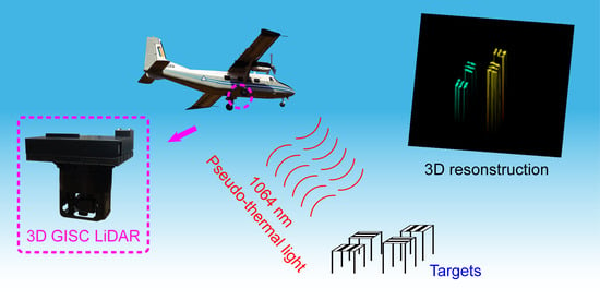
Airborne Near Infrared Three-Dimensional Ghost Imaging LiDAR via Sparsity Constraint

Abstract

Three-dimensional ghost imaging LiDAR via sparsity constraint (3D GISC LiDAR), as a staring imaging method, can obtain both the range information and spatial distribution of a remote target with a single-pixel time-resolved detector. However, previous demonstrations mainly focused on the relatively static scene in visible light. Here we propose an airborne near infrared 3D GISC LiDAR system and airborne high-resolution imaging is implemented. Experimental results show that an image with 0.48 m horizontal resolution as well as 0.5 m range resolution at approximately 1.04 km height can be achieved. Some considerations on the improvement of this LiDAR system are also discussed.

1. Introduction

Three-dimensional (3D) imaging can provide literal imagery easily interpreted at ranges beyond what passive two-dimensional (2D) monochromatic imaging can provide [1]. In many fields such as earth mapping, environmental monitoring and autonomous driving, 3D imaging LiDAR which is based on the mechanism of time-of-flight (TOF) measurement proves an effective strategy and has been applied successfully for many years [1,2,3]. Because the near infrared (NIR) light is much safer for human eyes, suffers less influence from background radiation, and has better penetrability in real atmosphere, NIR 3D imaging LiDAR technique is becoming a new tendency nowadays [4,5]. Although NIR scanning imaging LiDAR can obtain 3D imagery with a time-resolved single-pixel detector, it takes a long time to scan the interested area so that this LiDAR is difficult to image a high-speed moving target [1]. NIR non-scanning imaging LiDAR, as a staring imaging method, can cover the whole area of the target and obtain the target’s 3D image in a single exposure [1]. However, its detection sensitivity is low; and time-resolved detectors with large array of pixels are expensive and hard to manufacture. Therefore, new staring NIR 3D imaging methods are urgently required. 3D ghost imaging via sparsity constraint (3D GISC) is a novel 3D imaging mechanism which combines ghost imaging approach with compressive sensing technique [6,7,8]. With only one time-resolved single-pixel detector, this method can obtain high-resolution 3D imagery by using measurements below the Nyquist limit [9,10,11]. This brand-new technique is also a staring imaging mechanism and has the capability of both high efficiency in information extraction and high sensitivity in signal detection, which is developing into a new 3D imaging LiDAR [9,10,11,12,13,14,15,16]. In 2012, our group invented a 2D GISC LiDAR system at 532 nm wavelength and high-resolution 2D imaging was experimentally demonstrated [10]. Later, when the TOF technique was used to measure the target’s reflection signals and structured compressive sensing reconstruction algorithm was adopted to 3D reconstruction, we had also obtained 3D imagery of a scene at a range of approximately 1.0 km [11,12]. In those previous experimental demonstrations both the LiDAR system and the target were static [10,11,12,13]. However, in remote sensing applications such as airborne platform, vehicle platform, and moving targets with high speed, there usually exists relative movement between the LiDAR system and the target, while GISC LiDAR usually requires lots of measurements to achieve the information of interested target, which consumes a long acquisition time. Hence the relative motion between the LiDAR system and the target during the sampling process will result in motion blur inevitably [17,18,19]. Although some algorithms or strategies can overcome the motion blur to some extent [18,19], it still does not satisfy the application requirements of airborne remote sensing. Therefore, for the system of airborne 3D GISC LiDAR, some motion compensation technique should be applied to stare at the same scene during the sampling process.

2. Materials and Methods

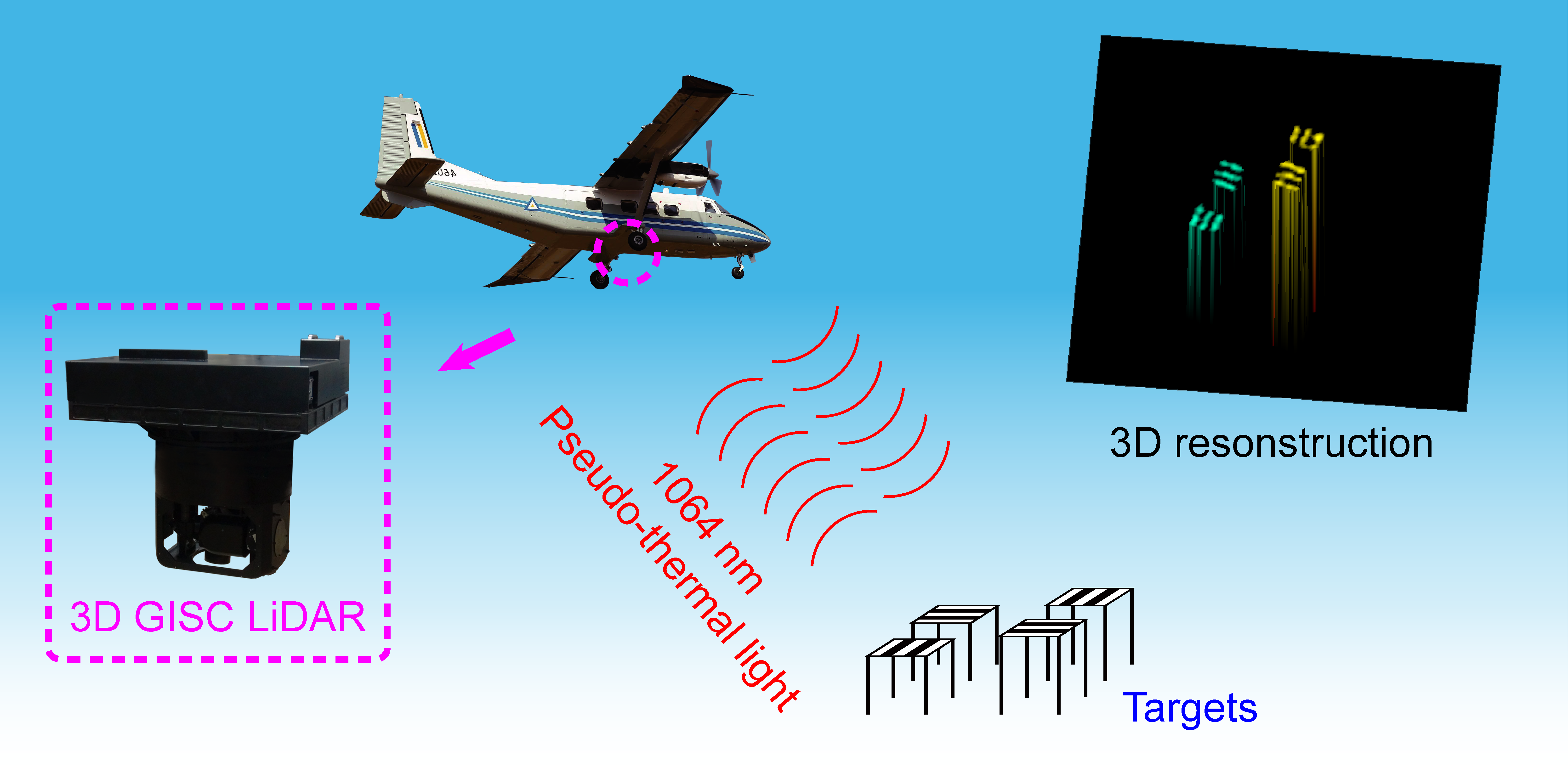
2.1. System Design

Figure 1a provides a photo and the mounting diagram of the proposed airborne NIR 3D GISC LiDAR system and Figure 1b,c present the principle schematic. The LiDAR’s main body is firstly mounted on a stabilized platform and then mounted on the airframe via a support frame. This LiDAR system mainly consists of a static NIR 3D GISC LiDAR subsystem (Figure 1a), which is similar to the system described in Ref. [11]) and a motion compensation subsystem (MCS, Figure 1b). For the static LiDAR subsystem, the pseudo-thermal light source, which mainly consists of a center-wavelength $\lambda$ = 1064 nm solid-state pulsed laser with about 6 ns pulse width at a repetition rate of 2 kHz and a rotating diffuser, generates random speckle patterns at the stop. The laser’s spot diameter illuminating on the rotating diffuser is D = 0.9 mm and the distance between the diffuser and the stop is 59.2 mm. The diffuser is a ground glass disk controlled by a high-precision motor and its rotating speed is 60 r/min. The light emitted from the source is then divided by a beam splitter (BS1) into a reference and an object paths. In the reference path, a charge-coupled device (CCD) is placed on the image plane of the speckle pattern at the stop and the magnification of imaging system is 1×. In the experiment, we have used a Mikrotron CAMMC1362 EoSen mono high-speed CCD camera whose pixel size is 14 $\mathsf{\mu }$m × 14 $\mathsf{\mu }$m. The camera’s frame frequency is 2 kHz and the exposure time is set as 0.1 ms. In the object path, the speckle patterns at the stop are imaged, reflected by a tracking mirror, onto the target by the emitting objective lens $f_0$ = 180.25 mm. The effective transmission aperture of the objective lens is about 5.57 mm which corresponds to a diffraction limit of 0.24 m at 1.04 km, while the horizontal resolution on the target’s planar is about 0.4 m limited by the speckle’s transverse size at the stop [20,21]. The photons reflected from the target are firstly reflected by the same tracking mirror, collected by a receiving lens $f_2$ and then divided by another beam splitter (BS2). For the transmission path, only the 1064 nm photons pass through an interference filter with the center wavelength at 1064 nm and 1 nm half-bandwidth into a photomultiplier tube (PMT) connected with an amplifier (FEMTO HCA-200M-20K-C) and a high-speed digitizer of 1 G/s (which is equivalent to a time-resolved single-pixel bucket detector). The bandwidth of the amplifier is 200 MHz, and the transmission aperture of receiving lens is 55 mm and its focal length is 296.5 mm. Note that limited by the PMT’s numerical aperture and active size, the effective transmission aperture of receiving lens is only 19 mm according to the theorem of Lagrange invariant [22]. The circular field of view (FOV) on the target plane for both the emitting and receiving system is about 58 m/1040 m. For the reflection path, the 420 nm∼620 nm photons reflected from the target are imaged onto the monitor CCD camera whose performance is the same as the reference CCD camera.

In the MCS, a two-levels compensation mechanism based on inertial navigation and opto-electronic detection technique [23,24] is designed. The first level of MCS mainly consists of a global positioning system (GPS), an inertial measurement unit (IMU), and a Leica PAV80 stabilized platform, which is used to reduce the influence of the aircraft’s posture variation on the LiDAR’s posture. Then both the LiDAR’s residual posture variation and the relative movement between the target and the aircraft are compensated by the second level of MCS. For our LiDAR system, the second level of MCS has two working modes. One is controlling the tracking mirror based on the GPS information of both the aircraft and the target and the IMU information of the LiDAR system. Limited by the precision of GPS and IMU, the pointing accuracy can only reach 1.7 mrad@10s (RMS). The other is controlling the tracking mirror based on the traditional opto-electronic detection technique, according to the high-resolution image recorded by the monitor CCD camera. In this case, our LiDAR system’s pointing accuracy can reach 0.1 mrad@10s (RMS). In addition, the tracking mirror used in our LiDAR system can provide an observation scope with −20${}^{\circ }$∼+44${}^{\circ }$ and the FOV recorded by the monitor CCD camera is about 29 m/1040 m.

2.2. Structured 3D GISC Reconstruction

In the target’s 3D information reconstruction, the structured 3D GISC method [12] is adopted by this airborne NIR 3D GISC LiDAR. The speckle intensity distribution ($m\times n$ pixels) recorded by the reference camera shown in Figure 1b in each measurement can be reshaped into a row vector of length N (N = $m\times n$) to form a single row of the measurement matrix denoted by A. Then the TOF signal recorded by the single-pixel time-resolved detector in each measurement is used to form a Q length row of the signal matrix denoted by Y. After M measurements ($M\ll N$), the $M\times N$ measurement matrix A and the $M\times Q$ signal matrix Y can be obtained. If we use a column vector ${\widehat{x}}_i$ of length N to represent the unknown 3D target at each TOF bin, there will exists a simple relationship between the reflection signals and the 3D target [12],

$$Y=AX+E$$

(1)

where $X=\left[{\widehat{x}}_1,\dots ,{\widehat{x}}_i,\dots {\widehat{x}}_Q\right]$, and E denote the noise exists in Y.

For 3D GISC reconstruction, taking the orthogonal property caused by target’s occlusion into consideration, the structured 3D GISC reconstruction can be expressed as [11,12],

$$X=\left[{\widehat{x}}_1,\dots ,{\widehat{x}}_i,\dots {\widehat{x}}_Q\right]=argmin\frac{1}{2}{∥{\widehat{y}}_i-A{\widehat{x}}_i∥}_2^2+{\tau }_i{∥{\widehat{\theta }}_i∥}_1^2+{\tau }_c\mu \left(\widehat{X}\right)$$

(2)

where ${\tau }_i$ and ${\tau }_c$ are constants, ${∥\dots ∥}_1$, and ${∥\dots ∥}_2$ denotes the 1-norm and 2-norm respectively, ${\widehat{x}}_i=\mathsf{\Psi }{\widehat{\theta }}_i$, $\mathsf{\Psi }$ is the transform operator to the sparse representation basis, and $\mu \left(\widehat{X}\right)$ is the average value of absolute inner products between any of two columns of $\widehat{X}$ [12]. By solving this typical convex optimization problem, we can obtain the 3D GISC reconstruction of the target after a simple transformation of $z=\frac{TOF\times c}{2}$, c denotes the light speed.

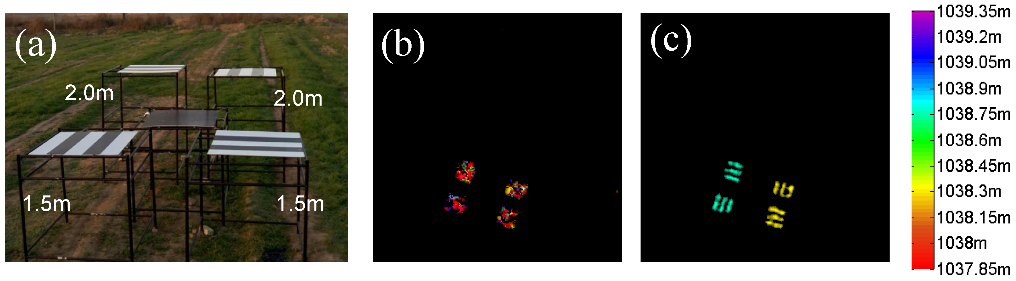
2.3. Experimental Section

To verify the performance of this airborne NIR 3D GISC LiDAR system, we performed experiments by using a Y-12 aircraft in Xi’an, China. The aircraft’s flight altitude was about 1.04 km and the flying speed was approximately 208 km/h. As schematically depicted in Figure 2a, when the aircraft is flying over the position 1, the MCS will guide the LiDAR system towards the target’s general area according to the real-time GPS and IMU information (the GPS and IMU information of this LiDAR system is measured in real-time whereas the target’s GPS information is measured before the experiment). Secondly, when the target enters into the FOV of the monitor CCD camera (namely the position 2 as displayed in Figure 2a), the traditional opto-electronic detection technique starts and provides high resolution tracking and pointing. Afterwards, when the aircraft is flying over the position 3 of Figure 2a, the sampling process will begin and last for a short period of time to obtain enough measurements (the positions 3∼6 in Figure 2a). It was worth mentioning that in the flight process, the distance between the LiDAR system and the target, as illustrated in Figure 2b,c, was always changed because of the aircraft’s movement, which would lead to the blur of horizontal resolution and range resolution for 3D GISC LiDAR. However, the blur of range resolution could be corrected by proper pre-processing of the TOF signals and the technique demonstrated in Ref. [19] could be adopted for the blur of horizontal resolution.

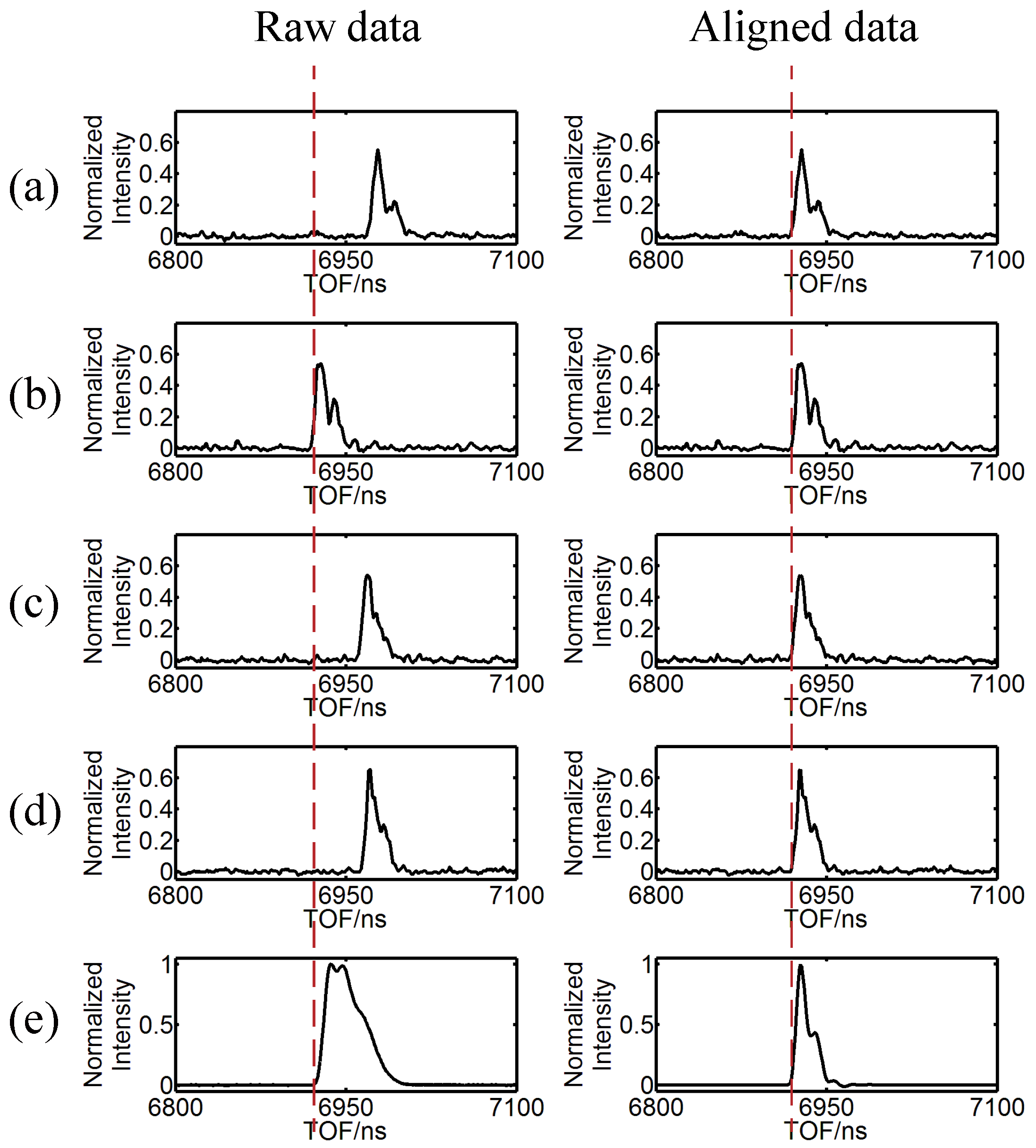
2.4. Pre-Processing of the TOF Signals

One obstacle in successful 3D reconstruction is that because the aircraft is constantly flying during the sampling process, the relative range from the LiDAR system to the target changes all the time. Therefore, as shown in Figure 2b,c, the TOF signals of the target at different range will be mixed together, which will result in 3D reconstruction failure. Here we propose a simple pre-processing of the TOF signals as follows. Firstly, a maximum normalization for all reflection signals is performed. Then the 0.1 threshold position of every reflection signal is treated as the site of rinsing edge. Finally, we align all signals’ rising edges with a fixed reference position (without loss of generality, the nearest point, 4 in Figure 2b is reasonable). This TOF signals’ pre-processing is schematically depicted in the following Figure 3 in details. Clearly, after applying this simple pre-processing, all TOF signals during the sampling can have the same reference position, which can be used in the 3D GISC reconstruction algorithm described above [12].

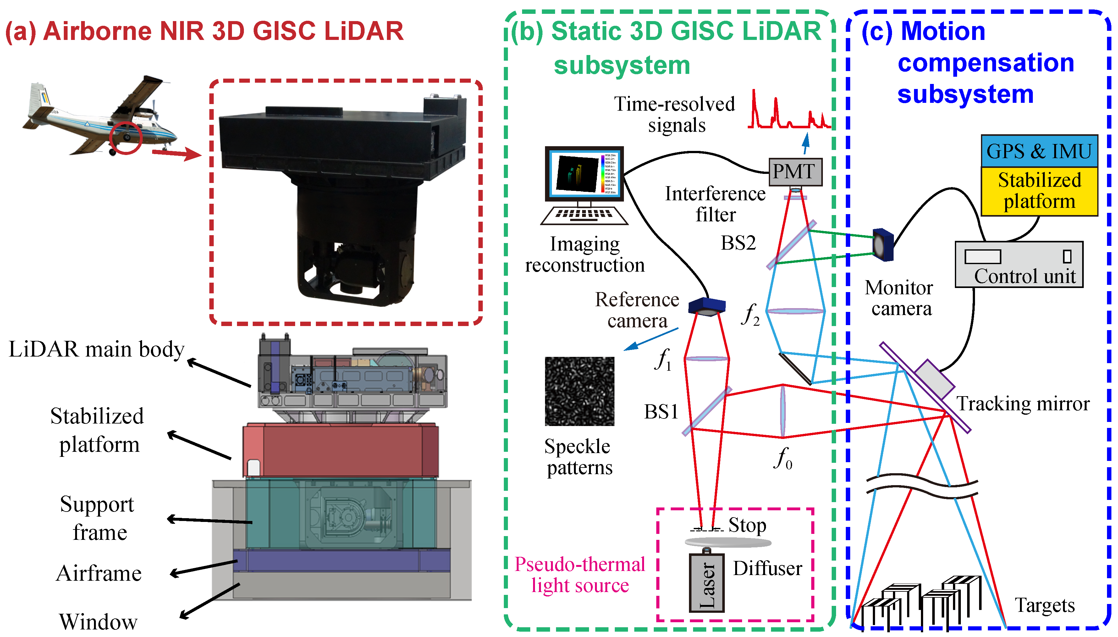
3. Results and Discussion

In the experimental demonstration, a set of three-string plates with center-to-center separation of 0.48 m and height difference of 0.5 m (Figure 4a) were used to test the LiDAR’s 3D imaging capability. The area of the reference camera shown in Figure 1b was set as 220 × 220 pixels. The measurements used for 3D reconstruction was 8000 and the effective sampling time was 4 s. Therefore, the angle $\theta$ shown in Figure 2a was approximately 12.7${}^{\circ }$ and the maximum range variation was 6.4 m when the flight altitude on the position 4 was about 1.04 km. On the basis of the theory described in Ref. [19], in this case the maximum motion blur caused by axial range variation was 0.18 m, which could be negligible in contrast with the LiDAR system’s designed horizontal resolution 0.4 m. Therefore, the axial range variation during the sampling time did not influence the horizontal resolution of 3D images. For the 3D image reconstruction, the algorithm described in Section 2.2 and the discrete cosine transformation were adopted [11,12]. In addition, the reconstructed image at each TOF bin has been post-processed (the value of image, below 20% of the peak intensity, was set as 0). As discussed above, the target’s TOF changed all the time in the flight process. So without any pre-processing, the TOF signals at difference range would be mixed together, which resulted in the degradation of range resolution and the failure of 3D reconstruction (Figure 4b). By applying the TOF signals’ pre-processing technique described in Section 2.4 before image reconstruction, the 3D GISC reconstruction result was depicted in Figure 4c. Obviously, the target can be resolved in both the horizontal and range directions, which suggests that the airborne NIR 3D GISC LiDAR experimental demonstration has been implemented successfully.

This proposed 3D LiDAR system based on a static GISC LiDAR and a MCS still exists some problems. First of all, when the effective transmission aperture of the emitting objective lens is large enough, the final horizontal resolution of this LiDAR system is mainly restricted by the accuracy of motion compensation. Secondly, the opto-electronic technique utilized in MCS will be disabled in the cases such as at night or a low visibility weather. Therefore, some operating modes like push-broom scanning in which the MCS can be discarded may be better. Thirdly, compared to the previous static 3D GISC LiDAR system reported in Ref. [11], the reconstruction quality is degraded because the numerical aperture of the receiving system is not large enough to provide a high detection signal-to-noise ratio (a detailed analysis will be reported in the other journal) and multiple-input approaches may be adopted in the next work [25]. Fourthly, in order to reduce the influence of the backscattering of light field on the detection signal-to-noise ratio, a bistatic optical structure is utilized in present LiDAR system, which is difficult to expand to high-resolution telescope with a large aperture because such two telescopes should be used. Therefore, the integrated receiving and emitting optical scheme will be a development tendency for 3D GISC LiDAR. Finally, in contrast with traditional passive imaging, 3D GISC LiDAR has lost the abundant texture characteristic of scenes, thus the combination of 3D GISC LiDAR with passive imaging will be a new direction in the field of earth mapping.

4. Conclusions

In summary, we have developed an airborne NIR 3D GISC LiDAR system by combining a static 3D GISC LiDAR with a two-levels motion compensation mechanism. Borne on a Y-12 aircraft, we experimentally verified that the system had the capability of motion deblurring, and 3D imaging with 0.48 m horizontal resolution as well as 0.5 m range resolution at approximately 1.04 km height was demonstrated. However, for practical application of this 3D GISC LiDAR system, the improvement of motion compensation accuracy, further optimization of optical structure and the combination with passive imaging may be a research focus in the next work. When both the range resolution and imaging speed are further improved, this 3D GISC technique can be applied to automatic driving, 3D non-invasive biological imaging and so on.

References

1. Council, N.R. (Ed.) Laser Radar: Progress and Opportunities in Active Electro-Optical Sensing, 1st ed.; National Academies Press: New York, NY, USA, 2014; pp. 6–106. [Google Scholar]
2. Mallet, C.; Bretar, F. Full-waveform topographic lidar: State-of-the-art. ISPRS J. Photogramm. Remote Sens. 2009, 64, 1–16. [Google Scholar] [CrossRef]
3. Geiger, A.; Lenz, P.; Urtasun, R. Are we ready for autonomous driving? The KITTI vision benchmark suite. In Proceedings of the 2012 IEEE Conference on Computer Vision and Pattern Recognition (CVPR), Providence, RI, USA, 16–21 June 2012; IEEE: Piscataway, NJ, USA, 2012; pp. 3354–3361. [Google Scholar]
4. Kambezidis, H.D.; Djepa-Petrova, V.; Adamopoulos, A.D. Radiative transfer. I. Atmospheric transmission monitoring with modeling and ground-based multispectral measurements. Appl. Opt. 1997, 36, 6976–6982. [Google Scholar] [CrossRef] [PubMed]
5. Itzler, M.A.; Entwistle, M.; Wilton, S.; Kudryashov, I.; Kotelnikov, J.; Jiang, X.; Piccione, B.; Owens, M.; Rangwala, S. Geiger-Mode LiDAR: From Airborne Platforms To Driverless Cars. In Proceedings of the Applied Industrial Optics: Spectroscopy, Imaging and Metrology, San Francisco, CA, USA, 26–29 June 2017; Optical Society of America: Washington, DC, USA, 2017; p. ATu3A.3. [Google Scholar]
6. Donoho, D.L. Compressed sensing. IEEE Trans. Inf. Theory 2006, 52, 1289–1306. [Google Scholar] [CrossRef]
7. Candès, E.J.; Wakin, M.B. An introduction to compressive sampling. IEEE Signal Process. Mag. 2008, 25, 21–30. [Google Scholar] [CrossRef]
8. Katz, O.; Bromberg, Y.; Silberberg, Y. Compressive ghost imaging. Appl. Phys. Lett. 2009, 95, 131110. [Google Scholar] [CrossRef]
9. Zhang, Y.; Edgar, M.P.; Sun, B.; Radwell, N.; Gibson, G.M.; Padgett, M.J. 3D single-pixel video. J. Opt. 2016, 18, 035203. [Google Scholar] [CrossRef]
10. Zhao, C.; Gong, W.; Chen, M.; Li, E.; Wang, H.; Xu, W.; Han, S. Ghost imaging lidar via sparsity constraints. Appl. Phys. Lett. 2012, 101, 141123. [Google Scholar] [CrossRef]
11. Gong, W.; Zhao, C.; Yu, H.; Chen, M.; Xu, W.; Han, S. Three-dimensional ghost imaging lidar via sparsity constraint. Sci. Rep. 2016, 6, 26133. [Google Scholar] [CrossRef] [PubMed]
12. Yu, H.; Li, E.; Gong, W.; Han, S. Structured image reconstruction for three-dimensional ghost imaging lidar. Opt. Express 2015, 23, 14541–14551. [Google Scholar] [CrossRef] [PubMed]
13. Sun, M.; Edgar, M.P.; Gibson, G.M.; Sun, B.; Radwell, N.; Lamb, R.; Padgett, M.J. Single-pixel three-dimensional imaging with time-based depth resolution. Nat. Commun. 2016, 7, 12010. [Google Scholar] [CrossRef] [PubMed]
14. Hardy, N.D.; Shapiro, J.H. Computational ghost imaging versus imaging laser radar for three-dimensional imaging. Phys. Rev. A 2013, 87, 023820. [Google Scholar] [CrossRef]
15. Erkmen, B.I. Computational ghost imaging for remote sensing. JOSA A 2012, 29, 782–789. [Google Scholar] [CrossRef] [PubMed]
16. Deng, C.; Gong, W.; Han, S. Pulse-compression ghost imaging lidar via coherent detection. Opt. Express 2016, 24, 25983–25994. [Google Scholar] [CrossRef] [PubMed]
17. Li, H.; Xiong, J.; Zeng, G. Lensless ghost imaging for moving objects. Opt. Eng. 2011, 50, 127005. [Google Scholar] [CrossRef]
18. Cong, Z.; Wenlin, G.; Han, S. Ghost imaging for moving targets and its application in remote sensing. Chin. J. Lasers 2012, 12, 039. [Google Scholar]
19. Li, X.; Deng, C.; Chen, M.; Gong, W.; Han, S. Ghost imaging for an axially moving target with an unknown constant speed. Photonics Res. 2015, 3, 153–157. [Google Scholar] [CrossRef]
20. Goodman, J.W. Statistical properties of laser speckle patterns. Laser Speckle Relat. Phenom. 1975, 9, 9–75. [Google Scholar]
21. Ferri, F.; Magatti, D.; Gatti, A.; Bache, M.; Brambilla, E.; Lugiato, L.A. High-resolution ghost image and ghost diffraction experiments with thermal light. Phys. Rev. Lett. 2005, 94, 183602. [Google Scholar] [CrossRef] [PubMed]
22. Born, M.; Wolf, E. Principles of Optics, 7th ed.; Cambridge University: London, UK, 2005; pp. 175–177. [Google Scholar]
23. Farrell, J.; Barth, M. The Global Positioning System and Inertial Navigation; McGraw-Hill: New York, NY, USA, 1999; Volume 61, pp. 1–20. [Google Scholar]
24. Masten, M.K. Inertially stabilized platforms for optical imaging systems. IEEE Control Syst. 2008, 28, 47–64. [Google Scholar] [CrossRef]
25. Gong, W.; Han, S. Multiple-input ghost imaging via sparsity constraints. JOSA A 2012, 29, 1571–1579. [Google Scholar] [CrossRef] [PubMed]
Figure 1. The proposed airborne NIR 3D GISC LiDAR system. (a) A photo of the airborne NIR 3D GISC LiDAR and its mounting on the aircraft; (b) The static 3D GISC LiDAR subsystem. PMT: photon multiplier tube, BS: beam splitter; (c) The motion compensation subsystem. GPS: global positioning system, IMU: inertial measurement unit.
Remotesensing 10 00732 g001
Figure 2. Schematic diagram of the flight experiment based on a Y-12 aircraft. The flight altitude is about 1.04 km and the flight speed is about 208 km/h. (a) Key procedures of the flight experiment; (b) The range variation in the flight process, according to the rising edge TOF of signals; (c) The receiving TOF signals in the flight process, corresponding to the positions 3–6 in (a,b).
Remotesensing 10 00732 g002
Figure 3. Schematic of the pre-processing of the TOF signals based on rising edges. (ad) correspond to the intensity normalized TOF signals in positions from 3 to 6 respectively in Figure 2b; (e) presents the average intensity of all signals in sampling.
Remotesensing 10 00732 g003
Figure 4. Experimental demonstration results of airborne NIR 3D GISC LiDAR. (a) A picture of the 3D target with horizontal resolution of 0.48 m and range resolution of 0.5 m; (b) 3D reconstruction result without the TOF signals’ pre-processing; (c) 3D reconstruction result with the TOF signals’ pre-processing.
Remotesensing 10 00732 g004