Hydrological Regime Monitoring and Mapping of the Zhalong Wetland through Integrating Time Series Radarsat-2 and Landsat Imagery


1
Heilongjiang Province Key Laboratory of Geographical Environment Monitoring and Spatial Information Service in Cold Regions, Harbin Normal University, Harbin 150025, China
2
School of Geology and Geomatics, Tianjin Chengjian University, Tianjin 300384, China
3
Department of Geography, University of Wisconsin-Milwaukee, Milwaukee, WI 53211, USA
4
Department of Geography, The University of North Carolina at Greensboro, Greensboro, NC 27402-6170, USA
*
Author to whom correspondence should be addressed.
Remote Sens. 2018, 10(5), 702; https://doi.org/10.3390/rs10050702
Submission received: 2 April 2018
/
Revised: 24 April 2018
/
Accepted: 3 May 2018
/
Published: 4 May 2018
(This article belongs to the Special Issue Application of Remote Sensing in Hydrological Modeling and Watershed Management)
Abstract
:Zhalong wetland is a globally important breeding habitat for many rare migratory bird species. Prompted by the high demand for temporal and spatial information about the wetland’s hydrological regimes and landscape patterns, eight time series Radarsat-2 images were utilized to detect the flooding characteristics of the Zhalong wetland. Subsequently, a random forest model was built to discriminate wetlands from other land cover types, combining with optical, radar, and hydrological regime data derived from multitemporal synthetic aperture radar (SAR) images. The results showed that hydrological regimes variables, including flooding extent and flooding frequency, derived from multitemporal SAR images, improve the land cover classification accuracy in the natural wetlands distribution area. The permutation importance scores derived from the random forest classifier indicate that normalized difference vegetation index (NDVI) calculated from optical imagery and the flooding frequency derived from multitemporal SAR imagery were found to be the most important variables for land cover mapping. Accuracy testing indicate that the addition of hydrological regime features effectively depressed the omission error rates (from 52.14% to 2.88%) of marsh and the commission error (from 77.34% to 51.27%) of meadow, thereby improving the overall classification accuracy (from 76.49% to 91.73%). The hydrological regimes and land cover monitoring in the typical wetlands are important for eco-hydrological modeling, biodiversity conservation, and regional ecology and water security.

1. Introduction
Wetlands are considered an integral part of the global ecosystem as they provide functions of preventing/reducing the severity of floods, feeding ground water, regulating hydrological cycle, and filtering contaminants and sediments from runoff to rivers, streams, and ground water [1,2]. Besides, wetlands are home to many endemic species, and provide a unique habitat for flora and fauna [3]. Wetland ecosystems, however, are facing increasing pressures as many wetlands have been disturbed or destroyed, due to rapid population increase and fast economic development. Water supplies that currently sustain wetlands have been diverted and drained because of hydropower station construction, irrigation, and dam construction for providing drinking water [4]. Many of the world’s most important wetlands in developing countries are likely to be viewed for their water resources in terms of untapped economic potential, while the ecological benefits and requirements of wetlands are often ignored [5]. This situation is exacerbated due to the lack of basic information on the extent and flooding situations of wetlands [6]. To better quantify the role of wetlands in providing ecosystem services and effectively conserve and manage wetland resources, it is essential to have up-to-date information on wetlands’ distribution and their hydrological conditions [7]. Accurate wetlands information, however, is difficult to obtain in situ, due to their dynamic hydrological characteristics, extensive areas, and remote locations.
Satellite remote sensing may have potential in obtaining relatively accurate characteristics of wetlands [8]. Optical sensors, such as landsat multispectral scanner (MSS), thematic mapper (TM), and operational land imager (OLI), have been employed for examining wetlands hydrological regimes and mapping wetlands extent at various scales with satisfactory results [9,10,11,12]. However, wetlands have proven difficult to monitor and map with only optical-based remote sensing techniques, due to frequent cloud coverages and structural heterogeneity of vegetation canopies [13]. With all-weather and all-day observing capability, synthetic aperture radar (SAR) is sensitive to soil moisture, surface inundation, vegetation type, therefore becoming one of the best tools to monitor freshwater wetlands [14,15,16]. The SAR backscatter coefficient, from C-band and L-band sensors, can penetrate vegetation canopy and interact with water surface, and thus, is able to acquire land and water surface information beneath the vegetation canopy [17,18,19]. It has been proven that the time series SAR imagery, such as Radarsat and Envisat, can be employed not only for wetlands flood monitoring [14,20], but also for wetlands mapping [21,22]. Nevertheless, speckle noise degrades the quality of SAR images, which brings difficulty to subsequent feature extraction and wetlands classification [23].
Researchers have usually found that the use of multisource remote sensing data (both passive optical and active radar data) in addition to ancillary geographical data (topographic indices and elevation data) offer the potential for improved vegetation classification accuracy [24,25,26,27]. Although multisource remote sensing data have given promising results in previous studies, the predictive variables derived from SAR images, such as horizontal transmit and horizontal receive (HH) and horizontal transmit and vertical receive (HV) polarization, did not play an irreplaceable role in wetlands mapping [28]. The interpretation of the backscattering variation of the different land cover types in wetlands is limited when using a single SAR image. Time series SAR images, which acquire the target backscattering changes within a hydrological year, allow a more in-depth exploration of the scattering mechanism and the hydrological regimes of the different land cover types.
In order to examine the potential of the time series SAR images on flooding detection and land cover classification in wetlands, we employed an object-oriented image segmentation technique to recognize the wetlands flooding extent and flooding frequency, and assessed whether these hydrological situation indicators could enhance the classification accuracy significantly. The objective of the current study was to provide a reliable and relatively automated method to extract the hydrological situation information, including flooding extent and flooding frequency using time series Radarsat-2 imagery, and to map the typical freshwater marshes and their adjacent land cover types, combining these hydrological indictors with optical imagery and ancillary topographical data.
2. Materials and Methods
2.1. Study Area
Zhalong wetland is located at the northeast of the Songnen Plain, Heilongjiang Province, China, with a latitude between 46°52′N and 47°32′N, and longitude between 123°47′E and 124°37′E (Figure 1). The Zhalong wetlands was listed as a “Wetland of International Importance” in 1992 by the Ramsar Convention. The Zhalong National Natural Reserve (NNR) is in a temperate continental monsoon climate zone with a total area of 2100 km2. The mean annual precipitation in this area is 402.7 mm, the mean annual temperature is 3.9 °C, and the average altitude is approximately 144.0 m. The water resources of Zhalong wetlands are mainly from the Shuangyang and Wuyuer rivers. The deepest water depth in Zhalong NNR is 75 cm in marsh wetlands and 5 m in lakes. The primary land cover types are marsh, meadow, lake, paddy field, and dry land. Reed marsh is the dominant vegetation type, and covers 70% to 80% of the wetland. The other marsh vegetation communities are composed of Carex marsh (Carex meyeriana, Carex enervis, etc.) and hydrophilous vegetation (floating-leaved aquatic vegetation, emergent vegetation, and submerged aquatic vegetation, etc.). Zhalong wetlands was the major nesting area for endangered red-crowned cranes in China. Their nests are usually built on shallow water underneath the reed marsh. The hydrological situation monitoring and wetlands mapping will help with recognition of suitable breeding habitats for rare waterfowl.
2.2. Datasets
2.2.1. Radarsat-2 Images and Preprocessing
Eight C-band RADARSAT-2 SAR images were acquired with the same configuration from April 2015 to November 2015. The acquisition dates of these SAR images were 29 April 2015, 13 May 2015, 6 June 2015, 30 June 2015, 24 July 2015, 17 August 2015, 10 September 2015, and 1 November 2015, respectively. The images were in C-band (5.4 GHz) horizontal transmit and horizontal receive (HH), and horizontal transmit and vertical receive (HV) polarization, with a spatial resolution of 8 m in both azimuth and range directions. The incidence angle over the study area was between 20 and 49° and the swath width was 100 × 100 km. The open-source software package Next ESA SAR Toolbox was used in the preprocessing of the SAR datasets. The raw digital number (DN) values of each pixel in SAR images were transformed to normalized backscattering coefficients (σ0), expressed in dB, according to the following Equation:
where A is the range-dependent gain, and B represents the offset. Both of them could be found in the lookup table (LUT) file of the Radarsat-2 image. Lee filter was utilized on all the images to compress the speckle noise [29]. The sliding window size was an important parameter in the speckle filtering process for Lee filter. The effectiveness of Lee filter had been evaluated for the SAR images with varying window size of 3 × 3 to 11 × 11. A 7 × 7 window size was selected considered its better performance in noise suppression and edge protection. All the SAR images were geometrically corrected by the range-Doppler model contained in the next ESA SAR toolbox (NEST), with the help of an shuttle radar topography mission (SRTM) 90 m digital elevation model (DEM) (downloaded from http://www.cgiar-csi.org). The geometrically rectified SAR images were transformed to Albers coordinate system, and resampled to a scale of 15 m, with root-mean- square errors (RMSE) of less than one pixel.
2.2.2. Landsat OLI Image and Preprocessing
One cloud-free Landsat-8 OLI image was obtained from the Northeast Institute of Geography and Agricultural Ecology, Chinese Academy of Science, Changchun, China. The image was acquired on 14 June 2015. Seven multispectral bands with 30 m spatial resolution (band 1 to 7) and one panchromatic band with 15 m spatial resolution (band 8) were used in this study. Digital numbers of the images were converted to top-of-atmosphere reflectance using standard calibration coefficients, which were then converted to surface reflectance with the dark-pixel subtraction technique [30]. The image was georeferenced by 66 ground control points derived from topographic maps. The geo-correction procedure achieved a root-mean-square error (RMSE) less than 0.5 pixels.
2.2.3. Ancillary Data and Preprocessing
A digital district map and 12 topographic maps at the scale of 1:25,000 in 1986 were obtained from the Heilongjiang Mapping and Surveying Bureau, Harbin, China. A 15 m digital elevation model (DEM) was developed from the digitized topologic maps. From April to September of 2009, 8 aerial survey flights were conducted over part of the Zhalong NNR. A Leica RCD105 digital frame camera was used to acquire CCD images of 0.5 m resolution. The DEM products and the aerial CCD images were used to assist with the correction of optical and radar images and collect the training samples for the wetlands mapping.
2.2.4. Field Data
Water depth and temperature loggers were used to support hydrological dynamics monitoring within the Zhalong NNR. Two sensors were utilized to record the water depth and temperature of the sampling plot: in situ Onset HOBO U20-001-01 and Thermochron@ iButton DS1921G temperature sensors. Three depth loggers and thirteen iButtons were located at Tumuke, Tele, and Kertai of Zhalong wetland, to record water depth and temperature at 1 h intervals, from May to October 2015 (Figure 1). The iButtons were located 5 m from the flooding edge (determined by the change from grassland to hydrophilous vegetation). The amplitude of temperature variations, derived from the iButton temperature sensors, was used to identify the inundation time and frequency. The field survey water depth recorded by HOBO loggers were used to test the time coherence between the maximum flooding extent and the water depth.
Wetlands vegetation and their surrounding land covers were sampled in June 2015. A total of 500 sampling sites were used for collection, based on field surveys, and vegetation types, vegetation cover, and average water depth were recorded at the same time. Geographic coordinates of the sampling sites were recorded at each sampling site using a handheld GPS. Sampling sites were spatially dispersed to avoid autocorrelation. The field surveyed land cover types data were used to test the classification accuracy of the wetlands mapping.
2.3. Wetlands Flooding Monitoring Based on Object-Oriented Classification Method
2.3.1. Regions of Interest (ROIs) Definition
According to the ancillary data and field samplings in June 2015, four main flooding situations were identified for the study area: open water, submerged aquatic vegetation, emerged aquatic vegetation, and bare soil. The ROIs were selected for each flooding situations, and their backscattering coefficients were extracted at each phase. To reduce the bias, the training and testing samples were randomly distributed in the selected ROIs [28]. A dataset of SAR observations is summarized to describe the scattering mechanisms of the typical flooding situations in the study area over each period. Mean values and variations of backscattering (σ_(HH)^0, σ_HV^0) in the multitemporal polarimetric observations were derived to capture the pattern of flooding extent for each phase by threshold segmentation in the later sections [31].
2.3.2. Multiscale Segmentation
The multiresolution segmentation module provided by eCognition 8.0 was used to perform multitemporal Radarsat-2 SAR image segmentation. The multiscale segmentation uses a “bottom-up” image segmentation approach that originated from pixel-sized objects, which are iteratively grown through the merging of nearby objects. Several parameters, such as scale, color/shape, and smoothness/compactness, were selected in the process of multiresolution segmentation [32]. These parameters define a stopping threshold in order to keep the within-object homogeneity [33].
In the current study, the selection of appropriate values for each parameter was performed by previous classification experience, and by an iterative “trial-and-error” method utilized by other object-oriented image classifications [34]. Of the parameters used by the multiscale segmentation algorithm, the optimal “scale” parameter is 50, as this value controls the relative size of the flooding patch within the study area. The segmentation parameters of shape weight and compactness weight were defined as 0.1 and 0.5, respectively. Selecting object features for object-oriented image classification would be a subjective process using previous experience and expert’s knowledge [35]. Following the image segmentation process, mean and standard deviation of an image object for each of the HH and HV bands were selected in object-based classifications.
2.3.3. Flooding Extent and Flooding Frequency Extraction
For object-based flooding situation classification, we performed K-nearest neighbor (KNN) supervised classification for each segmented object, with the selected predictive features using the classification module provided directly by eCognition Developer 8 software. The KNN supervised classification model was built based on 784 training samples derived from ROIs constructed by predictive variables and objective variables. The K value of the KNN algorithm in the process of object-based classification was set to 1, according to the trial and error approach. Mean and standard deviation for HH and HV bands from segmented objects were used as predictive variables. The objective variables are four flooding situations: open water, submerged aquatic vegetation, emerged aquatic vegetation, and bare soil.
The eight scene flooding situation maps were classified based on the multitemporal Radarsat-2 SAR images and object-oriented KNN classification method. The multitemporal flooding situation maps were reclassified to demonstrate the flooding extent dynamics in the study area of different phase. The open water and submerged aquatic vegetation were reclassified as flooded area, while the emerge vegetation and bare soil were reclassified as non-flooded area in the multitemporal flooding extent maps.
To analyze the dynamics of the flooding extent, open water and submerged vegetation areas extracted from the single temporal classification results were used to produce a flood frequency map. The map shows the flooding times for each pixel in the study area during a hydrological year, although we cannot discriminate the accurate inundation starting and ending time for each area from the eight SAR images. The inundation frequency P(i,j) is defined as
where N is the total number of images, which is eight for this study; and dk indicates whether the area located at (i,j) is flooded, with a value of 0 or 1.
2.4. Land Cover Mapping Based on Multisource Data
2.4.1. Feature Extraction
A total of 19 predictive variables derived from multisource dataset, including optical, radar, and hydrological ancillary data extracted from the multitemporal SAR images were applied in the land cover classification. We used seven multispectral bands (band 1, band 2, band 3, band 4, band 5, band 6, and band 7), normalized difference vegetation index (NDVI), and enhanced vegetation index (EVI) calculated from multispectral bands of Landsat-8 OLI imagery, and seven gray level co-occurrence matrix (GLCM) textural variables (variance, homogeneity, contrast, dissimilarity, angular second moment, entropy, and mean) calculated from the panchromatic band of Landsat 8 OLI imagery. Window sizes of 11 pixels × 11 pixels were selected as the optimal scale to calculate the textural features according to the results of spatial autocorrelation analysis [7]. Two polarization bands, HH and HV, from Radarsat-2, and two hydrological regimes features (HRF, flooding extent, and flooding frequency) derived from above flooding monitoring, were used as predictive variables.
2.4.2. Land Cover Classification Based on Random Forest (RF) Algorithms
The RF algorithm is an ensemble classifier that builds large numbers of decision trees, based on bootstrapped samples of the training dataset constructed by 19 predictive variables and objective variables. The objective variable was land cover type, which included marsh, meadow, cultivated land, water, residential area, and saline and alkaline land. About two-thirds of the training samples are randomly selected to build each tree. The remaining samples are utilized to calculate the out-of-bag error (OOB error) [36]. Bagging creates new training sets by resampling from the original dataset n times; n being the number of samples in the original training set, randomly with replacement. Bagging and random selection of the features are combined to decrease the variation of the classification errors, therefore, restrains the instability of a classifier. The output is determined by a majority vote of the classifier ensemble. The RF classifier can be trained on large, high-dimensional datasets, without significant overfitting. It does not depend on the distribution of the data, and it tolerates the effects of a significant amount of noise and the small training set size. The RF algorithm can be used not only for classification and prediction, but can also be used for variable importance assessment [22]. The permutation importance score describes the differences in the prediction accuracy before and after permuting the interest variable. It considered the impact of each variable on the other input variables and the classification results. The permutation importance score has been used for predictive variable selection or uncertainty assessment in imagery classification. In the current study, the permutation importance scores were used to evaluate the contribution of hydrological ancillary features on the land cover mapping in the wetlands distributed area.
2.4.3. Classification Accuracy Evaluation
A total of 500 test samples acquired in June 2015 from the field survey were used to evaluate the classification results using all the 19 predictive variables (OLI + AR + HRF model). To demonstrate the importance of the hydrological regimes features, an RF model (OLI + SAR model) using the 17 predictive variables, without the flooding frequency and flooding extent, were constructed with the same training dataset to calculate the classification accuracy decline caused by the lack of hydrological regimes information. The commonly used error matrix method was applied to test the land cover classification accuracies of each RF model. Then, the error matrices were used to calculate user’s accuracy (UA), producer’s accuracy (PA), overall accuracy (OA), and kappa coefficients. Although the random sampling method for collecting test samples was not used in this field survey, because of the inaccessibility of the marsh area, the same testing samples for each of the classification models ensure that the results were comparable.
3. Results and Discussion
3.1. Backscattering Coefficient Analysis of the Different Flooding Situations
To characterize the class-specific seasonal changes due to flooding, and quantify the separability of the flooding situations with multitemporal Radarsat SAR images, the means and standard deviations from all of the values in the ROIs were analyzed for different phases (Figure 2). Figure 2 shows that the open water class exhibits a relatively lower backscattering than the other flooding situations in both the HH and HV C-bands SAR images. There is a noticeable distinction (about 5 dB) in the backscattering coefficients between the submerged vegetation and emerged vegetation from 29 April 2015 to 30 June 2015, which suggests that the scattering coefficient changes of wetlands, consisting of reed and sedges, are largely caused by flooding during this period. After 24 July 2015, the HH backscattering coefficients of submerged vegetation increased, as is shown in Figure 2. A valid interpretation of this increase is that double bounce interactions between the vegetation canopy and water surface were observed at the high-level stage. From 24 July 2015, the separability between submerged vegetation and emerged vegetation declined in the HH polarization of the C-band. Nevertheless, the distinction was still obvious in HV polarization during this period (Figure 2).
3.2. Hydrological Situation Map
The flooding situation maps, which are produced from open water and submerged vegetation areas in the multitemporal object-oriented classification results, demonstrates the dynamics of the inundation extent, as is shown in Figure 3. The accuracies in Table 1 illustrate the commission and omission per-class errors, based on the field survey test dataset. The classification results on 10 September produced the highest overall accuracy (98.24%) and kappa coefficient (0.97), while the results on 30 June generated the lowest overall accuracy (82.86%) and kappa coefficient (0.75). The low accuracy in 30 June is mainly because the backscattering coefficient of emerged vegetation is similar with that from submerged vegetation, due to the “canopy-water” double scattering observed at the high-level stage (Figure 4). For per-class accuracies, open water is the most accurately represented class for all eight period images, due to its distinct backscattering coefficient characteristics and uniform configuration. The accuracy for emerged vegetation and submerged vegetation are relatively low due to their similar backscattering characteristics, leading to the lack of discrimination in the high-water level period.
As we can see from Figure 4, the flooding extent in the study area has been increased from May to July, and the maximum flooding area was above 1500 km2 on 30 June. The flooding extent decreased gradually since late September, and the minimum flooding area was about 900 km2 on 1 November. However, we should notice the large deviation between the flooded extent and the water level for 1 November, and the flooding extent was probably underestimated. The dynamics of the flooding extent was influenced mainly by the melt water in late April, and concentrated precipitation from June to September. The seasonal change of the flooding extent was approximately consistent with the dynamics of water levels derived from the hydrological station, which testified the feasibility of flooding extent mapping using the multitemporal SAR images. The flooding frequency map, which is generated from the multitemporal flooding extent maps, indicates the flooding possibility of the study area (see Figure 5). The deep blue color represents the area which is usually flooded all the year round.
3.3. Land Cover Classification and Accuracy Evaluation for Zhalong Wetland
The RF classification results, combined with 19 predictive variables, including optical, radar, and multitemporal hydrological regimes data (OLI + SAR + HRF model), are shown in Figure 6. The normalized variable importance scores of the 19 predictive variables used by random forest are listed in Figure 7. With respect to permutation importance score, the most important variables are NDVI, calculated from multispectral bands of Landsat 8 OLI imagery, and the flooding frequency map, derived from multitemporal SAR imagery classification results, while the HH and HV bands, and the flood extent derived from the single temporal SAR imagery, rank as the 9th, 10th, and 11th, respectively.
As is shown in Figure 7, results with less noise are achieved. Both the classification accuracies of OLI + SAR + HRF model and OLI + SAR model are provided in a confusion matrix in Table 2. The accuracies in Table 2 illustrate that high accuracies, with an OA of 91.73 and kappa of 0.88, are achieved for the land cover classification by OLI + SAR + HRF RF model. Compared with OLI + SAR RF model, the addition of hydrological regimes features (HRF) effectively depress both the omission error rates (from 52.14% to 2.88%) of marsh and the commission error rates (from 77.34% to 51.27%) of meadow. The OLI + SAR + HRF RF model provides us a reliable classification method to distinguish rarely submerged cultivated land from occasionally submerged meadow. Furthermore, the area of constantly submerged land cover, such as Reed and Carex marsh, can also be captured by the OLI + SAR + HRF classification model. The UA and PA for other land cover types, including cultivated land, water, and residential area, are also high for OLI + SAR + HRF model, in excess of 90%.
4. Discussion
In this study, we combined a time series Radarsat-2 of C-band, HH and HV polarization SAR data, Landsat-8 OLI optical/infrared based metrics, and ancillary topographical data with field-based inundation data, to measure and map the seasonal inundation and land cover dynamics in the Zhalong NNR. Multiple-temporal Radarsat-2 HH and HV backscattering coefficients were used to investigate the separability of the flooding situations in various flooding stages and vegetation cover. The distinction of backscattering coefficients between submerged vegetation and emerged vegetation may vary from different flooding conditions and growth stages. Nevertheless, the double bounce interactions between the vegetation canopy and water surface provide us an opportunity to discriminate the inundation state underneath the vegetation canopy.
The capability of multitemporal C-band SAR data for flooding extent and frequency mapping is illustrated to allow a deeper exploration of the wetland hydrological regime. As is shown in Figure 5, meanders and lakes in the Zhalong wetlands with the highest inundation frequency are usually recognized as permanently submerged. Reed swamps and sedge mires, including Phragmites australis, Zantedeschia aethiopica, Carex pseudocuraica, and Carex lasiocarpa, etc. have a relatively higher frequency of flooding than the other areas. Meadow vegetation, such as Aneurolepidium chinense, Calamagrostis epigeios, and Artemisia anethifolia, etc., which are occasionally submerged in rainy season, show a relatively lower frequency of flooding than rivers, lakes, and swamps. The residential area, cultivated land, and banks, which scarcely ever flood in the whole year, can be easily recognized from the flooding frequency map. The flooding frequency map, which helps us to comprehend the hydrology regimes in the floodplain, may play a very important role in mapping wetland in this complex and dynamic environment.
The land cover pattern of the Zhalong NNR was mapped with RF classifier integrating optical, radar and hydrological regimes data derived from multitemporal C-band SAR data. The contribution of the polarimetric features and hydrological regime features to land cover mapping of the Zhalong wetland were also compared and discussed. The most important variables are NDVI, calculated from multispectral bands of Landsat 8 OLI imagery, and the flooding frequency map, derived from multitemporal SAR imagery classification results. This result was consistent with our previous studies which testified that the SAR image in HH and HV polarization only explained less than 3% of the total deviance, indicating that single temporal radar data (HH and HV) played a less important role in land cover classification, especially for the land cover mapping in the sophisticated environment [28]. The low variable importance of one temporary SAR image in random forest land cover classification is partly due to the inherent speckle noise of SAR image. Besides, incidence angles of SAR images vary a lot, which might be another reason why incorporating SAR backscatter coefficients directly does not improve the random forest model significantly. In addition, it is difficult to find an optimum date for land cover mapping of a wetland area, because the phenology-induced and flooding-induced changes significantly influence the separability of different land cover types [22]. However, the multitemporal object-oriented SAR image classification results not only reduced the speckle noise, but also connected the physical mechanism of flooding frequency with the specific land cover types, such as marsh and meadow. Therefore, the flooding frequency map derived from multitemporal SAR images allow a reliable interpretation the hydrological regime of the Zhalong NNR, and enhance the classification accuracy of the wetland and its surrounding land cover types.
Our results might have been adversely affected by, among other things, accuracy assessment method, the size and noise of the training data, positional error in field plots, registration errors between plots and images, and scale differences between data collected from the field survey and the images [37]. In spite of the above uncertainty, the current study provided a framework to employ a series of Radarsat-2 images to further understand the spatial and temporal characteristics of a wetland distributed area. The results of the seasonal flooding dynamics could also serve as baseline information to detect future long-term inundation and vegetation pattern changes; therefore, they could be used to help with the integration of field observations and hydrological models. Climate change-induced and permafrost degradation-induced changes would be considered in a long-term series analysis to understand the eco-hydrological processes of the wetland in our future study. With the support of the Copernicus Sentinel Program and the Radarsat Constellation Mission, it would be feasible to explore the wetland dynamic characteristics and its driving mechanisms.
5. Conclusions
This study has explored the possibility of the wetland seasonal hydrological regimes monitoring using a series of polarimetric SAR data, and developed a semi-automated method exploiting optical, radar, and hydrological regimes data to discriminate wetlands from the other land cover types. It was found that the multitemporal polarimetric backscattering coefficients observations can reveal the seasonal fluctuation of the flooding extent. In particular, the composite of multitemporal flooding extent can enhance the understanding of the interaction between the hydrological regimes and land cover types at the different seasons. The flooding extent and flooding frequency maps from the multitemporal data are therefore recommended for reliable hydrological regimes interpretation and land cover mapping of the Zhalong wetland. The permutation importance score from the random forest algorithm showed that the flooding frequency (importance scores: 98.69) from multitemporal polarimetric SAR data performed bettered than the single temporal SAR HH bands (importance score: 50.82) and HV bands (importance score: 51.03) in land cover mapping. The addition of hydrological regimes indicators improved the overall accuracy of land cover classification in wetlands distribution area from 76.49% to 91.73%. This highlighted the importance of multitemporal SAR information for wetlands hydrological regimes monitoring and land cover mapping.
Author Contributions
X.N., S.Z., and C.W. designed the experiments; X.N., Y.T., and W.L. performed the field survey and analyzed the data; X.N. and C.W. wrote the paper.
Acknowledgments
This work was supported by the Foundation for Young Innovative Talents in General Higher Education of Heilongjiang Province, China, Young Scientists Fund of the National Natural Science Foundation of China (Grant No. 41001243), the National Natural Science Foundation of China (Grant No. 41571199), and the Harbin Normal University’s Fund for Distinguished Young Scholars (Grant No. XRQG15).
Conflicts of Interest
The authors declare no conflict of interest.
References
- William, J.M.; James, G.G. Wetlands, 3rd ed.; John Wiley & Sons, Inc.: Hoboken, NJ, USA, 1993. [Google Scholar]
- Rykiel, E. Ecosystem science for the twenty-first century. BioScience 1997, 47, 705–707. [Google Scholar] [CrossRef]
- Postel, S.; Richter, B.D. Rivers for Life: Managing Water for People and Nature; Island Press: Washington, DC, USA, 2003. [Google Scholar]
- Ordoyne, C.; Friedl, M.A. Using MODIS data to characterize seasonal inundation patterns in the Florida Everglades. Remote Sens. Environ. 2008, 112, 4107–4119. [Google Scholar] [CrossRef]
- Barbier, E.B.; Thompson, J.R. The value of water: Floodplain versus large-scale irrigation benefits in northern Nigeria. Ambio 1998, 27, 434–440. [Google Scholar]
- Junk, W.J.; Piedade, M.T.F. The Amazon River basin. In The World Largest Wetlands: Ecology and Conservation; Keddy, F.L., Ed.; Cambridge University Press: Cambridge, NY, USA, 2005; pp. 63–117. [Google Scholar]
- Na, X.D.; Zhang, S.Q.; Dale, P.; Li, X.F. Wetland mapping using classification trees to combine TM imagery with ancillary geographical data. Chin. Geogr. Sci. 2009, 19, 177–185. [Google Scholar] [CrossRef]
- Rundquist, D.; Narumalani, S.; Narayanan, R. A review of wetlands remote sensing and defining new considerations. Remote Sens. Rev. 2001, 20, 207–226. [Google Scholar] [CrossRef]
- Laine, A.; Heikkinen, K.; Heikkinen, M.; Kaijalainen, S.M. Integrated management and monitoring of boreal river basins: An application to the Finnish River Siuruanjoki. Large Rivers 2002, 13, 387–399. [Google Scholar] [CrossRef]
- Shalaby, A.; Tateishi, R. Remote sensing and GIS for mapping and monitoring land cover and land-use changes in the Northwestern coastal zone of Egypt. Appl. Geogr. 2007, 27, 28–41. [Google Scholar] [CrossRef]
- Tong, X.H.; Luo, X.; Liu, S.G.; Xie, H.; Chao, W.; Liu, S.; Liu, S.J.; Makhinov, A.N.; Makhinova, A.F.; Jiang, Y.Y. An approach for flood monitoring by the combined use of Landsat 8 optical imagery and COSMO-SkyMed radar imagery. ISPRS J. Photogramm. 2018, 136, 144–153. [Google Scholar] [CrossRef]
- Zhang, S.Q.; Na, X.D.; Kong, B.; Wang, Z.M.; Jiang, H.X.; Yu, H.; Zhao, Z.C.; Li, X.F.; Liu, C.Y.; Dale, P. Identifying wetland change in China’s Sanjiang Plain using remote sensing. Wetlands 2009, 29, 302–313. [Google Scholar] [CrossRef]
- Saalovara, K.; Thessler, S.; Malik, R.N.; Tuomisto, H. Classification of Amazonian primary rain forest vegetation using Landsat ETM+ satellite imagery. Remote Sens. Environ. 2005, 97, 39–51. [Google Scholar] [CrossRef]
- Alsdorf, D.; Melack, J.; Dunne, T.; Mertes, L.; Hess, L.; Smith, L. Interferometric radar measurements of water level changes on the Amazon flood plain. Nature 2000, 404, 174–177. [Google Scholar] [CrossRef] [PubMed]
- Alsdorf, D.; Smith, L.; Melack, J. Amazon floodplain water level changes measured with interferometric SIR-C radar. Remote Sens. 2001, 39, 423–431. [Google Scholar] [CrossRef]
- Lu, Z.; Crane, M.; Kwoun, O.; Wells, C.; Swarzenski, C.; Rykhus, R. C-band radar observes water-level change in swamp forests. EOS Trans. Am. Geophys. Union 2005, 86, 141–144. [Google Scholar] [CrossRef]
- Lu, Z.; Meyer, D. Study of high SAR backscattering due to an increase of soil moisture over less vegetated area: Its implication for characteristic of backscattering. Int. J. Remote Sens. 2002, 23, 1065–1076. [Google Scholar] [CrossRef]
- Kasischke, E.S.; Bourgeau-Chavez, L.L.; Rober, A.R.; Wyatt, K.H.; Waddington, J.M.; Turetsky, M.R. Effects of soil moisture and water depth on ERS SAR backscatter measurements from an Alaskan wetland complex. Remote Sens. Environ. 2009, 113, 1868–1873. [Google Scholar] [CrossRef]
- Kornelsen, K.C.; Coulibaly, P. Advanced in soil moisture retrieval from synthetic aperture radar and hydrological applications. J. Hydrol. 2013, 476, 460–489. [Google Scholar] [CrossRef]
- Kasischke, E.S.; Smith, K.B.; Bourgeau-Chavez, L.L.; Romanowicz, E.A.; Brunzell, S.; Richardson, C.J. Effects of seasonal hydrologic patterns in south Florida wetlands on radar backscatter measured from ERS-2 SAR imagery. Remote Sens. Environ. 2003, 88, 423–411. [Google Scholar] [CrossRef]
- Betbeder, J.; Rapinel, S.; Corgne, S.; Pottier, E.; Huber-Moy, L. TerraSAR-X dual-pol time-series for mapping of wetland vegetation. ISPRS J. Photogramm. Remote Sens. 2015, 107, 90–98. [Google Scholar] [CrossRef] [Green Version]
- Zhao, L.L.; Yang, J.; Li, P.X.; Zhang, L.P. Seasonal inundation monitoring and vegetation pattern mapping of the Erguna floodplain by means of RADARSAT-2 Fully polarimetric time series. Remote Sens. Environ. 2014, 152, 426–440. [Google Scholar] [CrossRef]
- Mahdianpari, M.; Salehi, B.; Mohammadimanesh, F.; Motagh, M. Random forest wetland classification using ALOS-2 L-band, RADARSAT-2 C-band, and TerraSAR-X imagery. ISPRS J. Photogramm. 2017, 130, 13–31. [Google Scholar] [CrossRef]
- Briem, G.J.; Benediktsson, J.A.; Sveinsson, J.R. Multiple classifiers applied to multisource remote sensing data. IEEE Trans. Geosci. Remote Sens. 2002, 40, 2291–2299. [Google Scholar] [CrossRef]
- Wright, C.; Gallant, A. Improved wetland remote sensing in Yellowstone National Park using classification trees to combine TM imagery and ancillary geographical data. Remote Sens. Environ. 2007, 107, 582–605. [Google Scholar] [CrossRef]
- Lang, M.W.; Kasischke, E.S.; Prince, S.D.; Pittman, K.W. Assessment of C-band synthetic aperture radar data for mapping and monitoring Coastal Plain forested wetlands in the Mid-Atlantic Region, U.S.A. Remote Sens. Environ. 2008, 112, 4120–4130. [Google Scholar] [CrossRef]
- Bwangoy, J.B.; Hansen, M.C.; Roy, D.P.; Grandi, G.D.; Justice, C.O. Wetland mapping in the Congo Basin using optical and radar remotely sensed data and derived topographical indices. Remote Sens. Environ. 2010, 114, 73–86. [Google Scholar] [CrossRef]
- Na, X.D.; Zang, S.Y.; Liu, L.; Li, M. Wetland mapping in the Zhalong National Natural Reserve, China, using optical and radar imagery and topographical data. J. Appl. Remote Sens. 2013, 7, 609–618. [Google Scholar] [CrossRef]
- Lee, J.S.; Grunes, M.R.; Grandi, G.D. Polarimetric SAR speckle filtering and its implications for classification. IEEE Trams. Geosci. Remote Sens. 1999, 37, 2363–2373. [Google Scholar]
- Chavez, P.S. An improved dark-object subtraction technique for atmospheric scattering correction of multispectral data. Rem. Sens. Environ. 1988, 24, 459–479. [Google Scholar] [CrossRef]
- Martinez, J.-M.; Le Toan, T. Mapping of flood dynamics and spatial distribution of vegetation in the Amazon floodplain using multitemporal SAR data. Remote Sens. Environ. 2007, 108, 209–223. [Google Scholar] [CrossRef]
- Benz, U.C.; Hofmann, P.; Willhauck, G.; Lingenfelder, I.; Heynen, M. Multi-resolution, object-oriented fuzzy analysis of remote sensing data for GIS-ready information. ISPRS J. Photogram. 2004, 58, 239–258. [Google Scholar] [CrossRef]
- Duro, D.C.; Franklin, S.E.; Dube, M.G. A comparison of pixel-based and object-based image analysis with selected machine learning algorithms for the classification of agricultural landscapes using SPOT-5 HRG imagery. Remote Sens. Environ. 2011, 118, 259–272. [Google Scholar] [CrossRef]
- Mathieu, R.; Aryal, J.; Chong, A.K. Object-based classification of IKONOS imagery for mapping large-scale vegetation communities in urban areas. Sensors 2007, 7, 2860–2880. [Google Scholar] [CrossRef] [PubMed]
- Laliberte, A.S.; Fredrickson, E.L.; Rango, A. Combining decision trees with hierarchical object-oriented image analysis for mapping arid rangelands. Photogramm. Eng. Remote Sens. 2007, 73, 197–207. [Google Scholar] [CrossRef]
- Breiman, L. Random forests. Mach. Learn. 2001, 45, 5–32. [Google Scholar] [CrossRef]
- Strahler, A.H.; Boschetti, L.; Foody, G.M.; Friedl, M.A.; Hansen, M.C.; Herold, M.; Mayaux, P.; Morisette, J.T.; Stehman, S.V.; Woodcock, C.E. Global Land Cover Validation: Recommendations for Evaluation and Accuracy Assessment of Global Land Cover Maps; GOFC-GOLT Report No. 25; Office for Official Publication of the European Communities: Luxemburg, 2006. [Google Scholar]
Figure 1.
Location of the study area and observation sites.
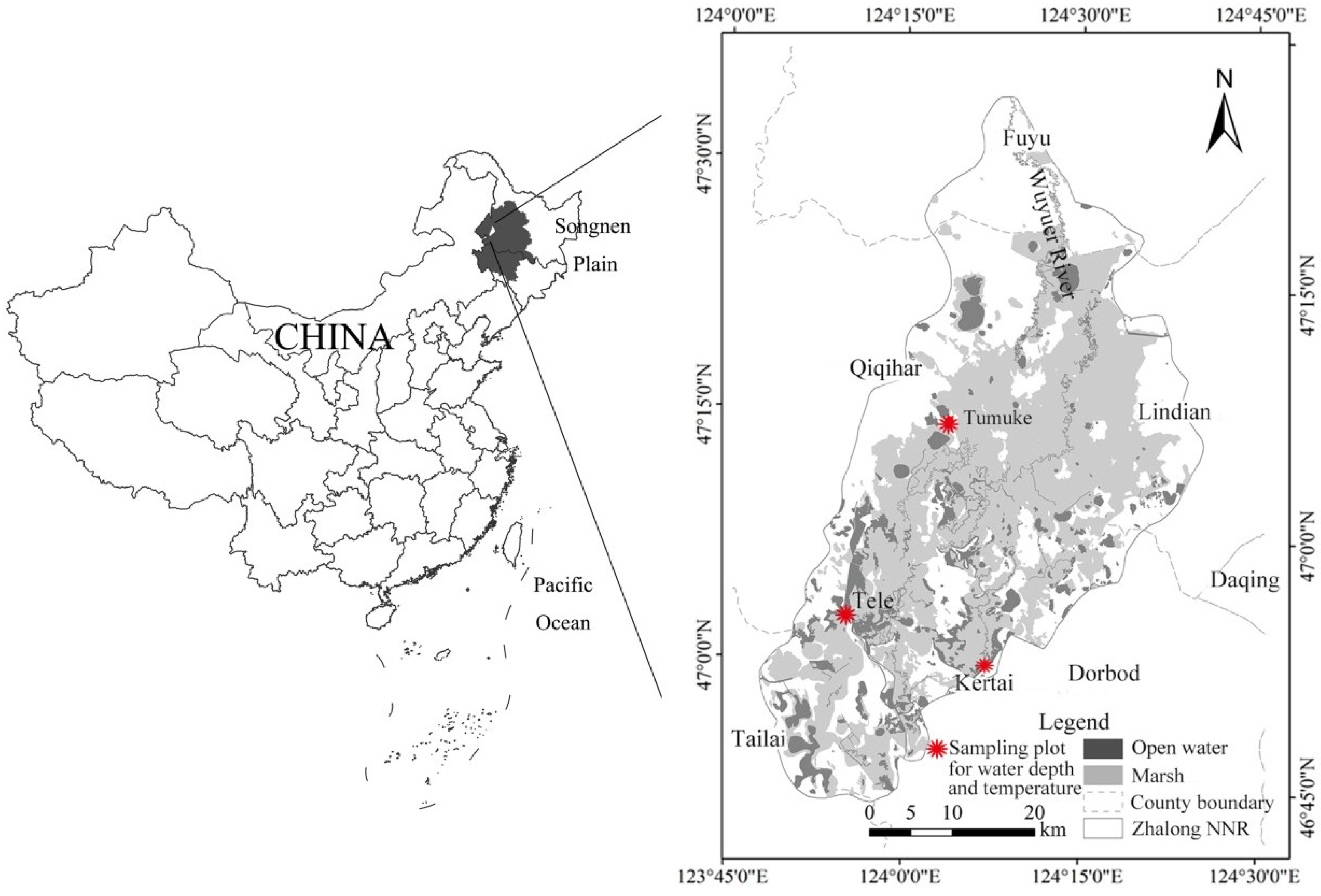
Figure 2.
Backscattering coefficients of Radarsat-2 HH and HV for different flooding situations (OW = open water, SAV = submerged aquatic vegetation, EAV = emerged aquatic vegetation, BS = bare soil) in 2015.
Figure 2.
Backscattering coefficients of Radarsat-2 HH and HV for different flooding situations (OW = open water, SAV = submerged aquatic vegetation, EAV = emerged aquatic vegetation, BS = bare soil) in 2015.
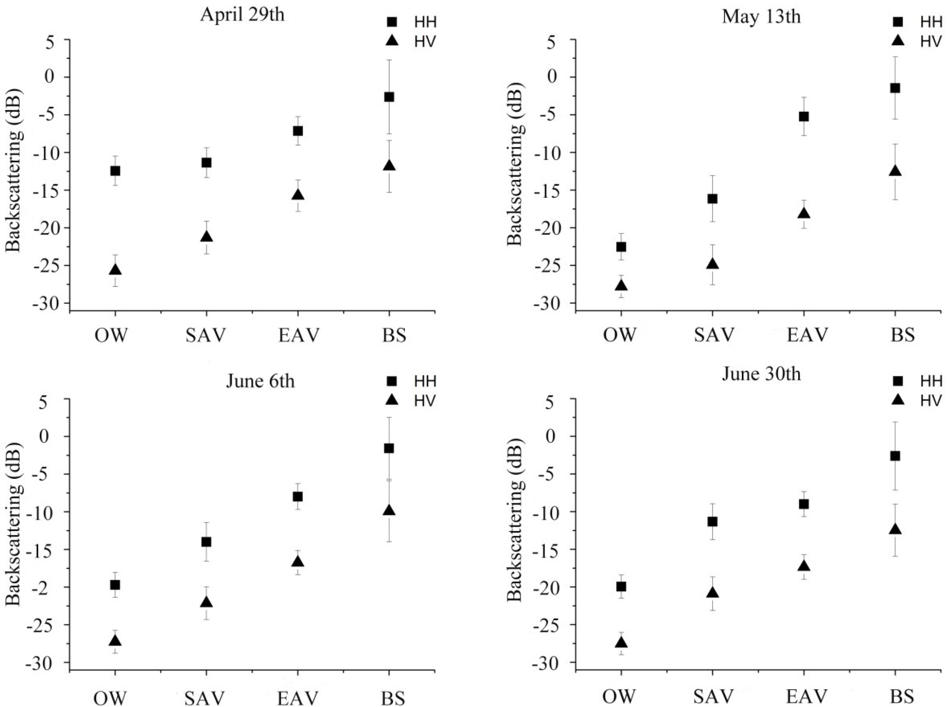
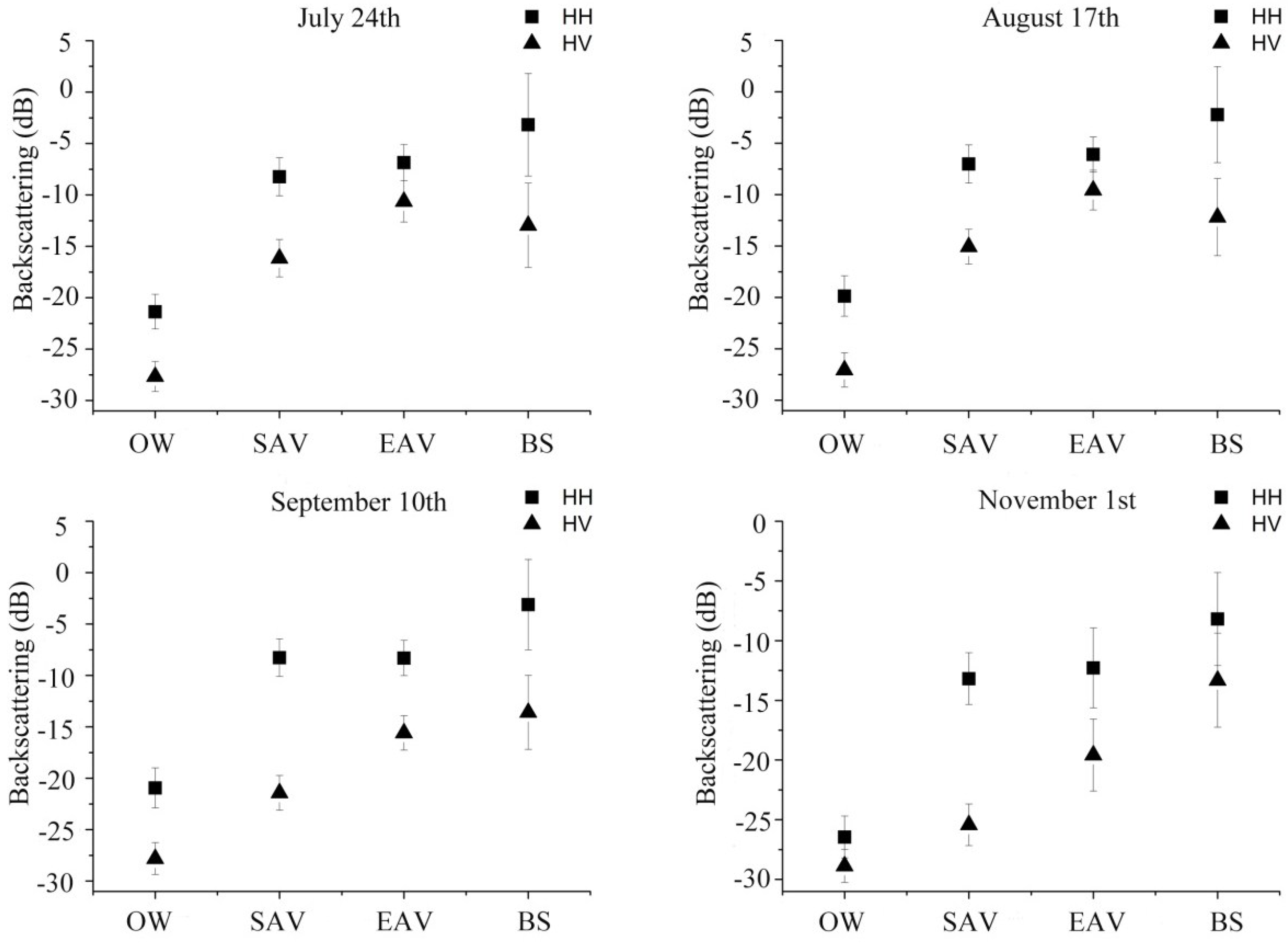
Figure 3.
Dynamics of the flood inundation extent in Zhalong wetlands over the 2015 hydrological year, blue color represents the inundation extent.
Figure 3.
Dynamics of the flood inundation extent in Zhalong wetlands over the 2015 hydrological year, blue color represents the inundation extent.
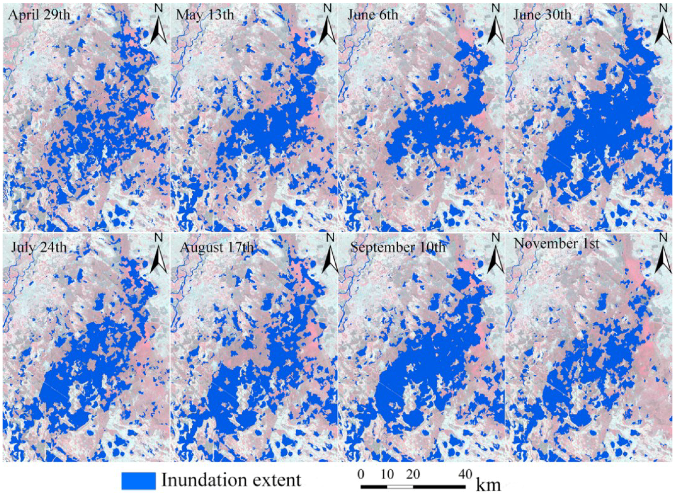
Figure 4.
Monthly dynamics of the flooding extent derived from multitemporal Radarsat synthetic aperture radar (SAR) images and water level derived from hydrological station in 2015.
Figure 4.
Monthly dynamics of the flooding extent derived from multitemporal Radarsat synthetic aperture radar (SAR) images and water level derived from hydrological station in 2015.
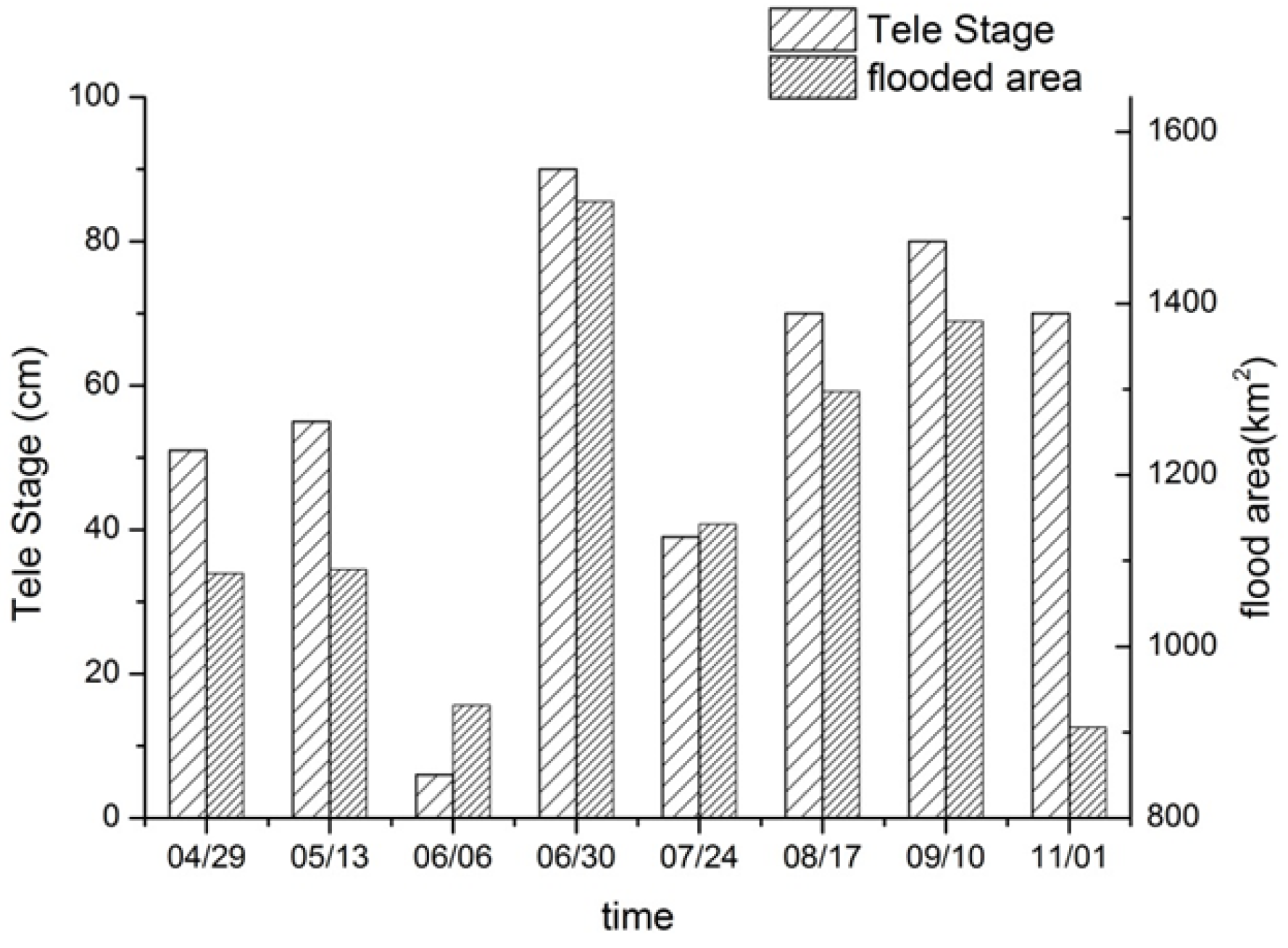
Figure 5.
(a) The flooding frequency map; and (b) the zoomed-in area of A; (c) an in situ snapshot of the area B and C in 15 May 2015.
Figure 5.
(a) The flooding frequency map; and (b) the zoomed-in area of A; (c) an in situ snapshot of the area B and C in 15 May 2015.

Figure 6.
The random forest (RF) classification results based on OLI (operational land imager) + SAR (synthetic aperture radar) + HRF (hydrological regimes features) model.
Figure 6.
The random forest (RF) classification results based on OLI (operational land imager) + SAR (synthetic aperture radar) + HRF (hydrological regimes features) model.

Figure 7.
Normalized variable importance scores for random forest classification based on OLI + SAR + HRF model.
Figure 7.
Normalized variable importance scores for random forest classification based on OLI + SAR + HRF model.


Table 1.
Accuracies of the single-temporal flood situation classification results (OW = open water, SAV = submerged aquatic vegetation, EAV = emerged aquatic vegetation, BS = bare soil).
Table 1.
Accuracies of the single-temporal flood situation classification results (OW = open water, SAV = submerged aquatic vegetation, EAV = emerged aquatic vegetation, BS = bare soil).
| Time | Accuracy | OW | SAV | EAV | BS | OA (%) | Kappa |
|---|---|---|---|---|---|---|---|
| 04/29 | UA (%) | 100 | 95.40 | 76.71 | 97.58 | 87.87 | 0.82 |
| PA (%) | 66.89 | 95.43 | 97.02 | 47.01 | |||
| 05/13 | UA (%) | 100 | 95.57 | 98.40 | 100 | 97.77 | 0.96 |
| PA (%) | 96.88 | 99.51 | 97.91 | 83.06 | |||
| 06/06 | UA (%) | 100 | 98.84 | 86.49 | 100 | 94.56 | 0.92 |
| PA (%) | 99.75 | 75.91 | 99.76 | 80.19 | |||
| 06/30 | UA (%) | 99.92 | 67.63 | 78.40 | 100 | 82.86 | 0.75 |
| PA (%) | 97.85 | 85.41 | 71.25 | 98.46 | |||
| 07/24 | UA (%) | 100 | 99.52 | 80.94 | 100 | 95.24 | 0.92 |
| PA (%) | 97.68 | 99.93 | 99.37 | 60.62 | |||
| 08/17 | UA (%) | 99.93 | 99.51 | 63.59 | 100 | 82.91 | 0.76 |
| PA (%) | 99.88 | 68.06 | 99.90 | 49.51 | |||
| 09/10 | UA (%) | 99.98 | 98.53 | 96.94 | 99.87 | 98.24 | 0.97 |
| PA (%) | 99.03 | 99.97 | 99.63 | 84.73 | |||
| 11/01 | UA (%) | 100 | 99.77 | 81.05 | 100 | 94.31 | 0.91 |
| PA (%) | 98.02 | 89.57 | 99.91 | 99.20 |
Table 2.
Error rates for classification accuracies of OLI + SAR + HRF model and OLI + SAR model.
| Omission Error (%) | Commission Error (%) | |||
|---|---|---|---|---|
| OLI + SAR + HRF | OLI + SAR | OLI + SAR + HRF | OLI + SAR | |
| Cultivated land | 14.01 | 13.22 | 0.71 | 6.39 |
| Meadow | 3.01 | 3.01 | 51.27 | 77.34 |
| Marsh | 2.88 | 52.14 | 1.88 | 3.28 |
| Water | 0.84 | 0.84 | 1.57 | 1.57 |
| Residential area | 5.82 | 5.48 | 0.65 | 0.41 |
| Saline and alkaline land | 4.44 | 4.44 | 52.31 | 48.30 |
| Overall accuracy (%) | 91.73 | 76.49 | ||
| Kappa | 0.88 | 0.67 | ||
© 2018 by the authors. Licensee MDPI, Basel, Switzerland. This article is an open access article distributed under the terms and conditions of the Creative Commons Attribution (CC BY) license (http://creativecommons.org/licenses/by/4.0/).
Share and Cite
MDPI and ACS Style
Na, X.; Zang, S.; Wu, C.; Tian, Y.; Li, W. Hydrological Regime Monitoring and Mapping of the Zhalong Wetland through Integrating Time Series Radarsat-2 and Landsat Imagery. Remote Sens. 2018, 10, 702. https://doi.org/10.3390/rs10050702
AMA Style
Na X, Zang S, Wu C, Tian Y, Li W. Hydrological Regime Monitoring and Mapping of the Zhalong Wetland through Integrating Time Series Radarsat-2 and Landsat Imagery. Remote Sensing. 2018; 10(5):702. https://doi.org/10.3390/rs10050702
Chicago/Turabian StyleNa, Xiaodong, Shuying Zang, Changshan Wu, Yang Tian, and Wenliang Li. 2018. "Hydrological Regime Monitoring and Mapping of the Zhalong Wetland through Integrating Time Series Radarsat-2 and Landsat Imagery" Remote Sensing 10, no. 5: 702. https://doi.org/10.3390/rs10050702
Note that from the first issue of 2016, this journal uses article numbers instead of page numbers. See further details here.