Studying Ionosphere Responses to a Geomagnetic Storm in June 2015 with Multi-Constellation Observations

1
School of Instrumentation Science and Opto-electronics Engineering, Beihang University, Beijing 100191, China
2
Abdus Salam International Centre for Theoretical Physics, Telecommunications/ICT for Development Laboratory, 34151 Trieste, Italy
3
School of Civil and Environmental Engineering, University of New South Wales, Sydney, NSW 2052, Australia
*
Author to whom correspondence should be addressed.
Remote Sens. 2018, 10(5), 666; https://doi.org/10.3390/rs10050666
Submission received: 1 February 2018
/
Revised: 15 April 2018
/
Accepted: 17 April 2018
/
Published: 25 April 2018
(This article belongs to the Special Issue Multi-Constellation Global Navigation Satellite Systems: Methods and Applications)
Abstract
:The Global Navigation Satellite System (GNSS) observations with global coverage and high temporal and spatial resolution, provide abundant and high-quality Earth-ionosphere observations. By calculating the total electron content (TEC), estimations from GNSS observables global and regional ionosphere TEC morphology can be further investigated. For the multiple constellation case, the numbers of ionosphere pierce points (IPP) has increased tremendously, and it is worth studying the features of the GNSS derived TEC under geomagnetic storms to show the benefits of multiple constellation measurements. With the Multi-GNSS Experiment (MGEX) observation data, ionosphere TEC responses to the geomagnetic storm on the 22 June 2015 were well studied. TEC perturbations were discovered, accompanied by ionosphere irregularities concentrating in high and middle latitudes. Through analysis of multi-GNSS observations, the Rate of TEC Index (ROTI) perturbations were proved to be generated by the geomagnetic storm, with simultaneous behaviors at different local times around the world, also indicating ionosphere scintillation. The ionosphere spatial gradient was also discussed with two short baseline MGEX sites; the maximum ionosphere gradient of 247.2 mm/km was found, due to ionosphere irregularity produced by the storm. This research has discussed ionosphere responses to geomagnetic storms with multi-GNSS data provided and has analyzed the availability of multi-GNSS observations to investigate ionosphere irregularity climatology. The proposed work is valuable for further investigation of GNSS performances under geomagnetic storms.
1. Introduction
The variation of the total electron content (TEC) of earth’s ionosphere can be mainly attributed to geomagnetic disturbances, during which magnetosphere electric fields penetrate into the ionosphere, changing the electron density and leading to ionosphere reactions. Linked with the interplanetary magnetic field, the dayside positive ionospheric responses are generated by the eastward prompt penetration electric field and the equator-ward neutral wind, while the negative ionosphere responses are generated by the more complex compositional effects of neutral winds. Moreover, with the energy injection by Joule heating at the polar region, the ionosphere responses for the geomagnetic disturbances usually initiate from the polar region and then propagate to the middle and low latitudes, accompanied with the modification of the local atmosphere conditions, causing ionosphere anomalies which are comprehensively observed and discussed.
Generally, ionosphere responses to geomagnetic storms can be concluded into three categories: (1) TEC variations and the expansion of the aurora oval due to particle precipitation. TEC and Rate of TEC Index (ROTI) behaviors in high latitudes under long-lasting particle precipitations have been analyzed, indicating enhancements of the ROTI accompanied with TEC variations [1]. Researchers have also gotten similar results by studying the Global Navigation Satellite System (GNSS) data collected in Canada during moderate storms in 2012 [2]. (2) The expansion of the equatorial ionization anomaly (EIA), further leading to hemisphere asymmetry in response to the storm. For the case of the 2015 St. Patrick’s Day storm, positive storm effects were found and considered to be related to different inputs of energy indicated by the AE magnetic index [3]. The negative storm effects were discovered mainly in the middle and high latitudes and were further verified with BDS observations [4]. For the 2013 October case, ROTI inhibition was discovered during the storm phase [5]. The research in Reference [6] indicated that the prompt penetration of the electric field (PPEF) played an important role at the beginning of the storm in the equatorial and low latitude regions. The vertical TEC (VTEC) behaviors during the storm were both influenced by PPEF and the disturbance dynamo electric field (DDEF). (3) The redistribution of particle densities above the ionosphere and the reshaping of ionosphere irregularities. According to Aarons’ criterion, the triggering of the ionosphere irregularities under geomagnetic storms closely depends on the geophysical location, the local time, and the geomagnetic intensity. This indicates that the effects of the geomagnetic storm on the ionosphere irregularities can be double-sided [7,8]. The positive effects trigger plasma bubble generation and severe ionosphere scintillations that are observed during geomagnetic storms. Middle-latitude ionosphere irregularities were investigated in association with the November 2004 storm [9]. A supper bubble was discovered from the June 2015 storm, with evidences of ion density decreasing and ROTI enhancements [10]; the negative effects for the evolutions of the plasma bubble were also discovered during the St. Patrick’s Day storm, stating that the force of the storm even blew away existing irregularities [11]. Another study was also conducted on the formation of the equatorial spread F, where irregularities and bubbles usually existed under intensive geomagnetic storms [12].
Based on the above responses, the change of ionosphere due to geomagnetic storms can further generate spatial and temporal ionosphere gradients, presented by the temporal discontinuity and spatial decorrelation of the ionosphere delay. Those consequences have influences on trans-ionosphere satellite ranging and positioning signals, causing ranging errors for ground-based argumentation systems (GBAS) [13,14,15]. The ionosphere gradients under the storm case can exceed 400 mm/km, measured from a 5 km distance limited baseline, as previous research revealed [16]. Recently, a method was explored to measure a very short baseline ionosphere gradient and a gradient of 518 mm/km was discovered, caused by an ionosphere plasma bubble [17]. However, the details of the bubble structure were not well studied, based on the given satellite measurements. Moreover, since the plasma bubbles or the irregularities can easily generate ionosphere scintillation, cautions should be taken for the ionosphere gradient calculation, which has been omitted in previous literature.
The global coverage and the high temporal and spatial resolution GNSS ionosphere measurements provide abundant and high-quality Earth-ionosphere observables. By calculating the GNSS TEC estimation from GNSS observables, the global and regional ionosphere TEC morphology can be further investigated [18]. With the study of statistics of TEC enhancement and depletion, the ROTI was defined and used to describe the intensity of the ionosphere irregularities [19]. The resolution of the TEC estimation, to portray regional ionosphere variation, relies greatly on the spatial distribution of IPP. For the multiple constellation case, the amounts of ionosphere pierce points (IPP) have increased tremendously [20,21]. It is worth studying the features of the TEC derived from GNSS observables under geomagnetic storms, to show the benefits of the multiple constellation measurements. The geometry of the GNSS constellation also contributes to a better coverage of IPPs, with the mixed orbits of the BeiDou Navigation Satellite System (BDS), to the TEC derived from the BDS enriched spatial diversity of IPP observations, and to set new opportunities to comprehensively discover the variations of the ionosphere under geomagnetic storms. The Multi-GNSS Experiment (MGEX) set-up by the International GNSS Service (IGS) [22] aims to track, collate, and analyze all available GNSS measurements, including BDS, Galileo, as well as any space-based augmentation system (SBAS) of interest [23,24]. The MGEX provides a data source for pioneering studies on the assessments of multi-GNSS performance as well as related applications.
The geomagnetic storm caused by coronal mass ejection (CME) on 22 June 2015 is a typical case for this work. The geomagnetic storm has a minimum of −204 nT Dst index at sudden storm commencement, mainly lasting for two days [25,26]. It happened at the summer solstice, when the occurrence of the ionosphere irregularities is considered quite low at the middle and low latitudes, thus, setting a good background for the investigations of any unusual phenomena.
In this work, the ionosphere responses on 22 June 2015 geomagnetic storm are analyzed using multi-constellation GNSS observations from the MGEX data. The ionosphere irregularities morphology during the event is further investigated with abundant observations from GPS, GLONASS, and BDS measurements. The temporal and geophysical behaviors of TEC from 22 June to 23 June 2015 are analyzed. Section 2 describes the data representation and the proposed methodology. Section 3 presents the experiments conducted to verify the responses with aspects of ionosphere TEC variation and irregular ROTI behaviors. The results are discussed in Section 4, which is followed by Section 5 with concluding remarks.
2. Data Presentation
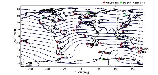
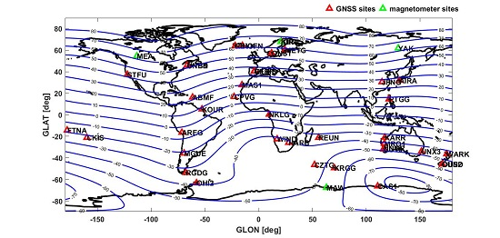
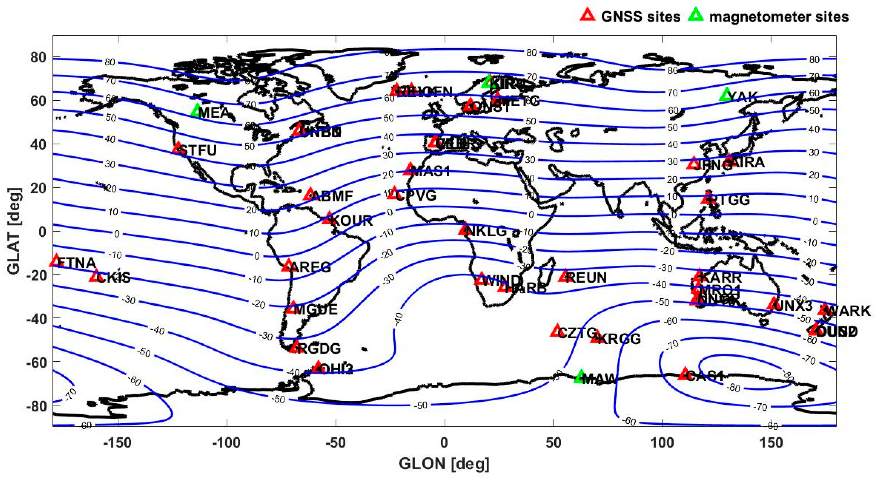
The ionosphere responses to the geomagnetic storm were mainly analyzed by multi-GNSS data from MGEX [27] (ftp://cddis.gsfc.nasa.gov/pub/gps/data/campaign/mgex/daily/), spanning from 22 June to 23 June at 2015. In comparison, the geomagnetic quiet days in June 2015 were also selected as a benchmark. The other supplementary data were divided by those subclasses: (1) data describing solar activities; mainly the solar wind speed measured by the Advanced Composition Explorer (ACE) in situ satellite; the interplanetary magnetic field (IMF) southward value, Bz, collected from an OMNI data website (https://omniweb.gsfc.nasa.gov/). (2) Data describing the geomagnetic index. Kp, Dst, AE, AU, and AL were collected from the International Service of Geomagnetic Indices (ISGI: http://isgi.unistra.fr/). Kp indicates the global daily geomagnetic perturbation; Dst indicates the intensity of the global geomagnetic disturbance; AE, as the initial of the auroral electrojet index, is used to measure the auroral zone magnetic activities produced by enhanced ionosphere currents though the auroral oval [28]; the AU and AL indexes serve as the upper/lower envelop of the H component disturbances observed in the auroral region; and AE represents the substitution between AU and AL (AE = AU − AL), demonstrating the eastward and westward electro-jets in the aurora region. (3) The ground geomagnetic data to measure the local geomagnetic field, provided by the geomagnetic world data center (http://www.wdc.bgs.ac.uk/catalog/master.html). (4) The Global Ionosphere Maps (GIMs) as an IGS product (ftp://gssc.esa.int/gnss/products/ionex/), to produce the global features of TEC and TEC variations. The observatories selected are demonstrated in Figure 1, where the captions GLON and GLAT indicate the geophysical longitude and geophysical latitude, the blue isoclines indicate the isoclines of geomagnetic latitudes.
2.1. Calculation of the TEC and ROTI
The ground GNSS observations are used to derive the TEC in the path between the GNSS satellite and a given receiver, and each satellite has slant TEC (STEC) according to its motion and coordinate related to the receiver. The ionosphere is considered a thin shell with a fixed height, where the TEC is concentrated and the absolute slant TEC can be produced to measure the status of the ionosphere at a given IPP. The proposed TEC calculation method is referred to as Ciraolo et al. (2007)’s arc-offset method [29] and realized by the software by the T/ICTD Lab of International Centre for Theoretical Physics. The detailed method is implemented as follows.
For a given satellite and epoch, there are phases (L1, L2) and the pseudo-ranges (P1, P2) at the two dual carriers. Then, the following observation equations can be formed:
where denotes the slant TEC to be estimated; and denote the satellite and receiver code-delay inter-frequency biases (IFBs), with no ambiguity term; is the effect of noise and the multi-path for code-delay observations; is the effect of noise and the multi-path for carrier-phase observations ; and are the satellite and receiver IFBs for carrier-phase observations; and represents the bias produced by the carrier-phase ambiguities in the ionospheric observable.
Assuming a constant IBF, taking the average of the subtraction between Equations (1) and (2), we get Equation (3)
Note that Equation (3) neglects the noise and the multi-path on the carrier-phase observations .
By subtracting Equation (3) from Equation (2), the ambiguity term is removed from the carrier-phase ionospheric observable
Neglecting the noise term , Equation (4) is further written by
This formula describes the slant TEC affected by the bias terms; i = 1, 2, …, 32+ denotes available GNSS satellites; j = 1, …, denotes available receivers; t is all the available observation epochs (in one day or fraction, or many days). Arc is common to all continuous observations performed by receiver j on satellite i at times contiguous to t; is disregarded in the traditional approach but is basic for the alternative “arc-offset” solution. In Ciraolo’s method, the calibration is performed considering as functions of a set of unknown parameters |X|, forming the residuals
with the least-squares estimation method, the parameters |X| and unknown biases bi,p, bj,p, can be estimated together.
The overall procedures can be summarized as follows:
- Extraction of the un-calibrated slants from GNSS observations
- Quality control of the GNSS observations, elevation mask, arcs discontinuities, recovery of cycle slips, and so forth.
- Solve Equation (7) with the least-squares solution indicated by summation of Equation (6)
- Calculating the residuals of the solution
According to Reference [29], the residuals can vary from 1TECU to ~8TECU, depending on the conditions.
Vertical TEC denotes the mapping at the zenith and is derived by
where represents the averaging radius of the earth; is the elevation angle in radians; denotes the average height of IPP and is considered as 450 km.
To further describe the disturbance of the ionosphere TEC, the rate of the slant TEC index has been proposed, which takes the average standard deviation of the slant TEC rate, and is widely used by the researchers. The rate of the slant TEC is given as
where and are the slant TEC at the and time epochs; is the time interval. Usually, the unit of ROT is TECU/min. The ROTI is defined in Reference [19]:
where denotes the averaging ROT during epochs. Experimentally, a threshold of 0.2 TECU/min is set to determine whether an irregularity exists [19]. The relationship between the ROTI and the scintillation indices has already been well studied to verify the belief of the ROTI as a reliable indicator of ionosphere irregularity [30,31,32].
The disturbance of TEC is characterized by the percentage of TEC variation over the average TEC under the geomagnetic quiet condition (five geomagnetic quiet days in the same month were chosen according to the ISGI quiet days data, in this work, the days of year 156, 155, 153, 154 and 171, 2015. The order of these days are according to the geomagnetic quiet levels revealed by the ISGI quiet days data, by selecting the first five quiet days), expressed as
2.2. Calculation of Geomagnetic Perturbations
The geomagnetic perturbation is closely related to the horizon value variation of the local magnetic field and this can be further calculated by
where denotes the solar daily variation of the earth’s magnetic field related to the regular ionospheric dynamo. denotes the magnetic dip angle of the given location, represents the magnetic disturbance due to the disturbed ionosphere electric currents, represents SYM-H, the contributions of the electric currents in the magnetosphere (refer to Reference [1]).
2.3. Calculation of the Ionosphere Gradient
The ionosphere gradient is defined as the ionosphere delay between two adjacent points per kilometer and is usually analyzed for ionosphere influence on GBAS performance [33]. The two adjacent points are close enough to share the same visible satellites. During geomagnetic storms, the ionosphere can be significantly disturbed and a large spatial gradient can be generated. A gradient as much as 400 mm/km is considered a threat to GBAS, as previous work revealed [34]. Reference [35] found gradients as large as 413 mm/km that can be modeled as a plain semi-infinite wavefront. In South America, a large number of gradients exceeding ICAO’s threat model was reported, with a maximum value of 800 mm/km, referred to in Reference [36]. The causes of the ionosphere gradient can be multiple, such as traveling ionosphere disturbance and ionosphere irregularities. In Thailand, the ionospheric delay gradient can vary from about 28 to 178 mm/km, while 20 to 100 mm/km is frequently observed during the plasma bubble occurrences, according to Reference [37]. Therefore, the analysis of the ionospheric gradients can be a good criterion to characterize the ionospheric TEC spatial variations, detecting the inhomogeneity of the ion density and further indicating the ionosphere irregularity. The ionosphere gradient value is greatly influenced by elevation, thus, for physical modeling, the elevation angle should be selected above 30 degrees. In this work, the ionosphere gradient is calculated by Equation (13), where and are TEC estimations by Section 2.1, measured from two adjacent points (sites) in meters. is the distance between the two points. denotes the L1 band frequency of GNSS, typically 1575.42 MHz.
The overall procedure of the ionosphere gradient calculation is concluded as follows:
- The TEC calculation using raw GNSS carrier phase measurements, as Section 2.1 described.
- The TEC slips detection method of Astfayeva is implemented [38]; TEC slips are calculated by the difference of two adjacent epochs of calibrated slant TEC values; epochs with intervals of 30 s.
- Removing the TEC slips larger than the threshold for ionosphere gradient calculation; the threshold is set to be 2 TECU in the middle latitudes, 3TECU in the low latitudes and equatorials (refer to Reference [38]).
- Calculating the ionosphere gradient with Equation (13).
- The post-processing check for large gradient values, to exclude the gradients strongly influenced by cycle slips.
3. Results
3.1. Global Morphology of Geomagnetic Storms
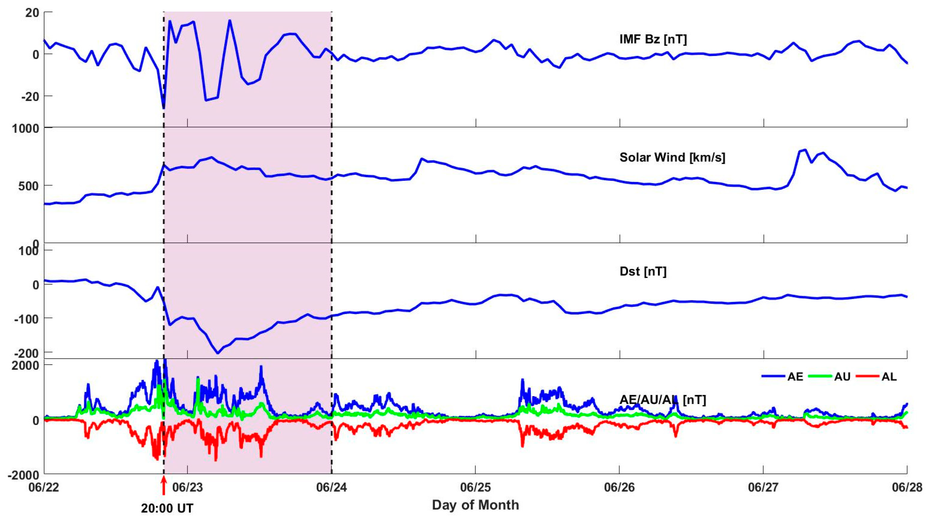
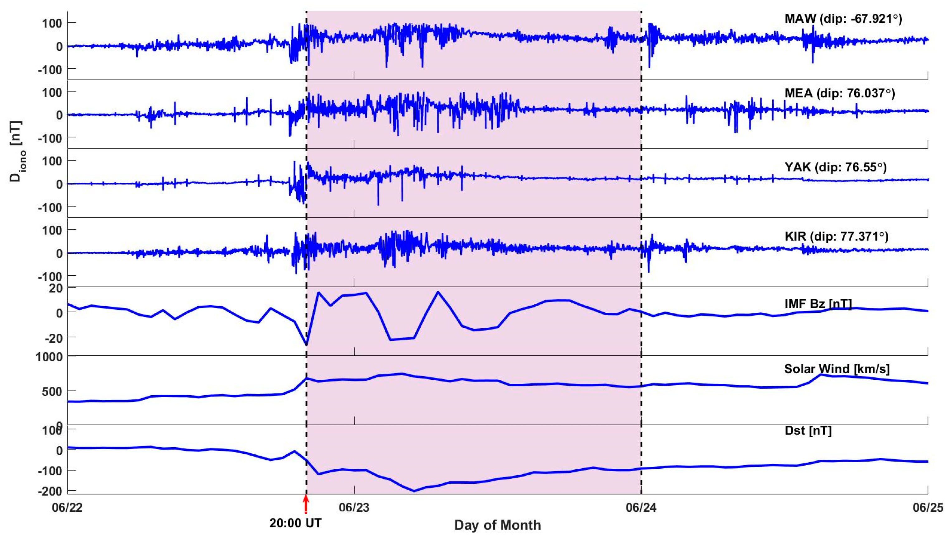
The global morphology of this geomagnetic storm was demonstrated in Figure 2. The solar wind component started increasing drastically at 20:00 UT 22 June 2015 and reached its maximum value of 742 m/s, 8 h later. The solar wind speed remained at a high level until 27 June 2015 and had another peak at 07:00 UT on 27 June. It then decreased gradually to be less than 400 km/s. The IMF Bz turned southward just a few minutes after the burst of solar wind and reached a minimum value of −26.3 nT at 20:00 UT. The IMF Bz oscillated with variations from the 22 to 23 June due to the rapid Alfven fluctuations. The minimum AL value was −1535 nT on the 23rd at 04:39 UT and the maximum AU value was 1503 nT on the 23rd at 01:46 UT. The Dst value dropped down to −204 nT during the second sub-phase of the storm on the 23rd at 05:00 UT. The perturbation of AE/AU/AL had several sub-patterns during the storm. The first perturbation sub-pattern started at 05:00 UT and lasted for 6 h, the AE peak value got to 1262 at 07:20 UT, and the minimum AL value dropped to −676. The second perturbation sub-pattern occurred at the commencement of the storm, the maximum AE reached 2083 nT around 20:20 UT, with the AL falling to −1058 nT. The AU demonstrated strong variations during this sub-pattern. The third perturbation sub-pattern was related to the second sub-phase of the storm, starting at midnight on the 23rd and lasting over 7.5 h. The AU reached a peak value of 1469 nT after 02:00 UT.
Several magnetic observatories (MAW, Mawson (67.604° S, 62.879° E); MEA, Meanook (54.616° N, 113.347° W); YAK, Yakutsk (61.96° N, 129.66° E); KIR, Kiruna (67.8428° N, 20.4201° E)) as shown in Figure 1 were selected at high latitudes, as the variation of shown in Figure 3. It showed that the geomagnetic fields at high latitudes oscillated drastically during the storm due to the influence of high-speed solar winds. This is in good consistency with previous discoveries of magnetic responses to high-speed solar winds at high latitudes regions [1,39], leading to ionosphere TEC variations. The asymmetry feature was also found between the northern hemisphere and southern hemisphere. In the southern hemisphere, only the MAW observatory had strong magnetic perturbations. The rest of the responses of the southern hemisphere were comparatively light. It is also demonstrated that the main phase of the geomagnetic perturbation was from 20:00 UT on 22nd to 15:00 UT on 23rd, similar to the behavior of AE/AU/AL in Figure 2, due to the ionosphere dynamo in the storm.
3.2. Global TEC Responses
With the IGS Ionosphere Map Exchange Format (IONEX) data, combined with the IGS Ionosphere Combination Center from JPL IONEX products [40,41], the global TEC responses were further analyzed. Figure 4a showed the global TEC variation for the American sector (longitude: 70° W), the European–African sector (longitude: 20° E), and the Asia–Australian sector (longitude: 130° E), respectively. It turns out that the European–African sector suffered from the event the most, keeping long TEC enhancements in EIA [42], which is consistent with previous results [43]. The increase of the TEC around the EIA regions in the European sector lasted for three days. The distortion of the equatorial crest was observed on the main phase of the storm and its recovery phase, however, the clear equatorial crest appeared again after 25 June. Similar characteristics were observed in Figure 4b, demonstrating the variation of TEC differences. Background TEC was calculated using the most geomagnetic quiet days’ value in the same month. The TEC enhancement in the Asian–Australian sector was dominant on 23 June, with an obvious southward expansion of the EIA region. The TEC decrease was found in the American high latitudes on 23 June, indicating the TEC inhibitions during the geomagnetic convection.
3.3. Local TEC Responses from MGEX Observations
The STEC was represented in Figure 5 to distinguish the impact of the geomagnetic storm. Tremendous TEC enhancements were observed at the low latitudes of the southern hemisphere, compared with the northern hemisphere, indicating the asymmetrical reaction of the ionosphere during this storm. CUT0, NNOR, MOR1, and KARR had great STEC enhancements before 10:00 UT on the 23rd at local day sides within the same time zone. NRMG and CKIS were located east in another time zone and the TEC enhancements were also dominant until local midnight. The STEC from the BDS measurements were at the same level of those from the GPS and GLONASS, and it sometimes became the most dominant.
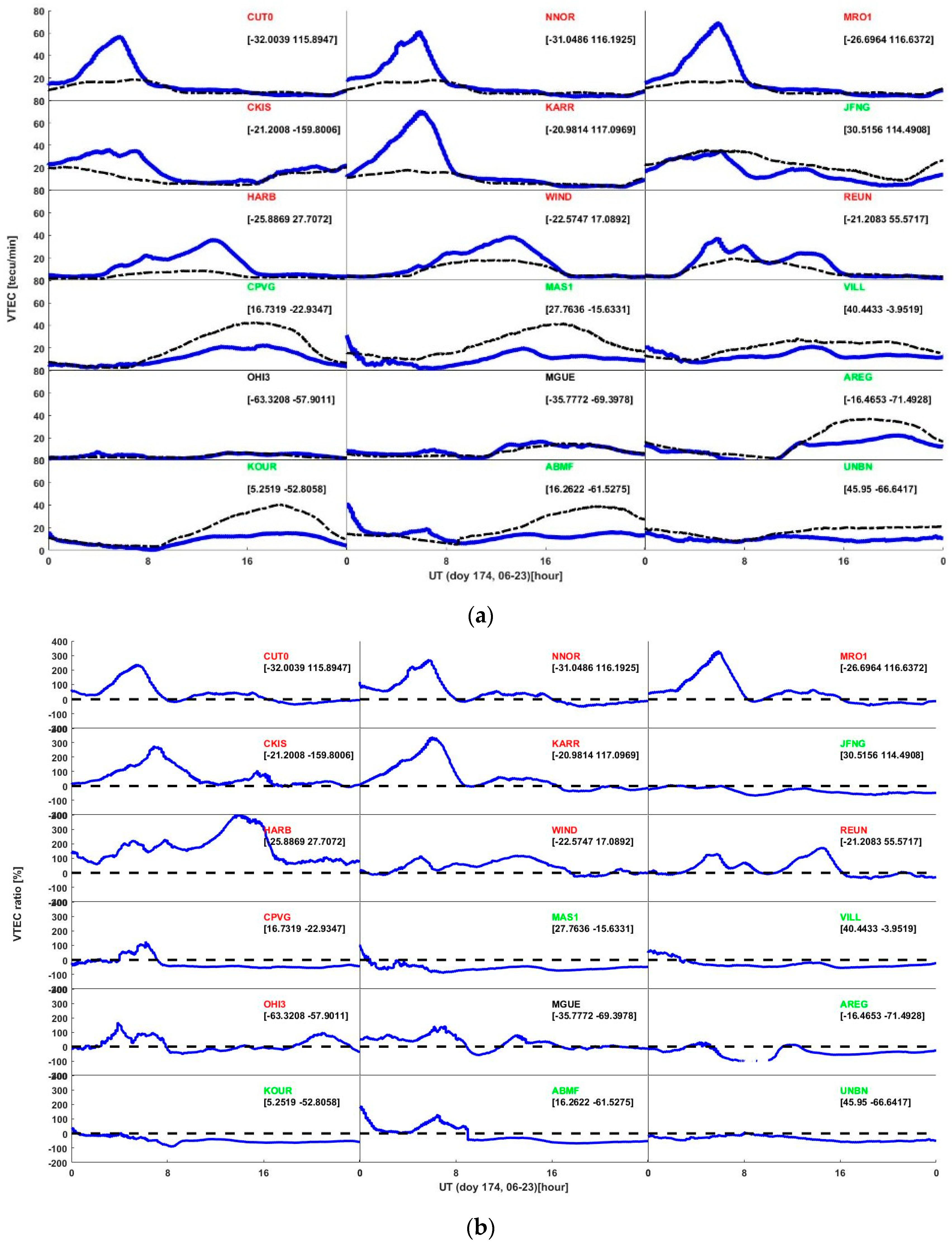
The calibrated VTEC was also considered. Figure 6 shows the VTEC enhancements at the Asian–Pacific, European–African, and American regions during the storm phase. In Figure 6a, the peak value occurred at ~05:20 UT in CUT0 and NNOR, at ~05:50 UT in MRO1 and KARR, and at ~06:50 UT in CKIS. For the European–African region, the TEC enhancements achieved a maximum value at ~13:20 UT in HARB and WIND and at 05:58 UT in REUN. However, the TEC depletions were also found in the northern hemisphere in Europe (CPVG and VILL), continuing for most of the day after the second sub-phase of the storm. Similar TEC depletions were also noticed at AREG, KOUR, and ABMF in the American region. The different times of the peak value in similar longitudes indicated the propagation of the TEC variations due to the storm. In Figure 6b, the maximum variation percentage reached up to 417% in the HARB station. The anomalies fit well with Figure 4b. It seems that the anomalies mainly occurred in the EIA regions, pushing EIA southward (Asian, Europe) or greatly inhibiting the EIA after the main phase of the storm (America). As consequences, the obvious positive storm effect was discovered in CUTO, NNOR, MRO1, and KARR in the Asian–Pacific region; the enhancements were also observed in HARB and WINDREUN in the southern hemisphere of the European–African region; depletions were found in CPVGand VILL in the northern hemisphere in the European–African region; and the inhibition effect was also observed in AREG, KOUR, and ABMF in the American region.
3.4. Local ROTI Variations
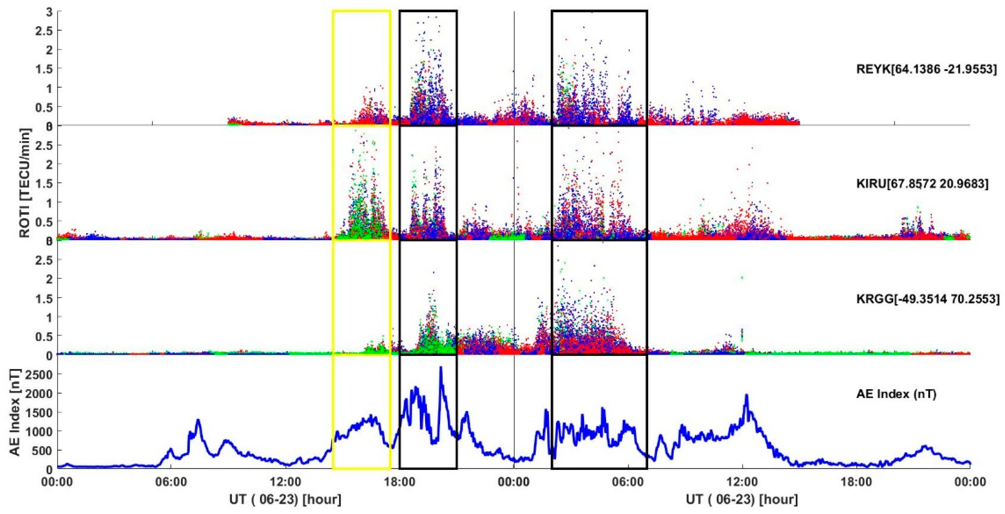
The TEC behavior observed from the MGEX observations indicates ionosphere scintillation. Thus, some ionosphere irregularities have been generated by this event. To further verify the characteristics of those irregularities, the following studies were focused on ROTI, calculated from the GPS, GLONASS, and BDS observations in the European sector. From 22 June, large ROTI values were observed in the European sector, which was in accordance with previous studies [17,44], concluding that a super plasma bubble was generated during the storm. With the benefits of the multi-GNSS observations, the phenomenon has been further verified. The enhancement of the ROTI during the storm can be contributed to two influential factors: (1) the aurora ovals expansion, with growth of particle precipitation, observed mainly at high latitudes, as Figure 7 demonstrated; (2) the prompt penetration of the electric field, observed mainly at the middle and low latitudes, and contributed largely to ionosphere irregularities at the middle latitudes.
In Figure 7, large ROTI values were observed simultaneously, with different time zones in 3 MGEX stations; this was one of the verifications that the storm-induced ionosphere irregularities. The ROTI variations took place mainly in two phases. The first phase started from 18:00 UT on the 22nd and lasted for around 3 h. The second phase started from 02:00 UT on the 23rd and gradually vanished after 06:00 UT. The ROTI values of different constellations shared similar temporal characteristics, further supporting the storm-induced ionosphere irregularities from another side. In REYK and KIRU, a pre-storm ROTI variation was observed from 15:00 UT to 17:00 UT, during the local sunset period.
The developing patterns of the ionosphere irregularities represented by the ROTI were shown in Figure 8. The red and pink rectangles indicated the location of large ionosphere irregularities, observed by the ROTI. Figure 8a demonstrates the ROTI enhancements in the first sub-phase of the storm and clear irregularity patterns were observed in 35° W–35° E, 55° N–72° N. The results were consistent with Figure 7. The intensity of the ionosphere irregularities increased in the second sub-phase of the storm, as Figure 8b shows. Another two irregularities appeared in the northern hemisphere, one in the eastern coast of USA and the other across Spain and northern Africa. The responses in the southern hemisphere were also positive. The irregularities were dominant in 90° W–130° W, 70° S–60° S, with almost a 40-degree longitudinal coverage. Another feature was highlighted in 45° E–77° E, 30° S–50° S, with increments of irregularities from the first sub-phase of the storm to the second sub-phase of the storm. Noticeable irregularities occurred in New Zealand, with a coverage of 160° E–180° E, 30° S–50° S. The ionosphere bubbles of this region were further investigated in Section 3.5.
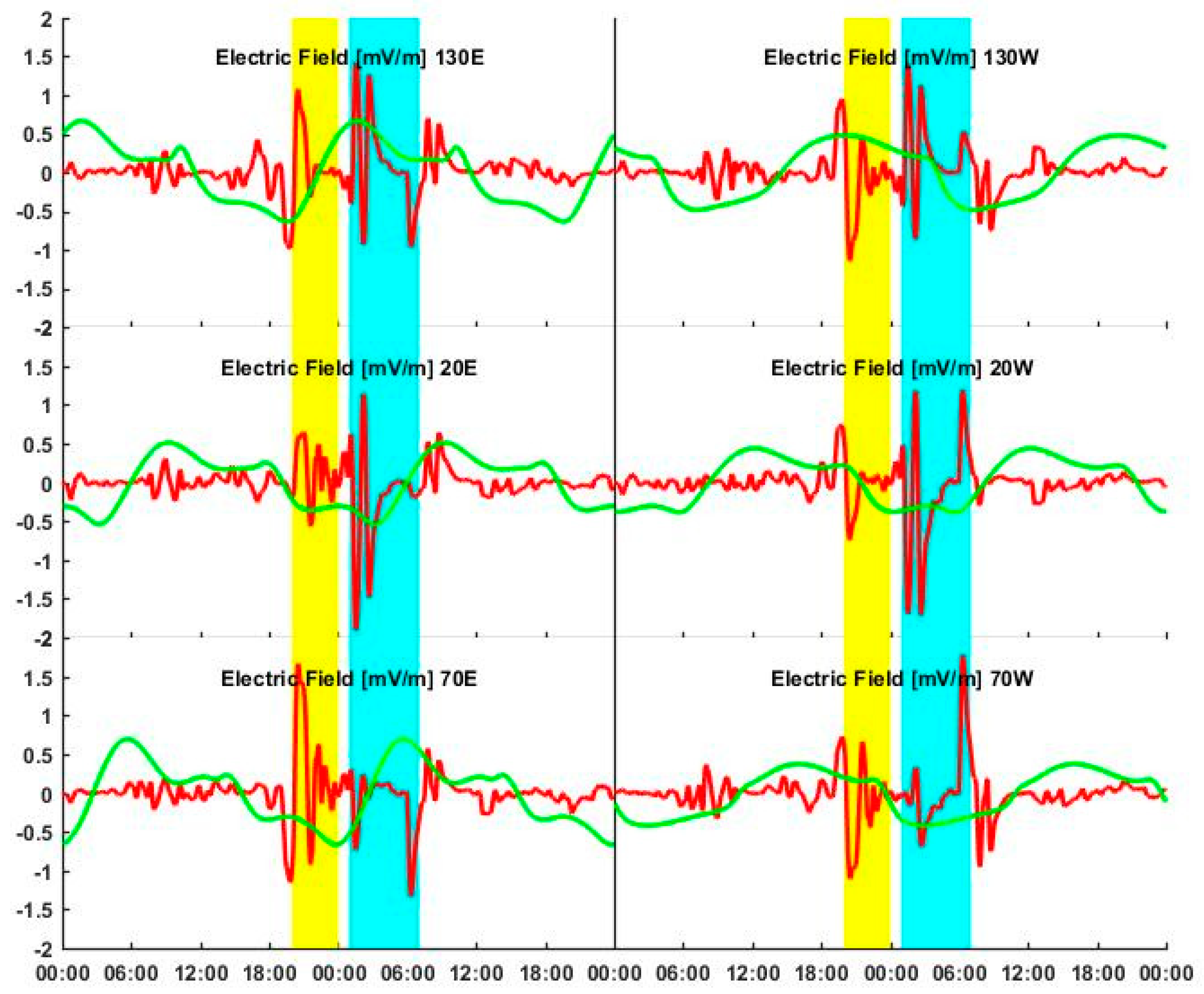
Those large-scale simultaneous triggers of the ionosphere irregularities in the middle latitudes, as Figure 8b demonstrates, were considered to be driven by the prompt penetration of electric field (PPEF, http://geomag.org/models/PPEFM/RealtimeEF.html) propagating through high latitudes to the middle and low latitudes. Figure 9 shows that the PPEF clearly had two dominant phases coordinated with the storm phases. The first sub-phase was at 20:00 UT on the 22nd to 00:00 UT on the 23rd, mainly affecting the eastern hemisphere. The PPEF varied greatly over the quiet electric field, in 20° E, 70° E, and 130° E, and then changed from westward to eastward in 20° W and 70° W, with less strength than those behaviors in the eastern conjugate points. The PPEF in 130° W was in a similar level as that in 130° E. The second sub-phase was from 02:00 UT to 06:00 UT on the 23rd, with stronger intensities of PPEF and leading to the second largest scale ROTI enhancements globally, in accordance with Figure 8b. The asymmetry features were noticed between the eastern hemisphere and the western hemisphere. The PPEF were considered the main cause of the EIA behavior shown in Figure 4 for the Asian–Australian sector, pushing the F layer ionosphere toward the higher latitudes of the southern hemisphere. The PPEF gradually decreased after 06:00 UT on the 23rd.
3.5. The Effect on the Ionosphere Spatial Gradient
Two MGEX sites, OUS2 and DUND, with a distance of 9.585 km, were selected to study the effect of this storm on the ionosphere spatial gradient. Figure 10 demonstrated the spatial gradient obtained from the GPS/GLONASS observations. The different colors denoted different satellites. All the ionosphere anomaly gradients discovered during the storm were collected and a total number of 59 satellites were considered. Figure 10a showed the ionosphere spatial gradient at one of the geomagnetic quiet days in the month (day of year (doy) 156), and the ionosphere spatial gradient was evenly distributed in accordance to the time (UT) and the maximum gradient below 15 mm/km, which is reasonable according to previous investigations [14,34]. Figure 10b shows the ionosphere spatial gradient during the main phase of the storm (doy 174), and the huge variation of the ionosphere spatial gradient was discovered from 02:00 UT to 07:30 UT, with the maximum value approaching 250 mm/km. The minus sign denotes a decrease. After 08:00 UT, the ionosphere spatial gradient gradually recovered to its normal status. The results fit well with the results discussed in Section 3.4.
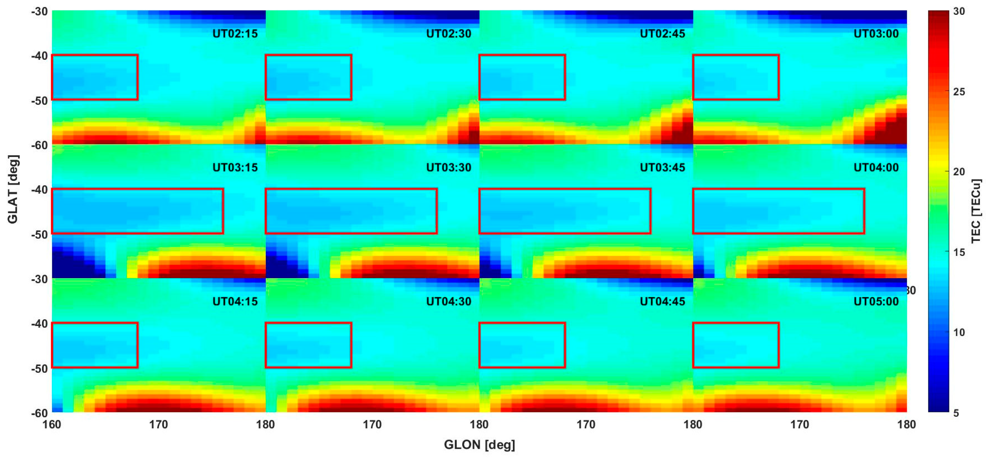
The maximum ionosphere spatial gradient was analyzed as Figure 11 shows; the maximum ionosphere spatial gradient occurred at GPS PRN 32 with a magnitude of 247.2 mm/km, around 04:00 UT, when the second sub-phase of the storm was dominant. The large ionosphere gradient was possibly related to the ionosphere irregularity during the second sub-phase of the storm, covering 160° E–170° E, 40° S–50° S, as demonstrated in Figure 8b. In Figure 12, the related IPP locations covered 164° E–168° E, 48° S–46° S. The dramatic variations of the ionosphere gradient shown in Figure 12 indicate the bubble effect on the trans-ionosphere GNSS signals, leading to the ROTI enhancement.
A regional TEC map was developed with ous2-dund observations, as Figure 12 demonstrated. A clear irregularity evolution was indicated from 02:15 UT to 05:00 UT, during the second sub-phase of the storm. The bubble reached its maximum size in the longitudinal direction at around 03:30 UT and gradually shrunk until 05:00 UT. The morphology was in accordance with Figure 8. This revealed that the intensity of the ionosphere gradient is also related to the longitudinal coverage of the irregularity. The maximum gradient presented by PRN32 was located in the wider part of the irregularity.
4. Discussion
4.1. TEC Responses to the Geomagnetic Storm
The TEC during the storm revealed noticeable enhancements. The features demonstrated in Figure 4 and Figure 6 contributed to both the latitudinal and longitudinal dependences. EIA was noticed toward the southern hemisphere in the Asian–Australian sector (130° E) at 07:15 UT on 23 June. This was mainly due to the sudden direction change of the prompt penetration electric fields at the moment and the eastward increasing electric field lifting ionosphere towards higher latitudes, which were quite unique compared to the previous geomagnetic storms [3,4,5,6]. While ~12.5 TECU depletion was discovered in the American sector (70° W) at 20:00 UT on 23rd; The TEC depletion in the Europe–Africa sector even reached the equatorial region when the SYM-H dropped to its minimum value of −201 nT at 04:00 UT, 10 h after the SSC. Both two hemispheres were greatly impacted by the rapid variation of IMF Bz, treated as strong disturbances [26]. The VTEC values from the multi-GNSS observations demonstrated differences of different observations in contributing to the VTEC calibration. Eighteen stations in three longitudinal sectors were analyzed by using MGEX observations; a ~200% increase of TEC was noticed in the southern hemisphere in the Asian and European–African sectors, while clear TEC depletions were noticed in AREG, KOUR, and ABMF in the American sector. Similar TEC variations using BDS observations were described by Reference [4], discovering both positive and negative responses in the St. Patrick’s Day Storm. In summary, during the main phase of this storm, the Asian and southern hemisphere of the European sectors demonstrated TEC enhancement and the American sectors represented TEC inhibition.
4.2. Irregularities Generated by the Geomagnetic Storm
A large scale of irregularities have been produced by the event at high and middle latitudes. The results in Figure 7 were in accordance with the observations reported by Reference [45], through the investigation of CHAIN (Canadian High Arctic Ionospheric Network) data. The characteristics of the irregularities generated this time were different from those described in the previous studies, which was dominant in the scales and occurred on the June solstice, the rarest period for large-scale plasma bubbles. The ionosphere irregularities were discovered mainly after the commencement of the storm, with two sub-phases, as Figure 8 showed. The simultaneous behaviors from different locations further verified the storm influences on the ionosphere irregularities generations, in addition to the general ionosphere irregularity morphology indicated by [7,8]. With spaceborne observations from SWARM satellites launched by ESA, Astafyeva demonstrated the changes of equatorial electrojet (EEJ) under the main phase of the storm [25]. With similar observations, Reference [10] proved that a super-bubble located between 30° N and 40° N in Europe was generated by the storm and severe ROTI enhancements were found from 23:00 UT on 22nd to 02:00 UT on 23rd. Moreover, through the investigation in Section 3.4, the multi-GNSS derived ROTI showed intensive appearances of large-scale irregularities, and other concentrating ROTI enhancements were discovered from 02:00 UT to 06:00 UT on the 23rd at REYK, HOFN, KIRU, and METG in the high latitudes of the northern hemisphere, and CZTG, KRGG, and DUND in the middle latitudes of the southern hemisphere (for the winter hemisphere, refer to Reference [25]). In the second sub-phase of the storm, both the north and south hemispheres suffered from ionosphere irregularities at high latitudes, demonstrated in Figure 8b. The large-scale ionosphere irregularities were considered to be generated by prompt penetration of the electric field during the storm [46]. As explained in previous studies, PPEFs affects the ionosphere by lifting the ionosphere up to a higher latitude, producing a decrease of the plasma density at the bottom-side of the ionosphere. From this work, the occurrence of large-scale ionosphere irregularities had mainly two influential factors: (1) the expansion of the oval at high latitudes, accompanied with particle precipitation, which can be verified by results in the REYK, HOFN, and KIRU stations, as well as the enhancements of AE during the storm; (2) PPEFs affects produced by the storm and propagating through low latitudes to middle latitudes, which can be seen from the results of the CZTG, KRGG, and DUND stations.
4.3. Benefits from Multi-GNSS Observations
Multi-GNSS observations help to increase the spatial observations of the ionosphere and to better understand the local morphology of the ionosphere variations. This was also supported by Reference [21]. Cherniak and Zakharenkova used ~5800 ground GPS/GLONASS observations to generate latitudinal ROTI maps during the storm phase. In this work, the regional ROTI perturbations were generated by GPS/GLONASS/BDS observations. The benefits of the BD GEO VTEC measurements were partially due to the geostationary orbit dynamics, indicated by Reference [4], to clearly represent both the positive and negative TEC responses in March 2015’s storm. In this work, the ROTI calculated from the Multi-GNSS observations provided abundant information of ionosphere irregularities under the geomagnetic storm, to help understand the patterns and changes in the ionosphere irregularities, as Figure 8 and Figure 12 show. One of the challenges for multi-GNSS observations is the computation efficiency, especially for some real-time applications. Geng et al. [47] has proposed a rapid solution for fixed ambiguity calculation with the help of ionosphere delay corrections. According to the algorithm in Reference [47], similarly, precision positioning for the Multi-GNSS case is expected in real-time operation by improving the computation efficiency of the current TEC calibration method. Another extension of the TEC method used in this work was to achieve a better TEC calibration with the help of Multi-GNSS measurements, as Geng and Bock [48] stated, according to the relative study of GLONASS. An improved TEC calibration based on Ciraolo’s method will consider more influential factors, such as the bias produced by inhomogeneous receivers, the bias among the satellite constellations, and even the multipath impacts on the low elevation satellites. A probable high resolution regional TEC map with less than 1TECU error is to be generated with the combination of improved TEC calibration based on Ciraolo’s methodology and study of Reference [48]. The promising investigations are useful for the fine precise positioning and related PPP-RTK (Precision Point Positioning-Real Time Kinematic).
4.4. Cause of Large Ionosphere Spatial Gradients
The multi-GNSS observations provide further opportunity to get the high resolution of the spatial ionosphere description within a small scale region [49]. The storm at 22–23 June 2015 is typical in this solar cycle, and a larger spatial gradient can be acquired by analysis of the observations from different constellations. Two major ionosphere anomalies were contributed to large ionosphere spatial gradients: (1) the TEC enhancements as studied by Reference [16] during the superstorm in 2003 and (2) the ionosphere irregularities, as revealed in Section 3.5. An ionosphere gradient of 518 mm/km was discovered, generated by a plasma bubble [17]. However, the features of large ionosphere spatial gradients caused by irregularities were more complicated. With a short appearance time, the gradient feature may vary a lot and be hard to be modeled. With multi-GNSS observations, a clear irregularity evolution pattern generated by the second sub-phase of the storm was shown in Figure 12. The PPEFs were considered to be the major cause for the irregularity formation. The comprehensive analysis in Figure 11 and Figure 12 also indicated that the ionosphere gradient represented by GNSS observations largely rely on the longitudinal coverage of the irregularity. Previous studies proved that the ionosphere gradient is influenced by the ‘width of gradient’; the conclusion is based on GPS observations. In this work, the multi-GNSS observations help to achieve more detailed results by considering the geometry of the GNSS satellites and the geophysical climatology of the ionosphere irregularity.
5. Conclusions
In this study, multi-GNSS observations from MGEX data were used to investigate ionosphere responses to the geomagnetic storm in June 2015. The results have revealed some features as follows:
(1) With multi-GNSS observations, the ionosphere TEC variations in this geomagnetic storm have been better investigated. The European sector has the most severe response; the southern hemisphere of the European sector showed dramatic TEC enhancements. Some MGEX sites that were analyzed showed over 300% of TEC enhancements during the second sub-phase of the storm. Other obvious TEC enhancements were discovered in the southern hemisphere of the Asian sector, with ~200% TEC increases observed. The TEC inhibitions were found near the equatorial region in the American sector, influenced by the storm forces.
(2) The geomagnetic storm brings strong ionosphere irregularities to both hemispheres. The irregularities were mainly concentrated in the high latitudes, as consequences of the particle precipitations. The concentrated features of the irregularities were analyzed by the behavior of ROTI from multi-GNSS observations. Several supper bubbles were produced, especially during the second sub-phase of the storm. The irregularities had longitudinal extension tendency, covering almost 10 degrees in the east–west directions. The intense appearances of the bubbles in the middle latitudes were related with the propagation of the prompt penetration electric field.
(3) Two nearby cites were selected to analyze the ionosphere spatial gradient. A maximum gradient of 247.2 mm/km was found by GPS/GLONASS observations during the second sub-phase of the storm. The possible cause for this spatial gradient was one of the bubbles located in 160° E–170° E, 40° S–50° S. The influence and statistical features of the ionosphere spatial gradient generated by the irregularities on the GNSS performances was worth further investigation.
Author Contributions
Yang Liu, Jinling Wang and Chunxi Zhang conceived the study idea and designed the experiments. Yang Liu and Lianjie Fu developed the simulation platform and performed the experiments. Yang Liu, Jinling Wang drafted the manuscript. All authors read and approved the manuscript.
Acknowledgments
This work was supported by the National Key Research and Development Plan by Ministry of Science and Technology 2016YFC1402502, the National Natural Science Foundation of China Innovation Group 61521091 and National Natural Science Foundation of China under Grant 61771030, 61301087. The contribution is also supported by 2011 Collaborative Innovation Center of Geospatial Technology. The authors would like to thank the reviewers for their detailed and insightful comments and constructive suggestions. Special thanks should be given to China Scholarship Council for the great supports of this research. Y.L gives special thanks to Abdus Salam International Centre for Theoretical Physics during her stay at the Telecommunications/ICT for Development Laboratory of the Centre. Special thanks to all providers of data used in this research.
Conflicts of Interest
The authors declare no conflict of interest.
References
- Zaourar, N.; Amory-Mazaudier, C.; Fleury, R. Hemispheric asymmetries in the ionosphere response observed during the high-speed solar wind streams of the 24–28 August 2010. Adv. Space Res. 2017, 59, 2229–2247. [Google Scholar] [CrossRef]
- Prikryl, P.; Ghoddousi-Fard, R.; Thomas, E.G.; Ruohoniemi, J.M.; Shepherd, S.G.; Jayachandran, P.T.; Danskin, D.W.; Spanswick, E.; Zhang, Y.; Jiao, Y.; et al. GPS phase scintillation at high latitudes during geomagnetic storms of 7–17 March 2012—Part 1: The North American sector. Ann. Geophys. 2015, 33, 637–656. [Google Scholar] [CrossRef]
- Nava, B.; Rodríguez-Zuluaga, J.; Alazo-Cuartas, K.; Kashcheyev, A.; Migoya-Orué, Y.; Radicella, S.M.; Amory-Mazaudier, C.; Fleury, R. Middle- and low-latitude ionosphere response to 2015 St. Patrick’s Day geomagnetic storm. J. Geophys. Res. Space Phys. 2016, 121, 3421–3438. [Google Scholar] [CrossRef]
- Jin, S.; Jin, R.; Kutoglu, H. Positive and negative ionospheric responses to the March 2015 geomagnetic storm from BDS observations. J. Geod. 2017, 91, 1–14. [Google Scholar] [CrossRef]
- Azzouzi, I.; Migoya-Orue, Y.; Mazaudier, C.A.; Fleury, R.; Radicella, S.M.; Touzani, A. Signatures of solar event at middle and low latitudes in the Europe-African sector, during geomagnetic storms, October 2013. Adv. Space Res. 2015, 56, 2040–2055. [Google Scholar] [CrossRef] [Green Version]
- Mao, T.; Sun, L.; Hu, L.; Wang, Y.; Wang, Z. A case study of ionospheric storm effects in the Chinese sector during the October 2013 geomagnetic storm. Adv. Space Res. 2015, 56, 2030–2039. [Google Scholar] [CrossRef]
- Aarons, J.; Whitney, H.E.; Allen, R.S. Global morphology of ionospheric scintillations. Proc. IEEE 1982, 59, 159–172. [Google Scholar] [CrossRef]
- Forte, B.; Radicella, S.M.; Ezquer, R.G. A different approach to the analysis of GPS scintillation data. Ann. Geophys. 2002, 45, 551–561. [Google Scholar]
- Li, G.; Ning, B.; Zhao, B.; Liu, L.; Wan, W.; Ding, F.; Xu, J.S.; Liu, J.Y.; Yumoto, K. characterizing the 10 November 2004 storm-time middle-latitude plasma bubble event in Southeast Asia using multi-instrument observations. J. Geophys. Res. Space Phys. 2009, 114, 1–16. [Google Scholar] [CrossRef]
- Cherniak, I.; Zakharenkova, I. First observations of super plasma bubbles in Europe. Geophys. Res. Lett. 2016, 43, 11137–11145. [Google Scholar] [CrossRef]
- Carter, B.A.; Yizengaw, E.; Pradipta, R.; Retterer, J.M.; Groves, K.; Valladares, C.; Caton, R.; Bridgwood, C.; Norman, R.; Zhang, K. Global equatorial plasma bubble occurrence during the 2015 St. Patrick’s Day storm. J. Geophys. Res. Space Phys. 2016, 121, 894–905. [Google Scholar] [CrossRef]
- Ray, S.; Roy, B.; Das, A. Occurrence of equatorial spread F during intense geomagnetic storms. Radio Sci. 2015, 50, 563–573. [Google Scholar] [CrossRef]
- Rovira-Garcia, A.; Juan, J.M.; Sanz, J.; González-Casado, G.; Ibáñez, D. Accuracy of ionospheric models used in GNSS and SBAS: Methodology and analysis. J. Geod. 2016, 90, 229–240. [Google Scholar] [CrossRef]
- Bang, E.; Lee, J. Methodology of automated ionosphere front velocity estimation for ground-based augmentation of GNSS. Radio Sci. 2013, 48, 659–670. [Google Scholar] [CrossRef]
- Zhao, L.; Yang, F.; Li, L.; Ding, J.; Zhao, Y. GBAS Ionospheric Anomaly Monitoring Based on a Two-Step Approach. Sensors 2016, 16, 763. [Google Scholar] [CrossRef] [PubMed]
- Park, Y.S.; Zhang, G.; Pullen, S.; Lee, J.; Enge, P. Data-replay analysis of LAAS safety during ionosphere storms. Proc. ION GNSS 2007, 2007, 25–28. [Google Scholar]
- Saito, S.; Yoshihara, T. Evaluation of extreme ionospheric Total Electron Content (TEC) gradient associated with plasma bubbles for GNSS Ground-based Augmentation System (GBAS). Radio Sci. 2017, 52, 951–962. [Google Scholar] [CrossRef]
- Nykiel, G.; Zanimonskiy, Y.M.; Yampolski, Y.M.; Figurski, M. Efficient Usage of Dense GNSS Networks in Central Europe for the Visualization and Investigation of Ionospheric TEC Variations. Sensors 2017, 17, 2298. [Google Scholar] [CrossRef] [PubMed]
- Pi, X.; Mannucci, A.J.; Lindqwister, U.J.; Ho, C.M. Monitoring of global ionospheric irregularities using the Worldwide GPS Network. Geophys. Res. Lett. 1997, 24, 2283–2286. [Google Scholar] [CrossRef]
- Gao, Z.; Shen, W.; Zhang, H.; Niu, X.; Ge, M. Real-time Kinematic Positioning of INS Tightly Aided Multi-GNSS Ionospheric Constrained PPP. Sci. Rep. 2016, 6, 30488. [Google Scholar] [CrossRef] [PubMed]
- Ren, X.; Zhang, X.; Xie, W.; Zhang, K.; Yuan, Y.; Li, X. Global Ionospheric Modelling using Multi-GNSS: BeiDou, Galileo, GLONASS and GPS. Sci. Rep. 2016, 6, 33499. [Google Scholar] [CrossRef] [PubMed]
- Dow, J.M.; Neilan, R.E.; Rizos, C. The International GNSS Service in a changing landscape of Global Navigation Satellite Systems. J. Geod. 2009, 83, 191–198. [Google Scholar] [CrossRef]
- Guo, F.; Li, X.; Zhang, X.; Wang, J. The contribution of Multi-GNSS Experiment (MGEX) to precise point positioning. Adv. Space Res. 2016, 59, 2714–2725. [Google Scholar] [CrossRef]
- Gao, W.; Gao, C.; Pan, S.; Meng, X.; Xia, Y. Inter-System Differencing between GPS and BDS for Medium-Baseline RTK Positioning. Remote Sens. 2017, 9, 948. [Google Scholar] [CrossRef]
- Astafyeva, E.; Zakharenkova, I.; Alken, P. Prompt penetration electric fields and the extreme topside ionospheric response to the June 22–23, 2015 geomagnetic storm as seen by the Swarm constellation. Earth Planets Space 2017, 68, 152. [Google Scholar] [CrossRef]
- Reiff, P.H.; Daou, A.G.; Sazykin, S.Y.; Nakamura, R.; Hairston, M.R.; Coffey, V.; Chandler, M.O.; Anderson, B.J.; Russell, C.T.; Welling, D.; et al. Multispacecraft Observations and Modeling of the June 22/23, 2015 Geomagnetic Storm. Geophys. Res. Lett. 2016, 43, 7311–7318. [Google Scholar] [CrossRef]
- Montenbruck, O.; Steigenberger, P.; Prange, L.; Deng, Z.; Zhao, Q.; Perosanz, F.; Romero, I.; Noll, C.; Stürze, A.; Weber, G.; Schmid, R. The Multi-GNSS Experiment (MGEX) of the International GNSS Service (IGS)—Achievements, prospects and challenges. Adv. Space Res. 2017, 59, 1671–1697. [Google Scholar] [CrossRef]
- Davis, T.N.; Sugiura, M. Auroral electrojet activity index AE, and its universal time variations. J. Geophys. Res. Space Phys. 1966, 71, 785–801. [Google Scholar] [CrossRef]
- Ciraolo, L.; Azpilicueta, F.; Brunini, C.; Meza, A.; Radicella, S.M. Calibration errors on experimental slant total electron content (TEC) determined with GPS. J. Geod. 2007, 81, 111–120. [Google Scholar] [CrossRef]
- Cherniak, I.; Zakharenkova, I.; Krankowski, A. Approaches for modeling ionosphere irregularities based on the TEC rate index. Earth Planets Space 2014, 66, 165. [Google Scholar] [CrossRef]
- Sieradzki, R.; Paziewski, J. Study on reliable GNSS positioning with intense TEC fluctuations at high latitudes. GPS Solut. 2016, 20, 553–563. [Google Scholar] [CrossRef]
- Liu, K.; Li, G.; Ning, B.; Hu, L.; Li, H. Statistical characteristics of low-latitude ionospheric scintillation over China. Adv. Space Res. 2015, 55, 1356–1365. [Google Scholar] [CrossRef]
- Akala, A.O.; Doherty, P.H.; Carrano, C.S.; Valladares, C.E.; Groves, K.M. Impacts of ionospheric scintillations on GPS receivers intended for equatorial aviation applications. Radio Sci. 2012, 47, 1–11. [Google Scholar] [CrossRef]
- Seo, J.; Lee, J.; Pullen, S.; Enge, P.; Close, S. Targeted Parameter Inflation within Ground-Based Augmentation Systems to Minimize Anomalous Ionospheric Impact. J. Aircr. 2015, 49, 587–599. [Google Scholar] [CrossRef]
- Datta-Barua, S.; Lee, J.; Pullen, S.; Luo, M.; Ene, A.; Qiu, D.; Zhang, G.; Enge, P. Ionospheric Threat Parameterization for Local Area Global-Positioning-System-Based Aircraft Landing Systems. J. Aircr. 2010, 47, 1141–1151. [Google Scholar] [CrossRef]
- Lee, J.; Moonseok, Y.; Pullen, S.; Gillespie, J.; Mathur, N.; Cole, R.; Rodriguez de Souza, J.; Doherty, P.; Pradipta, R. Preliminary results from ionospheric threat model development to support GBAS operations in the Brazilian region. In Proceedings of the 28th International Technical Meeting of the ION Satellite Division, ION GNSS+ 2015, Tampa, Florida, 14–18 September 2015; pp. 1500–1506. [Google Scholar]
- Rungraengwajiake, S.; Supnithi, P.; Saito, S.; Siansawasdi, N.; Saekow, A. Ionospheric delay gradient monitoring for GBAS by GPS stations near Suvarnabhumi airport, Thailand. Radio Sci. 2015, 50, 1076–1085. [Google Scholar] [CrossRef]
- Astafyeva, E.; Yasyukevich, Y.; Maksikov, A.; Zhivetiev, I. Geomagnetic storms, super-storms and their impacts on GPS-based navigation systems. Space Weather Int. J. Res. Appl. 2014, 12, 508–525. [Google Scholar] [CrossRef]
- Astafyeva, E.; Zakharenkova, I.; Förster, M. Ionospheric response to the 2015 St. Patrick’s Day storm: A global multi-instrumental overview. J. Geophys. Res. Space Phys. 2015, 120, 9023–9037. [Google Scholar] [CrossRef]
- Komjathy, A.; Sparks, L.; Wilson, B.D.; Mannucci, A.J. Automated daily processing of more than 1000 ground-based GPS receivers for studying intense ionospheric storms. Radio Sci. 2016, 40, 1–11. [Google Scholar] [CrossRef]
- Roma-Dollase, D.; Hernández-Pajares, M.; Krankowski, A.; Kotulak, K.; Ghoddousi-Fard, R.; Yuan, Y.; Li, Z.; Zhang, H.; Shi, C.; Wang, C.; et al. Consistency of seven different GNSS global ionospheric mapping techniques during one solar cycle. J. Geod. 2017. [Google Scholar] [CrossRef]
- Appleton, E.V. Two Anomalies in the Ionosphere. Nature 1946, 157, 691. [Google Scholar] [CrossRef]
- Cherniak, I.; Zakharenkova, I. New advantages of the combined GPS and GLONASS observations for high-latitude ionospheric irregularities monitoring: Case study of June 2015 geomagnetic storm. Earth Planets Space 2017, 69, 66. [Google Scholar] [CrossRef]
- Jiao, Y.; Morton, Y.T. Comparison of the effect of high-latitude and equatorial ionospheric scintillation on GPS signals during the maximum of solar cycle 24. Radio Sci. 2015, 50, 886–903. [Google Scholar] [CrossRef]
- Prikryl, P.; Ghoddousi-Fard, R.; Kunduri, B.S.; Thomas, E.G.; Coster, A.J.; Jayachandran, P.T.; Spanswick, E.; Danskin, D.W. GPS phase scintillation and proxy index at high latitudes during a moderate geomagnetic storm. Ann. Geophys. 2013, 31, 805–816. [Google Scholar] [CrossRef]
- Wei, Y.; Zhao, B.; Li, G.; Wan, W. Electric field penetration into Earth’s ionosphere: A brief review for 2000–2013. Sci. Bull. 2015, 60, 748–761. [Google Scholar] [CrossRef]
- Geng, J.; Meng, X.; Dodson, A.H.; Ge, M.; Teferle, F.N. Rapid re-convergences to ambiguity-fixed solutions in precise point positioning. J. Geod. 2010, 84, 705–714. [Google Scholar] [CrossRef]
- Geng, J.; Bock, Y. GLONASS fractional-cycle bias estimation across inhomogeneous receivers for PPP ambiguity resolution. J. Geod. 2016, 90, 379–396. [Google Scholar] [CrossRef]
- Wang, C.; Shi, C.; Zhang, H.; Fan, L. Improvement of global ionospheric VTEC maps using the IRI 2012 ionospheric empirical model. J. Atmos. Sol.-Terr. Phys. 2016, 146, 186–193. [Google Scholar] [CrossRef]
Figure 1.
The locations of the Global Navigation Satellite System (GNSS) Multi-GNSS Experiment (MGEX) and the magnetometer sites selected by this work.
Figure 1.
The locations of the Global Navigation Satellite System (GNSS) Multi-GNSS Experiment (MGEX) and the magnetometer sites selected by this work.

Figure 2.
The geomagnetic morphology of the storm (listing the interplanetary magnetic field (IMF) southward value (Bz), solar wind, Dst/AE/AU/AL indices).
Figure 2.
The geomagnetic morphology of the storm (listing the interplanetary magnetic field (IMF) southward value (Bz), solar wind, Dst/AE/AU/AL indices).

Figure 3.
The magnetic perturbations from the high latitude local observations.

Figure 4.
The global total electron content (TEC) responses to the HSS ((a) TEC responses; (b) TEC difference responses).
Figure 4.
The global total electron content (TEC) responses to the HSS ((a) TEC responses; (b) TEC difference responses).
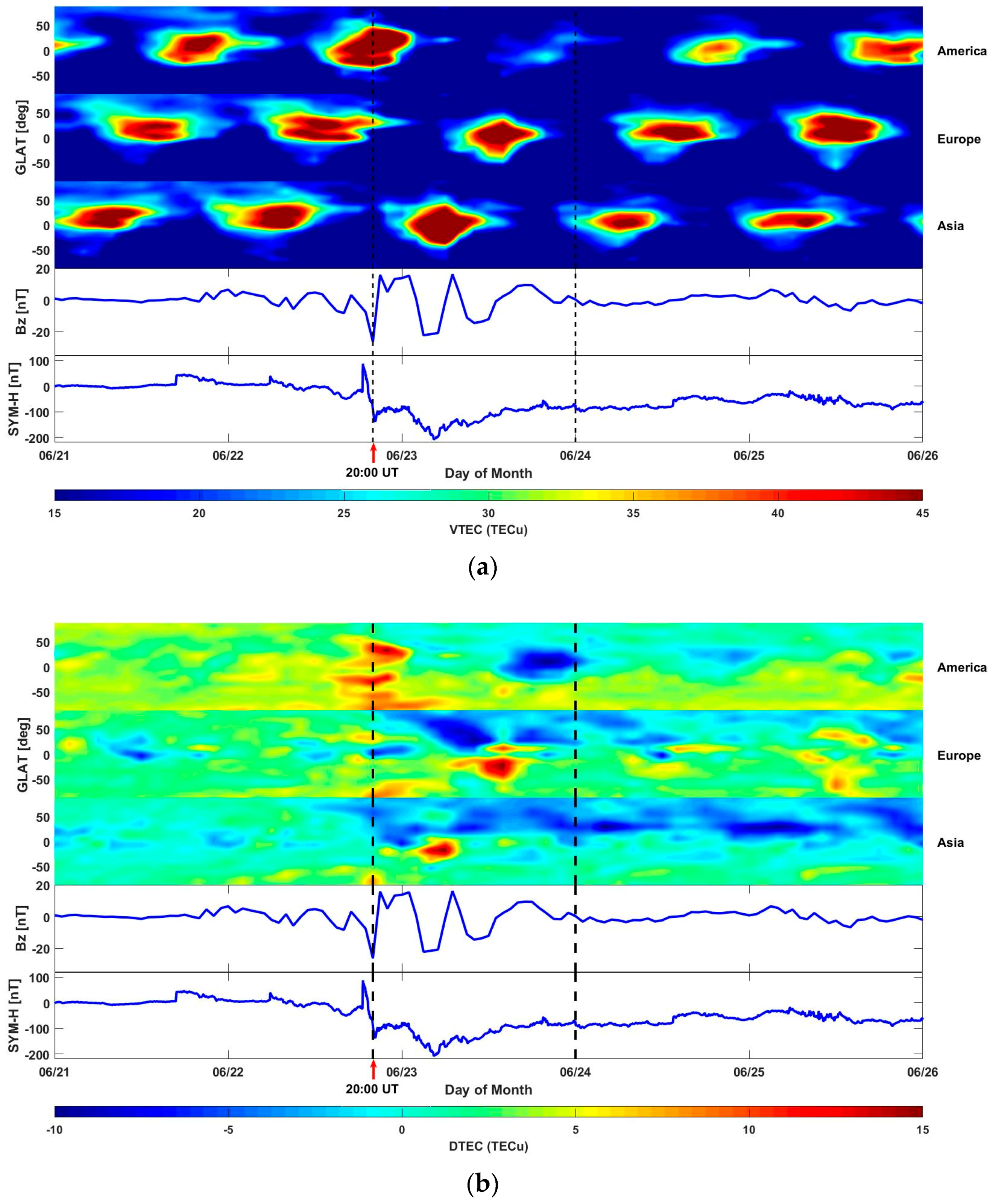
Figure 5.
The slant TEC (STEC) responses to the storm on 23 June (Multi-GNSS observations from MGEX data). (blue: GPS; red: GLONASS; green: BeiDou Navigation Satellite System (BDS); pink: GALILEO).
Figure 5.
The slant TEC (STEC) responses to the storm on 23 June (Multi-GNSS observations from MGEX data). (blue: GPS; red: GLONASS; green: BeiDou Navigation Satellite System (BDS); pink: GALILEO).
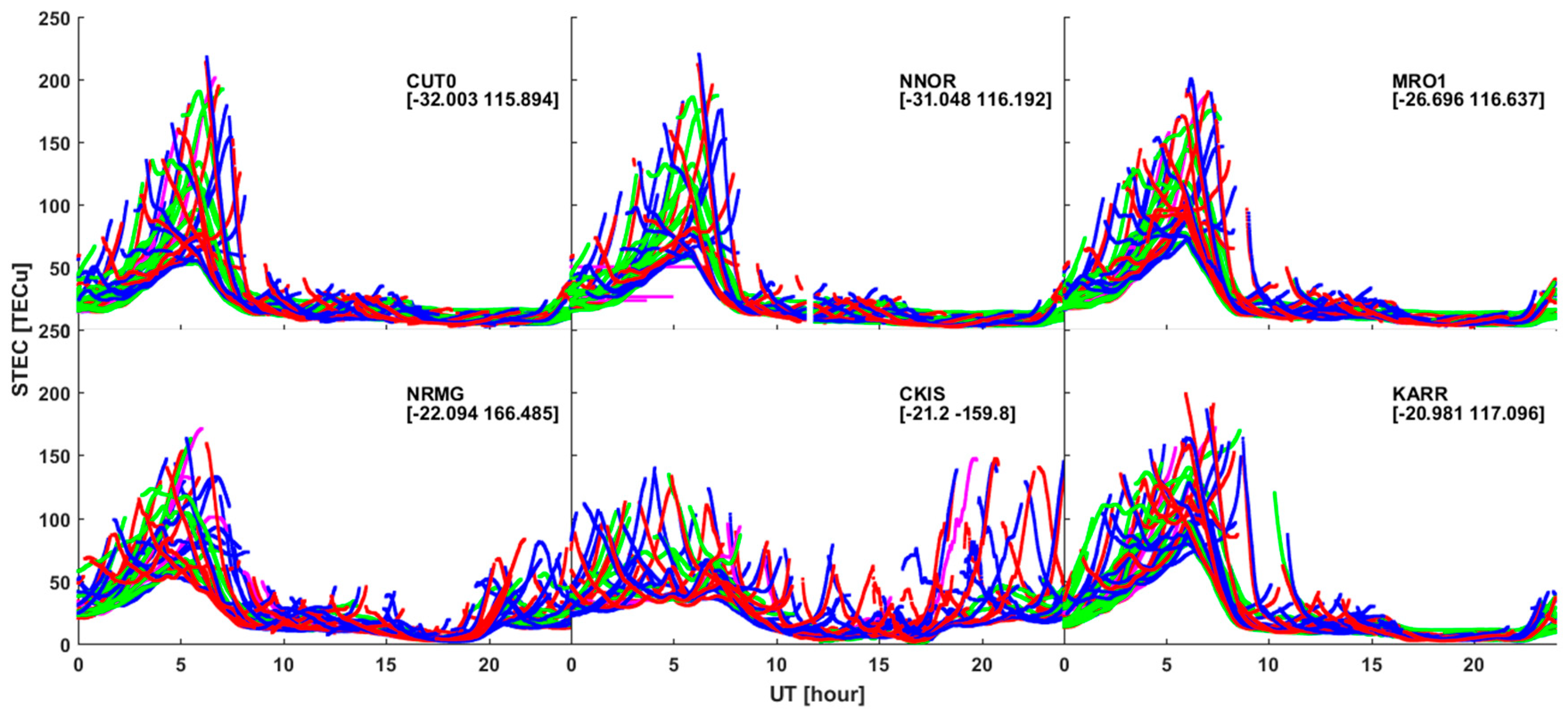
Figure 6.
The vertical TEC (VTEC) responses to the storm at the day of year (doy) 174, 23 June ((a) VTEC; (b) VTEC variation percentage, referred to by Equation (12)).
Figure 6.
The vertical TEC (VTEC) responses to the storm at the day of year (doy) 174, 23 June ((a) VTEC; (b) VTEC variation percentage, referred to by Equation (12)).

Figure 7.
The rate of TEC index (ROTI) observed at high latitudes with MGEX data. (blue: GPS; red: GLONASS; green: BDS; pink: GALILEO).
Figure 7.
The rate of TEC index (ROTI) observed at high latitudes with MGEX data. (blue: GPS; red: GLONASS; green: BDS; pink: GALILEO).

Figure 8.
The spatial characteristics of ROTI derived from the GNSS observables (22–23 June). (a) observed during 20:00–23:00 UT; (b) observed during 03:00–06:00 UT.
Figure 8.
The spatial characteristics of ROTI derived from the GNSS observables (22–23 June). (a) observed during 20:00–23:00 UT; (b) observed during 03:00–06:00 UT.
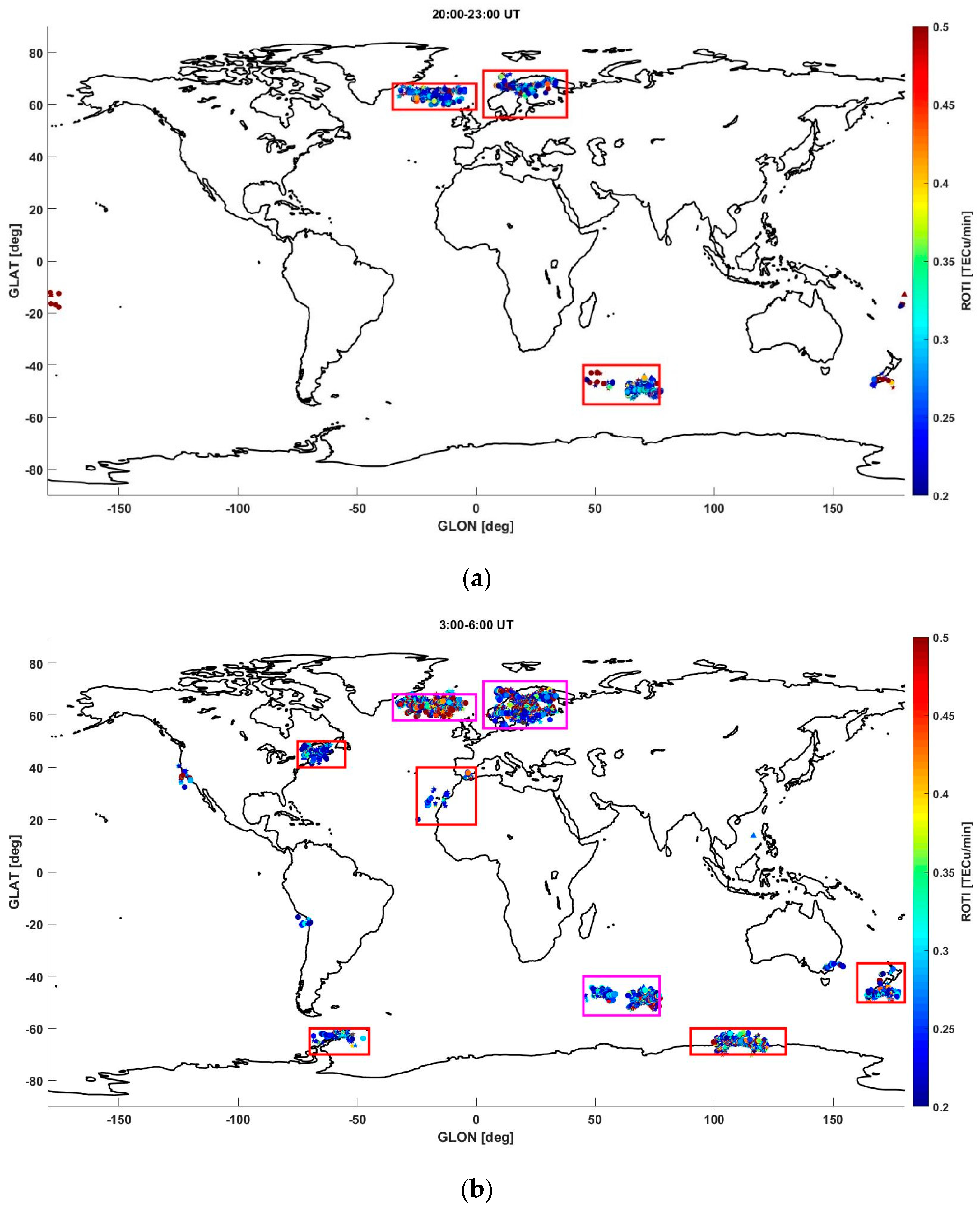
Figure 9.
The prompt penetration electric field from the 22 to 23 June. (yellow padding: first sub-phase storm; light blue padding: second sub-phase storm; red line: PPEF; green line: quiet electric field).
Figure 9.
The prompt penetration electric field from the 22 to 23 June. (yellow padding: first sub-phase storm; light blue padding: second sub-phase storm; red line: PPEF; green line: quiet electric field).

Figure 10.
The ionosphere spatial gradient from the Ous2-Dund sites. (a) doy 156; (b) doy 174.
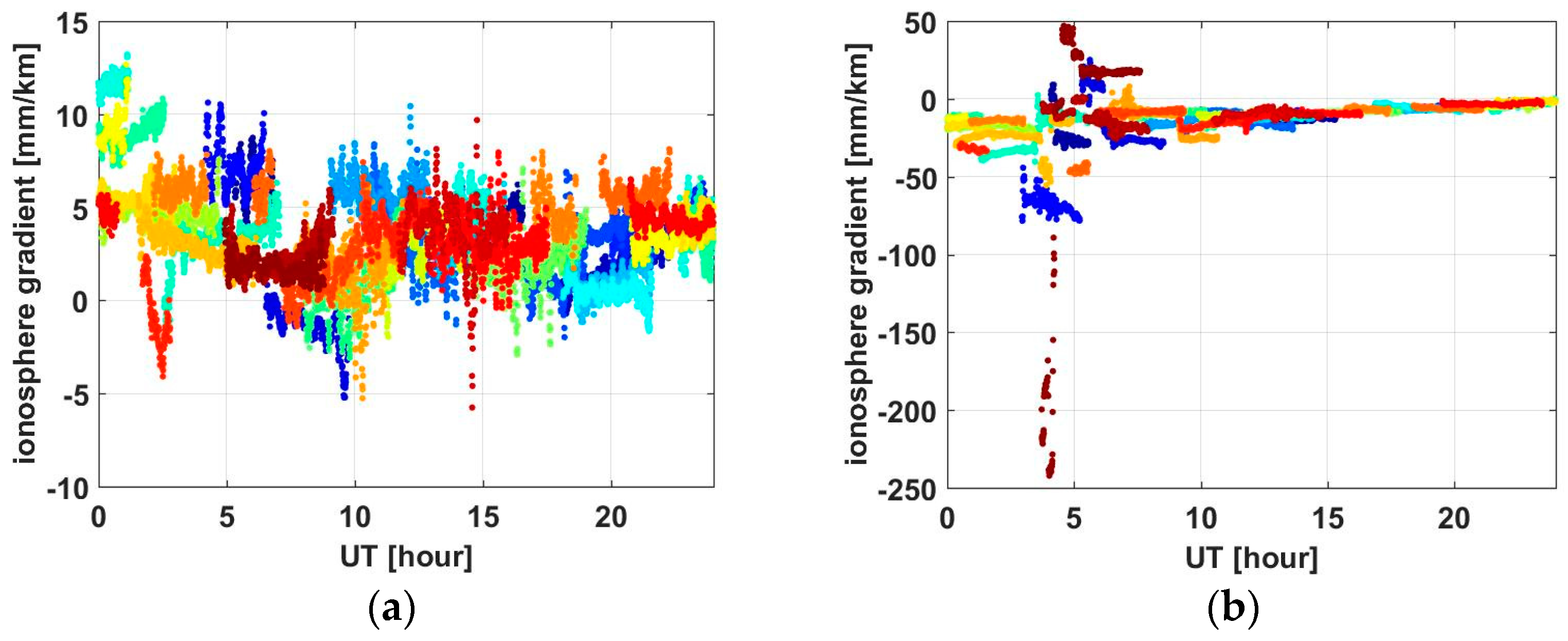
Figure 11.
The ionosphere spatial gradient of satellite PRN32 generated by irregularities.
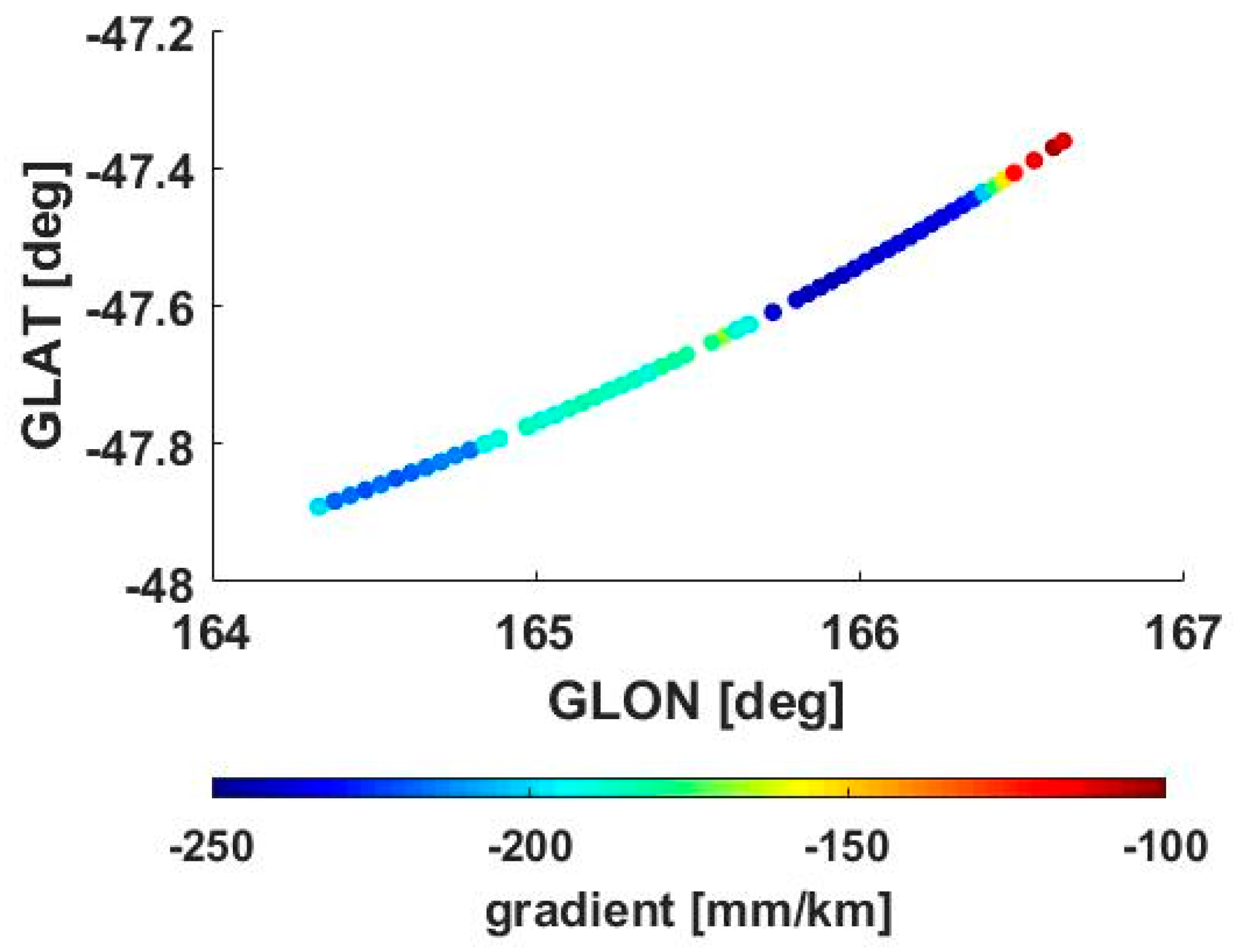
Figure 12.
The ionospheric irregularities evolution with the regional TEC map.

© 2018 by the authors. Licensee MDPI, Basel, Switzerland. This article is an open access article distributed under the terms and conditions of the Creative Commons Attribution (CC BY) license (http://creativecommons.org/licenses/by/4.0/).
Share and Cite
MDPI and ACS Style
Liu, Y.; Fu, L.; Wang, J.; Zhang, C. Studying Ionosphere Responses to a Geomagnetic Storm in June 2015 with Multi-Constellation Observations. Remote Sens. 2018, 10, 666. https://doi.org/10.3390/rs10050666
AMA Style
Liu Y, Fu L, Wang J, Zhang C. Studying Ionosphere Responses to a Geomagnetic Storm in June 2015 with Multi-Constellation Observations. Remote Sensing. 2018; 10(5):666. https://doi.org/10.3390/rs10050666
Chicago/Turabian StyleLiu, Yang, Lianjie Fu, Jinling Wang, and Chunxi Zhang. 2018. "Studying Ionosphere Responses to a Geomagnetic Storm in June 2015 with Multi-Constellation Observations" Remote Sensing 10, no. 5: 666. https://doi.org/10.3390/rs10050666
Note that from the first issue of 2016, this journal uses article numbers instead of page numbers. See further details here.