Assessing Error Correlations in Remote Sensing-Based Estimates of Forest Attributes for Improved Composite Estimation

Abstract

Today, non-expensive remote sensing (RS) data from different sensors and platforms can be obtained at short intervals and be used for assessing several kinds of forest characteristics at the level of plots, stands and landscapes. Methods such as composite estimation and data assimilation can be used for combining the different sources of information to obtain up-to-date and precise estimates of the characteristics of interest. In composite estimation a standard procedure is to assign weights to the different individual estimates inversely proportional to their variance. However, in case the estimates are correlated, the correlations must be considered in assigning weights or otherwise a composite estimator may be inefficient and its variance be underestimated. In this study we assessed the correlation of plot level estimates of forest characteristics from different RS datasets, between assessments using the same type of sensor as well as across different sensors. The RS data evaluated were SPOT-5 multispectral data, 3D airborne laser scanning data, and TanDEM-X interferometric radar data. Studies were made for plot level mean diameter, mean height, and growing stock volume. All data were acquired from a test site dominated by coniferous forest in southern Sweden. We found that the correlation between plot level estimates based on the same type of RS data were positive and strong, whereas the correlations between estimates using different sources of RS data were not as strong, and weaker for mean height than for mean diameter and volume. The implications of such correlations in composite estimation are demonstrated and it is discussed how correlations may affect results from data assimilation procedures.

1. Introduction

Today, remote sensing (RS) data from different sensors and platforms have become increasingly available for estimating forest characteristics at the scale of plots, stands, landscapes, and entire countries or regions, e.g., [1]. For practitioners this development is welcome, but it also poses several challenges with regard to the selection of RS data source for applications. An interesting possibility is to make use of several sources of RS data simultaneously through composite estimation (CE) [2] or in a sequential manner through data assimilation (DA) [3].

An ordinary CE is constructed as a weighted average of several individual estimates; to minimize the variance of the CE, the weights are set inversely proportional to the variance of the individual estimators, e.g., [2]. In case estimates are correlated, this must be taken into account in the calculation of weights and in estimating the variance of the CE. CEs are sometimes applied in national forest inventories, e.g., [4].

DA [3] can be seen as an extension of ordinary CE for the case when time differences between estimates make it necessary to include a model for updating previous estimates to current time before combining with a new estimate. In case the time difference between estimates is short, the difference (in results) between a CE and a standard DA-based estimator, such as the Kalman filter, e.g., [3], is minor. However, DA is a more useful concept than ordinary CE at longer time spans between RS data acquisitions and through DA entire time series of RS data of different kinds can be used for improving the precision of an estimate of current state [5]. Many DA methods exist, e.g., [3], in which the standard Kalman filter assumes independent estimators (or direct observations) at the different time points and a linear model for updating previous estimates to current time. Similarly to ordinary CE, the Kalman filter estimator of current state is a weighted average of a new and an updated estimate; the weights are assigned to be inversely proportional to the variance of the estimators involved.

Studying recent developments in forestry applications of DA, promising results have been obtained in simulation studies [5]. However, the empirical results presented by [6,7] pointed out problems to fully realize the theoretical potential of DA in practice. In the latter studies, making use of only the last measurement for estimating the current state of key forest characteristics was sometimes almost as good as making use of the entire time series through DA. However, all these studies [5,6,7] assumed the estimates to be uncorrelated between subsequent time periods, as is the practice in standard DA through Kalman filtering [3,8,9]. However, using a certain kind of RS data repeatedly, such as data from airborne laser scanning (ALS), e.g., [10], it is likely that certain conditions of a given plot or stand will tend to make the estimates always deviate in a certain direction from the true value. Such conditions could be that a plot is located in steep terrain or that it has an unusual stand structure. Focusing on a specific plot (or stand), such systematic deviations cause biased estimates. However, in applications it will not be known for which plots the estimates tend to be systematically too high or too low, and a reasonable model assumption is that the deviation, based on a certain type of RS data, is composed of two terms: a random effect which remains the same over a certain period of time (due to plot conditions), and a random term which is independent of the other random effect and between subsequent acquisitions (i.e., white noise due to variable RS data acquisition conditions).

Many standard applications of CE and DA assume that the estimates (or observations) are independent. When this is not the case, more advanced methods should preferably be applied but this issue is, sometimes, not fully acknowledged, not even in meteorology where DA has been applied for several decades, e.g., [11], where it is pointed out that treating observations as independent when they are not might lead to substantial loss of DA efficiency.

Although the literature about RS-based assessment of forest characteristics is vast, e.g., [10,12,13,14], no studies appear to be available where error correlations between subsequent estimates are assessed. For ocular stand level inventories, a study of correlated measurement errors was reported by [15].

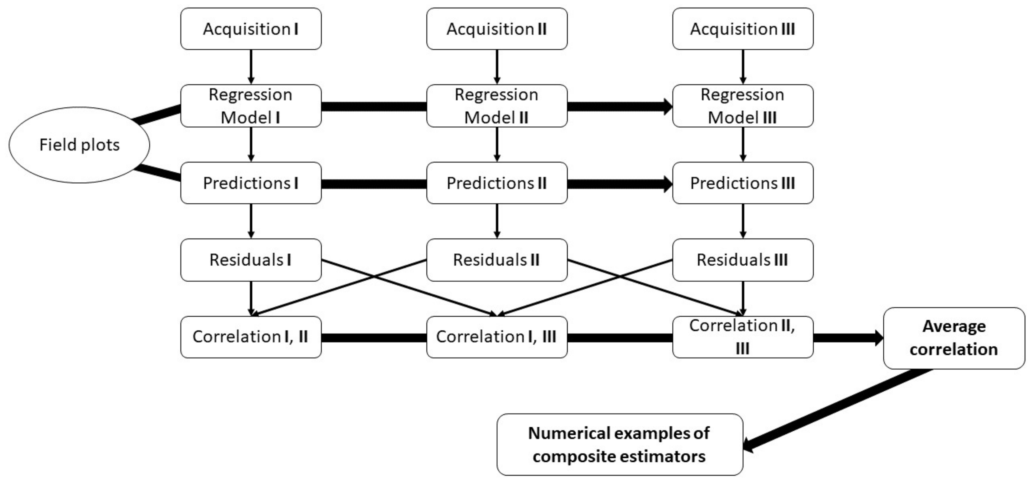
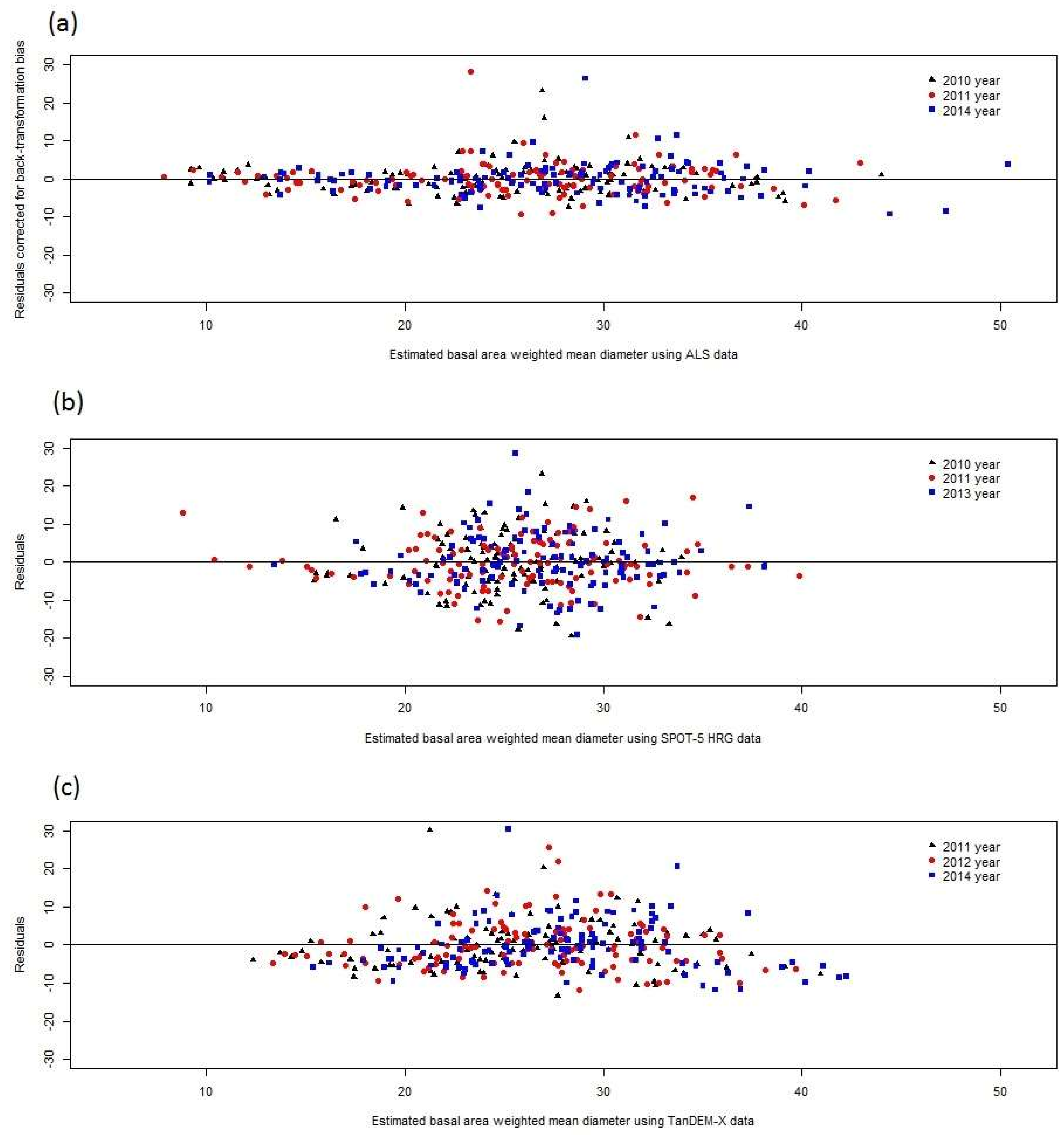
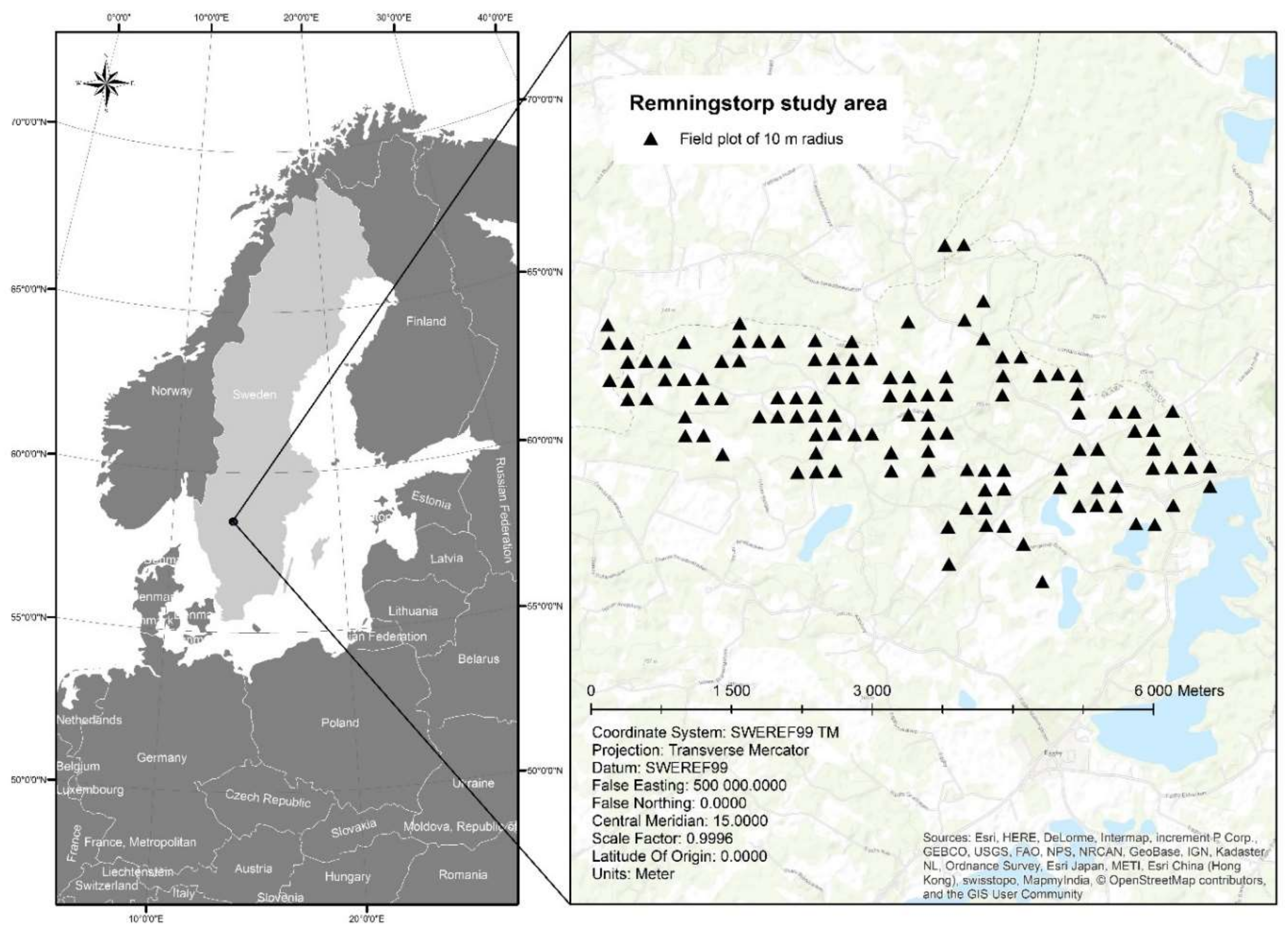
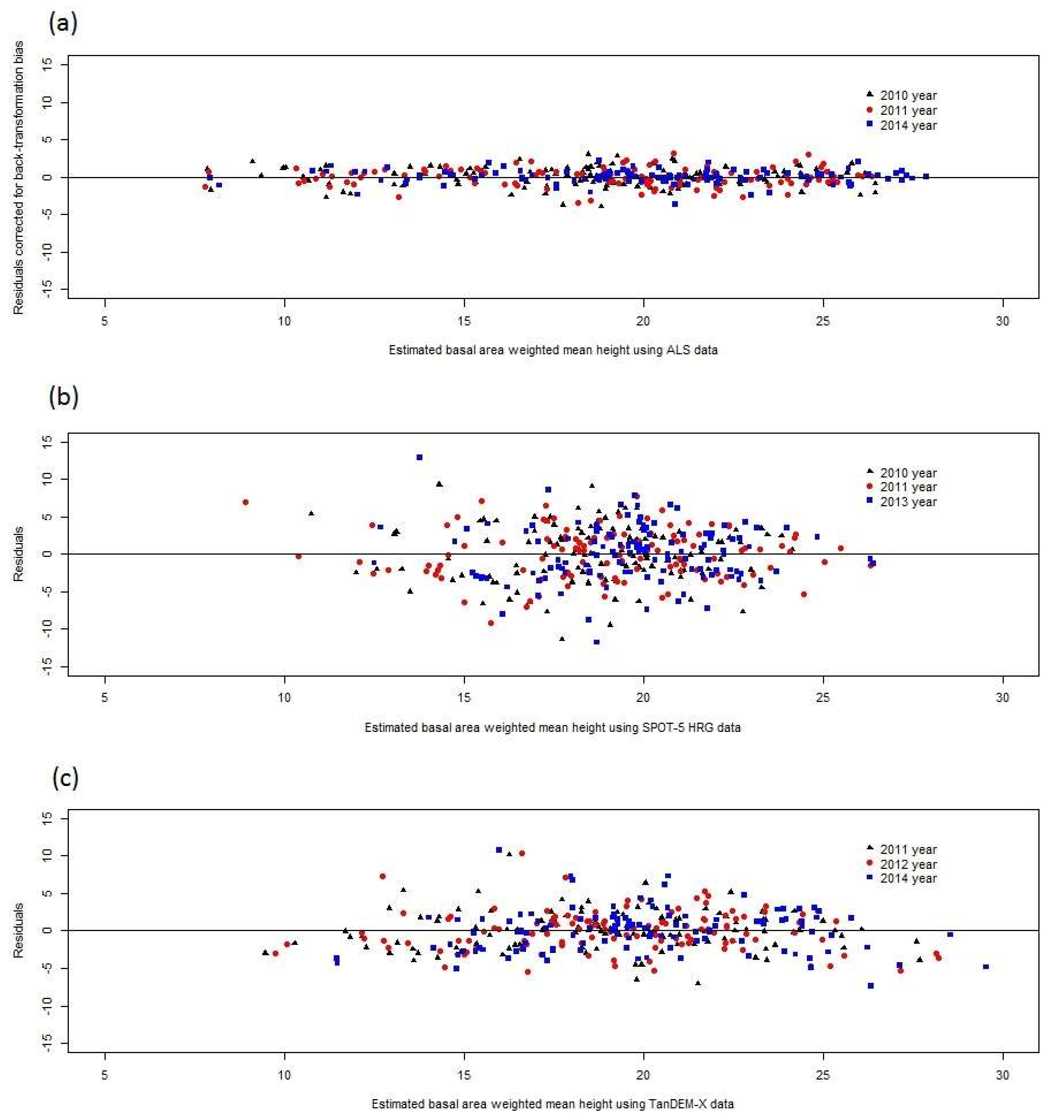
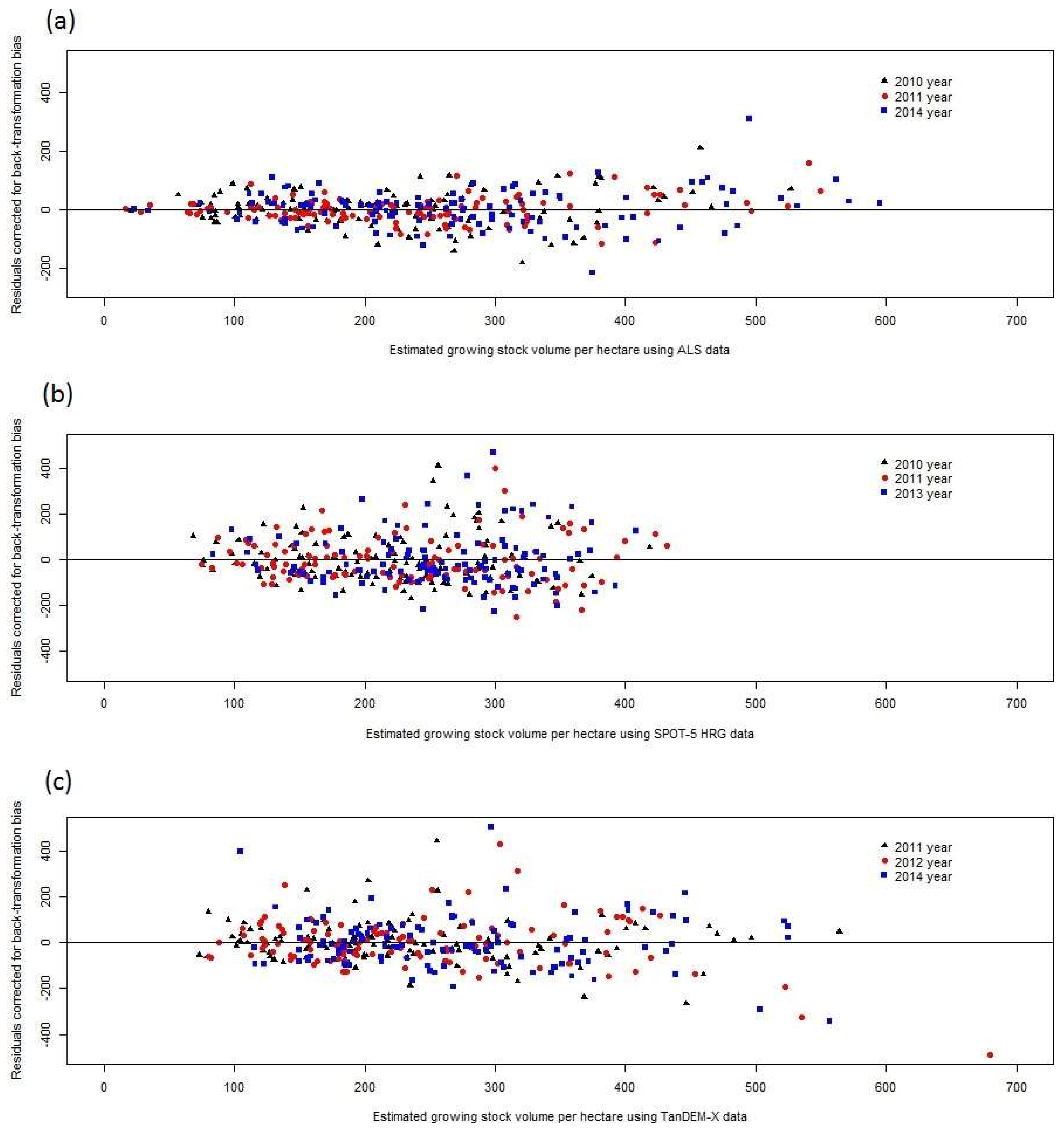
The objective of this study was to estimate the correlation of plot level deviations between estimated and ground truth values, for estimates of forest attributes from different datasets using the same type of RS sensor as well as across estimates using different sensors. The RS data types evaluated were multispectral data from the SPOT-5 satellite, 3D data from airborne laser scanning (ALS), and TerraSAR-X add-on for Digital Elevation Measurement Interferometric Synthetic Aperture Radar (TanDEM-X InSAR) radar data. The forest attributes studied were growing stock volume, basal area weighted mean height (also known as Lorey’s height), and basal area weighted mean diameter. All data were acquired from the Remningstorp test site in southern Sweden. Further, we demonstrate the implication for CE of assuming estimates to be independent in case they are not and we discuss similar implications in DA applications.

As a matter of terminology, we acknowledge the difference between predicting a random variable (e.g., when a regression model is used for predicting an unknown random quantity) and estimating a fixed parameter. However, in order to simplify the text, and since the convention to separate between prediction and estimation seems not to be generally adopted, we have chosen to use the term estimation for both cases [16].

2. Materials and Methods

2.1. Study Area

The study was conducted at the Remningstorp test site in south-western Sweden (Lat. 58°30′N, Long. 13°40′E) (Figure 1). The study area is relatively flat and dominated by Norway spruce (Picea abies) and Scots pine (Pinus sylvestris). For several years, the Remningstorp site has been used for studies of the performance of various types of RS data for forest inventories. Thus, several datasets with RS and field data were available for this study.

2.2. Field Data

Field reference data were acquired at two time-points, during the summers 2010 and 2014. Sample plots with 10 m radius were allocated in a systematic grid across the study area (Figure 1). At both surveys, the diameter of all trees larger than 4 cm at breast height was measured and the species recorded. For a sample of the trees on each plot, additional measurements of height and age were made. Based on these registrations the basal area weighted mean height (Lorey’s height) for a plot was calculated as a weighted average using tree basal area as the weight. The volume of each tree was estimated using the models developed by [17]. The tree level volumes were aggregated and recomputed to correspond to growing stock volume per hectare. The basal area mean diameter was computed for each plot as a standard weighted (by tree basal area) average.

In this study, only plots where no management or other disturbances had occurred during the time period of interest, i.e., between 2010 and 2014, were used. Plots where disturbances due to, e.g., storm or management activities had occurred were identified by comparing the plot level basal area in 2014 with that in 2010. If a decrease was observed the plot was considered disturbed and was discarded from the analysis. Further, plots where the basal area weighted mean age was lower than 20 years in 2014 were excluded since our focus was on middle-aged and old forests. Due to these criteria, 117 of the original 211 plots were left for the analysis (Figure 1).

For each source of RS data and time point of acquisition (see the next section), field data were either forecasted or back-casted a short period of time using linear interpolation, to match the time point of the RS acquisition. Any minor errors caused by the fore- or back-casing were ignored.

Regression analysis, e.g., [18], was applied at the level of sample plots to estimate models with growing stock volume, mean diameter, and mean height as response variables (from field measurements) using RS data as predictor variables.

In

Table 1. Field data statistics for the variables of interest (based on 117 field plots).

Year	Mean Diameter (cm)				Mean Height (m)				Volume (m3 ha−1)
	min	mean	max	sd	min	mean	max	sd	min	mean	max	sd
2010	8.00	25.15	50.10	8.46	6.30	18.67	27.60	4.67	16.40	218.60	667.1	127.05
2014	9.30	27.60	55.50	8.58	7.10	19.99	28.00	4.57	23.30	270.70	803.90	143.88

we present statistics based on the field data collected in 2010 and 2014.

2.3. Remote Sensing Data

Estimates of forest characteristics based on three different kinds of RS data were evaluated in the study. These were ALS data, e.g., [10], TanDEM-X InSAR satellite data, e.g., [19], and multispectral data from the Satellite Pour l’Observation de la Terre 5 High Resolution Geometric (SPOT-5 HRG) sensor, e.g., [20] (Table 2). The RS data were aggregated or resampled to spatial units corresponding to field plots.

2.3.1. ALS Data

Laser scanning data were acquired in 2010, 2011 and 2014. The 2010 data were acquired using a TopEye MK III scanner with wavelength 1550 nm and flown by a helicopter at 400 m.a.g.l. The scan angle was up to 30 degrees and the resulting point density 15 points per m².

The 2011 data were taken from the national laser scanning campaign [21], acquired during leaf off conditions using a Leica ALS60/23 scanner with wavelength 1064 nm and flown at 1700–2300 m.a.g.l. The scan angle was up to 20 degrees and the resulting point density 0.5–1 points per m².

The 2014 data were acquired using a Riegl LMS Q680i scanner with wavelength 1550 nm and flown by a helicopter at approximately 300 m.a.g.l. The scan angle was up to 30 degrees and the average point density 30 points per m².

First returns were used for the digital surface model (DSM) and last returns for the digital elevation model (DEM). The DEM was used to extract the point cloud of returns corresponding to the vegetation, i.e., the digital vegetation model (DVM). An upper threshold of 35 m height was used for the DVM [13]; the lower threshold was 2 m. To compensate for uneven point densities in the different datasets the point cloud was thinned by placing a regular grid with 0.5 by 0.5 m spacing and randomly selecting (maximum) one point within each grid cell to be retained in the DVM. In this study, an area-based estimation approach [10] was used. Points in the DVM within 10 m from the center-coordinate of each plot were extracted and twenty-six ALS metrics were calculated:

• maximum height
• minimum height
• mean height
• standard deviation
• variance
• coefficient of variation
• skewness
• kurtosis (a measure of whether the data are peaked or flat relative to a normal distribution)
• 15 different “height percentiles”, i.e., heights at different percentiles of the DVM
• canopy relief ratio
• percentage of first returns above 2 m as a crown cover estimate

2.3.2. Multispectral SPOT-5 HRG Data

The SPOT-5 HRG multispectral data were acquired at three time-points between 2010 and 2013. Values of four different bands were available: Band 1 which is the green spectral band, Band 2 which is the red spectral band, Band 3 which is the near infrared (NIR) spectral band, and Band 4 which is the short-wave IR spectral band. The spectral reflectance values from all four bands were used as predictor variables in regression modelling of forest attributes as dependent variables. Bands 1–3 have a 10 × 10 m ground sampling distance (GSD), whereas Band 4 has a 20 × 20 m GSD. The weighted mean value function was used to extract spatially interpolated band values for each field plot using the R packages “rgdal” [22] and “raster” [23].

2.3.3. TanDEM-X Data

TanDEM-X InSAR data were selected from three acquisitions between 2011 and 2014, all acquired in stripmap mode. SAR data can be acquired frequently, since they are not dependent on cloud free conditions. The interferometric scattering height (ISH) and the coherence magnitude (COH) were derived using a traditional interferometric processing scheme of the TanDEM-X pairs, as described in [24]. Generated rasters had a 5 × 5 m GSD. The ISH was normalized with a digital elevation model obtained from ALS. Both the normalized ISH and COH have been shown to have a strong correlation with forest attributes in previous studies [7,24,25], and thus both these characteristics were extracted for the field plots with the same procedure as for the SPOT-data.

A summary of the RS data used in the study is given in

Table 2. A summary of the remote sensing (RS) data acquisitions used in the study. ALS: airborne laser scanning.

Year/RS Data Type	ALS	SPOT-5 HRG	TanDEM-X
2010	29 August	4 June	−
2011	4 April	6 June	4 June
2012	−	−	1 June
2013	−	17 July	−
2014	14 September	−	8 June

.

2.4. Methodology

In this section we present the methodological approach of the study. Figure 2 presents an overview.

2.4.1. Regression Analysis

Four different regression model forms were investigated for every RS data type: a linear model, denoted “LINEAR”; a model where both the response variable and the predictor variables were transformed by taking natural logarithms, denoted ‘LOG–LOG’ [18]; a model where only the response variable was transformed by the natural logarithm, denoted ‘SEMILOG’ [18]; and a model where the response variable was transformed by the square root, denoted ‘SQRT’. In selecting the most appropriate model for each RS data type and model form, a forward selection stepwise procedure, cf. [18], in the R package “stats” [26] was applied, using the Akaike information criterion, e.g., [18], for selecting the appropriate number of predictor variables to include in the models. Subsequently, to choose between the four different model forms, residual scatterplots were examined for heteroscedasticity and in case of severe heteroscedasticity (assessed by ocular inspection) the model was abandoned. Remaining models were inspected for outliers and trends in the residuals versus the predictor variables; no such trends were found and no outliers were removed (although the residuals of several observations exceeded two standard deviations). Finally, transformed response variables were back-transformed and corrected for back-transformation bias by multiplication with a factor calculated as the sum of observed values over the sum of back-transformed (non-corrected) estimated values [27], and the model with the smallest root mean square residual error, based on back-transformed values, was selected. Due to the transformations of the response variable, the coefficient of determination (R-squared) was not an appropriate measure for selecting the best model.

Table 3. Regression model forms used in this study.

Variable of Interest	ALS	SPOT-5 HRG	TanDEM-X
Mean diameter (cm)	LOG-LOG	LINEAR	LINEAR
Mean height (m)	SEMILOG	LINEAR	LINEAR
Volume (m3 ha−1)	LOG-LOG	SEMILOG	SEMILOG

presents the selected model forms for each RS data type and each variable of interest. Examples of residual scatterplots (after back-transformation) are shown in Appendix A. Note that all the models provide estimates in “real space”, since in the case of transformations back-transformations were made before the models were applied.

The relative root mean-square errors (RMSEs) in relation to observed values for each RS type of data and variable of interest are given in

Table 4. Relative RMSE (%) for the selected regression models.

Year	Mean Diameter			Mean Height			Volume
	ALS	SPOT-5 HRG	TanDEM-X	ALS	SPOT-5 HRG	TanDEM-X	ALS	SPOT-5 HRG	TanDEM-X
2010	16.67	29.94	−	7.10	20.58	−	27.03	47.10	−
2011	16.90	25.41	24.27	6.39	17.35	13.67	18.82	43.60	39.60
2012	−	−	24.31	−	−	13.97	−	−	44.64
2013	−	26.99	−	−	19.07	−	−	45.90	−
2014	15.53	−	23.68	4.43	−	14.20	23.62	−	41.95

, for the regression models with best fit. The relative RMSE is defined as $100\%\times \frac{\sqrt{\frac{1}{n}{{\displaystyle \sum }}_{i=1}^n{(y_i-{\widehat{y}}_i)}^2}}{\overline{y}}$, with $\overline{y}=\frac{1}{n}{{\displaystyle \sum }}_{i=1}^n{y}_i$, where $y_i$ is the observed value at the ith plot, ${\widehat{y}}_i$ is the corresponding predicted value and n is the number of field plots. In Appendix B, the results for all model types are shown.

It can be observed that the ALS-based models are most precise, and that the estimates based on TanDEM-X are slightly more precise than the estimates based on SPOT data. These findings are consistent with the results of previous studies, e.g., [12,28,29,30].

2.4.2. Correlation between Residuals

As described in the introduction, we assume that the residual deviations from the regression models consist of two components: one random plot effect due to the specific conditions on a plot and one component of white noise, due to variable conditions for the RS acquisitions. The properties of both random components are specific to each source of RS data.

The correlations of residuals, obtained through regression analysis at each acquisition type and time, is the focus of this study. The assumed model, used for description but not for calculating the correlations, is

$${\widehat{y}}_{sit}= y_{it}+ b_{si}+ {\delta }_{sit},$$

(1)

which can be easily obtained from ${\widehat{y}}_{sit}-y_{it}=b_{si}+ {\delta }_{sit}$, where ${\widehat{y}}_{sit}$ is the regression analysis-based estimate of a forest characteristic using RS data type $s$ on plot $i$ at time point $t$, $y_{it}$ is the corresponding value obtained from field measurements, $b_{si}$ is the plot random effect, specific to RS data type $s$, and ${\delta }_{sit}$ is white noise. The expected values of $b$ and $\delta$ are zero and their variances depend on the type of RS sensor used and the general plot and RS acquisition conditions. Thus, the residual error, $r_{sit}$ is

$$r_{sit}= b_{si}+ {\delta }_{sit},$$

(2)

with this model assumption, the $b$-term will make the residuals correlated across time on a given plot (assuming the time period is reasonably short, so that the general plot conditions do not change). The correlation between the residuals from two subsequent estimates for a given plot with the same RS data type will be (assuming $var\left(\delta \right)$ is constant):

$$corr\left(r_{si1}, r_{si2}\right)=\frac{cov\left( r_{si1}, r_{si2} \right)}{\sqrt{var\left(r_{si1}\right) var\left(r_{si2}\right) }}=\frac{var\left(b_{si}\right)}{var\left(b_{si}\right)+var\left({\delta }_{si}\right)}.$$

(3)

To estimate the correlations in Equation (3), pairs of plot level residuals across the 117 plots in Remningstorp were selected. Assuming the variances of the random effects being constant across the different plots, which was supported by fairly homogeneous (back-transformed) residual variances, the correlations were estimated according to the standard formula

$$\widehat{corr}\left({\widehat{r}}_{s1}, {\widehat{r}}_{s2}\right)=\frac{\widehat{cov}\left({\widehat{r}}_{s1}, {\widehat{r}}_{s2}\right)}{\sqrt{\widehat{var}\left({\widehat{r}}_{s1}\right) \widehat{var}\left({\widehat{r}}_{s2}\right) }}.$$

(4)

Here, caps indicate that the quantities were estimated following the regression analysis; e.g., ${\widehat{r}}_{s1}$ is the notation for residuals obtained from the regression analysis based on data at time point 1 from the RS data type $s$. Since three pairs of data were available for a given RS data type and nine pairs for a given combination of two RS data types, the average correlation across all pairs was computed using average covariances and variances in Equation (4) across all three or nine pairs.

Average correlations obtained in this way is the main result of this study. Correlations for all pairs are presented in Appendix C.

2.4.3. Demonstrating the Effect of Correlated Residuals on CE

As pointed out by [11], for meteorological applications, ignoring that measurements (or estimates) are correlated reduces the precision of estimates in DA. Similarly, ignoring that estimates are correlated reduces the potential gains in precision from using CE. In the following we demonstrate the effects of correlated residuals in CE, assumed to be carried out at plot level using several sources of RS data.

The basics of CE are outlined below, in Equations (5)–(7). Denoting two individual estimates by ${\widehat{y}}_1$ and ${\widehat{y}}_2$, the composite estimator is a weighted average, ${\widehat{y}}_{CE}$, i.e.,

$${\widehat{y}}_{CE}= a{\widehat{y}}_1+\left(1-a\right){\widehat{y}}_2.$$

(5)

The weight, $a$, is chosen so that the variance of ${\widehat{y}}_{CE}$ is minimized. The variance is

$$var\left({\widehat{y}}_{CE}\right)= a^{2}var\left({\widehat{y}}_1\right)+{\left(1-a\right)}^{2}var\left({\widehat{y}}_2\right)+2a\left(1-a\right)cov\left({\widehat{y}}_1,{\widehat{y}}_2\right).$$

(6)

The variance minimization can be conducted using standard optimization techniques, leading to the weight

$$a= \frac{var \left({\widehat{y}}_2\right)-cov \left({\widehat{y}}_1,{\widehat{y}}_2\right)}{var \left({\widehat{y}}_1\right)+var \left({\widehat{y}}_2\right)-2cov \left({\widehat{y}}_1,{\widehat{y}}_2\right)}.$$

(7)

This result is often referred to as weighting inversely proportional to the variance, in case covariances are ignored. Composite estimators can be straightforwardly developed for cases with more than two individual estimates. In the general case the weights should be selected as

$$\mathit{w}= \frac{\mathbf{1}}{{\mathbf{1}}_{\mathit{n}}^{\mathit{T}}{\mathit{C}}^{-\mathbf{1}}{1}_{\mathit{n}}}\times {\mathit{C}}^{-\mathbf{1}}{\mathbf{1}}_{\mathit{n}}.$$

(8)

Here, $\mathit{w}$ is the vector of weights for the n individual estimates, C⁻¹ is the inverse of an n × n covariance matrix for the estimators involved, and ${\mathbf{1}}_{\mathit{n}}$ is an n-length vector of unit values.

When many estimates are available for a CE, the most straightforward approach is to apply Equation (8) to obtain all the weights simultaneously. However, an alternative approach is to apply Equations (5)–(7) repeatedly. In this case a first CE is formed from the first two individual estimates, which is then combined with a third individual estimate, etc. Interestingly, this approach to forming a CE resembles DA (using the Kalman filter) for the case where the forecasting step is either non-existing or concerns very short time intervals, so that it can be assumed that the true state remains unchanged.

In the demonstration examples below we have formed CEs in the sequential way in order to show consequences of ignoring correlated residuals and shed light on effects of such simplification in CE and DA applications. The examples are based on assumed correlations which were selected to roughly correspond to the findings in this study. The results are shown in relative terms so that the magnitude of the standard deviation of the residuals is not important for the interpretation of the results.

We demonstrate the consequences of ignoring correlated residuals for the following three cases, denoted A, B and C:

• In a series of 10 RS-based estimates within a short period of time we show the consequences in terms of estimated and true standard deviation of the CE, and the weight assigned to each new estimate, when the same RS data type was used for all 10 estimates assuming:
  • uncorrelated estimates
  • a correlation of 0.4 between the residuals
  • a correlation of 0.8 between the residuals
• In a series of 10 equally precise estimates the first five were obtained using one type of RS data and the last five another type of RS data. We demonstrate the consequences in terms of standard deviation of the CE using weights that either take residual error correlations into account, or assume uncorrelated residuals. We do this for two sub-cases:
  • the error correlation across estimates using the same type of RS data is 0.9 for the first 5 estimates and 0.4 for the last 5 estimates; the correlation of residuals across RS data types was assumed to be 0.2
  • the error correlations for both types of RS data were assumed to be 0.6, and the correlation across RS data types 0.2
  Case B could occur if a certain type of RS data can only be acquired under certain weather conditions (such as optical satellite data), whereas other sensors do not have such limitations (such as radar data).
• After a series of 10 estimates obtained from the same RS data type, an 11th estimate, independent of the first ten, is obtained. Consequences in terms of estimated and true relative standard deviation of the CE after the 11th observation, and the weight assigned to the 11th estimate, are shown, for the cases of accounting for residual error correlations and ignoring them. We assume that the correlation of residuals for the first ten estimates is 0.8 and that the 11th estimate is uncorrelated with the previous estimates and has:
  • 50% standard deviation (compared to of each of the first ten estimates)
  • 100% standard deviation
  • 200% standard deviation

In the computations, we recursively applied Equations (5)–(7) over the series of 10 estimates. After each new estimate, we calculated the variance of the CE, applying Equation (6) with the weight obtained from Equation (7), and used it as the variance of the CE entering the next step. To do this the covariance between the CE and a new estimate must be known. From Equations (1)–(3) it is noted that the correlation between residuals is due to the random plot level effect that remains the same across estimates. In Case A and Case C (up to the 10th estimate) each CE will contain exactly one b_si-component since they are weighted averages of two estimates, each of which contains exactly one b_si-component. Thus, for these cases the covariance was obtained by multiplying the correlation with the variance of the residuals for the given RS data type. Case B is slightly more complicated and in this case there is a need to recursively keep track of what proportion of the CE stems from estimates using the two different RS data types involved. In this case, the covariance will include a component which is due to within-RS data type correlation and another component which is due to across RS data type correlation.

3. Results

3.1. Correlations between and within RS Data Types

The averages correlations of residuals within and between RS data types are given in

Table 5. Average correlation for the residuals of mean diameter.

RS Data Type	ALS	SPOT-5 HRG	TanDEM-X
ALS	0.86	−	−
SPOT-5 HRG	0.53	0.89	−
TanDEM-X	0.63	0.68	0.84

(for mean diameter),

Table 6. Average correlation for the residuals of mean height.

RS Data Type	ALS	SPOT-5 HRG	TanDEM-X
ALS	0.54	−	−
SPOT-5 HRG	0.21	0.84	−
TanDEM-X	0.31	0.43	0.63

(mean height), and

Table 7. Average correlation for the residuals of volume per hectare.

RS Data Type	ALS	SPOT-5 HRG	TanDEM-X
ALS	0.75	−	−
SPOT-5 HRG	0.49	0.91	−
TanDEM-X	0.59	0.59	0.78

(volume per hectare).

It can be noted that all correlations are positive and rather strong. The within-RS sensor correlations are mostly stronger than the across-RS data type correlations. Further, the residuals for growing stock volume and mean diameter have stronger correlations than the residuals for mean height. In Appendix C, the correlations between all pairs of data are shown.

3.2. Demonstrating the Effects of Correlated Residuals

For the calculations, we used the R function datassim() available in the R package “DatAssim” [31]. The package is based on a C++ library for linear algebra developed by [32]. The R function datassim() provides estimates based on Equations (5)–(7).

In Figure 3, the effect of correlated residuals for Case A are shown.

Figure 3 demonstrates the rather dramatic decreased precision of CE at moderate to strong residual error correlation compared to the case of uncorrelated estimates. With uncorrelated estimates, the relative standard deviation after ten sequential CE steps is only 32% of the standard deviation of an individual estimate. With an error correlation of 0.4 the relative standard deviation increases to 68% and with a correlation of 0.8 it increases to 91%, which is a rather modest improvement.

However, in this case, where the same type of RS data is assumed to be used repeatedly, the weights allocated to new predictions are the same regardless of whether correlations are accounted for or not in the calculation of weights. This follows from Equation (7). Also, each observation impacts on the final CE with the weight 0.1 once 10 estimates have been included, which can be observed if the weights are calculated according to Equation (8).

Figure 4 demonstrates Case B, where two different RS data types are applied to obtain a series of 10 estimates. They are used in a block of five estimates with the first RS data type followed by a block of five estimates with the second RS data type.

From Figure 4 it can be seen that the weights differ quite substantially between considering and ignoring correlations in the calculation, but although this is the case the standard deviations of the CE do not vary very much (note that all standard deviations in Figure 4 are estimated correctly, i.e., acknowledging the correlated errors, but the weights are computed in two different ways, i.e., accounting for or ignoring residual error correlation).

In testing other subcases (not presented here), similar results were obtained. Thus, although the weights may vary when correlations are correctly considered, the corresponding (true) standard deviations typically do not increase very much if the weights are calculated without considering the correlations.

In

Table 8. Weight allocated to an 11th independent estimate following 10 correlated (0.8) estimates. In the second and third columns the weights account for correlated errors; in the last two columns error correlations are ignored. “Double” precision of the 11th estimate means 50% standard deviation compared to each of the 10 previous, “same” precision means 100% standard deviation, and “half” means 200%.

Precision	Weight Computed Accounting for Correlations	Standard dev. (%)	Weight Computed without Accounting for Correlations	Standard dev. (%)
Double	0.77	43.8	0.29	65.9
Same	0.45	67.1	0.09	82.6
Half	0.17	82.5	0.02	88.4

, results from Case C are presented, where 10 estimates from a given RS data type are followed by an 11th, independent, estimate. In forestry, this could be that 10 RS-based estimates precede a field-based survey.

From Table 8 it can be observed that residual error correlations in this case have a severely negative effect on how an independent 11th estimate is taken into account in a combined estimator. In all three subcases severely erroneous weights were obtained and, contrary to case B, the erroneous weights also had a severely negative effect on the precision of the CE (after including the 11th estimate).

4. Discussion

The correlations between residuals of RS-based estimates of forest attributes were found to be strong in the Remningstorp study area. Further studies are needed to show if this is the case in other areas as well, but as will be further discussed below, several factors linked to how RS-based estimates are derived make it plausible that similar results would be obtained also in other areas. Thus, CEs using RS-data-based estimates of growing stock volume, mean diameter, and mean height (i.e., the attributes evaluated in this study) ideally should consider that the estimates are correlated or otherwise the results will be less precise and misleading in terms of reported variances (and thus confidence intervals) of the CEs. However, it should be pointed out that in most cases only minor gains in precision would be obtained through correctly considering residual error correlations in determining the weights of the individual estimates in CE. Perhaps more importantly, considering correlations makes estimated variances of CEs realistic, whereas CE variances otherwise might be severely underestimated.

In the methods section of the article, it was pointed out that there are many similarities between a CE obtained in a sequential manner, as in this study, and data assimilation using standard Kalman filter approaches [9]. Since the standard Kalman filter assumes uncorrelated estimates most of the conclusions from this study, with regard to CE, would hold for DA as well, although the forecasting step of DA makes direct comparison difficult.

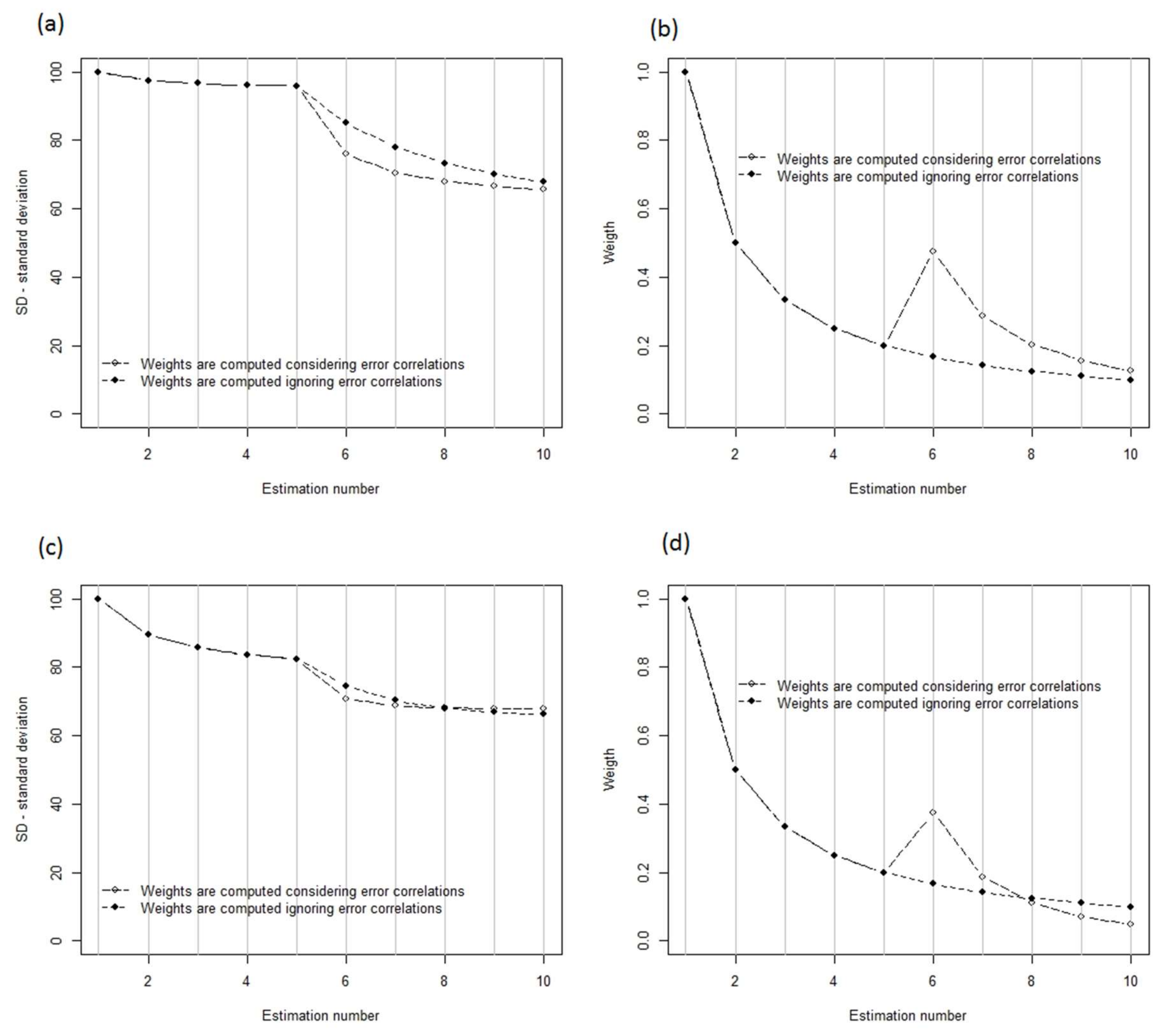
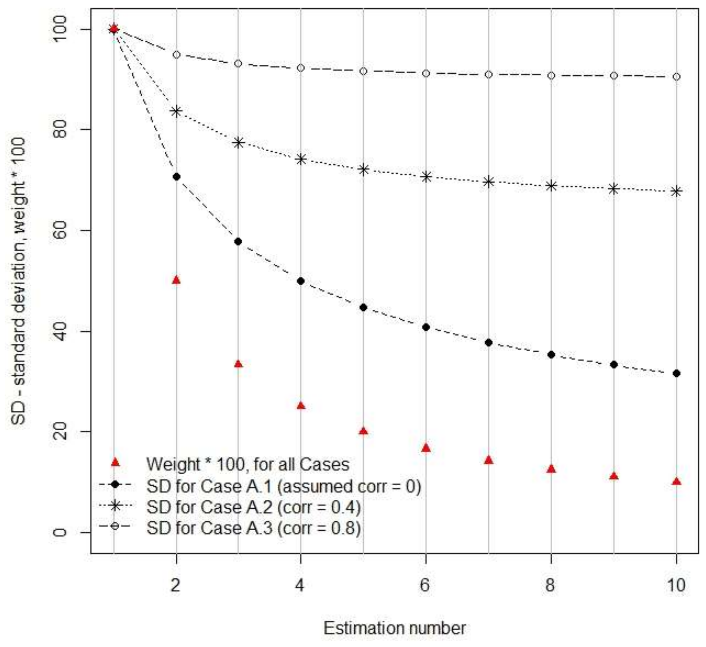
When different types of estimators are mixed in a CE (cases B and C), it was demonstrated that the differences between the estimators, in terms of residual error correlation, must be substantial before the benefit of handling correlations in the computation of weights becomes evident. When the differences, in terms of standard deviation and error correlation, between different RS-data-based estimates were small to moderate (case B) it was found that using slightly incorrect weights did not affect the (true) standard deviation of CE very much. However, with substantial differences between methods (case C) correct handling of error correlations appears to be important. In this case a precise estimate was obtained after a series of correlated, less precise, estimates. The correct solution assigned high weight to the last estimate, and as a result the standard error of the CE was substantially reduced. Ignoring residual error correlation led to a CE with poor, and overestimated, precision.

Strong error correlation might be part of the reason why the empirical studies by [6,7] showed that DA was only slightly better than consistently using only the last RS-data-based estimate. The RS data used in these cases were point clouds from digital aerial photos and TanDEM-X InSAR data, respectively. The first type of data was not evaluated in this study, whereas the latter was found to lead to estimates with substantial error correlations.

Error correlation causes problems also in non-forestry applications of DA, but it appears that it is only rather recently that the topic has been highlighted [11]. In that study, in the context of meteorology, correlated errors obtained from RS data were found to lead to similar problems as the ones identified in this study. In our study all RS data types resulted in moderate to strong error correlations between the regression residuals, across acquisitions using the same sensor. The correlations across RS data types were weaker and this suggests that efficient CE procedures might incorporate estimates from different RS data types, provided the differences in precision are not substantial. However, in doing so the problem observed by [33] must be avoided, i.e., that estimates and estimated variances can be correlated thus causing CEs of the kind applied in this study to be biased. Further, in general the correlations were weaker for height than for volume and diameter, which suggests that CE would work better for this attribute. However, this study was conducted at the level of single plots but in practical forestry estimating attributes at the level of stands is typically more important. Thus, an important continuation of the current study would be to investigate if the plot level effects remain the same within entire stands or if they vary between plots in stands. In the latter case, the potential problems observed in this study would be less severe.

The reasons for the correlated residuals might be several. In general, plots that give a certain response in terms of RS data from a specific sensor still are variable with regard to the target characteristic. For example, plots with the same growing stock volume may have either dense or sparse canopy cover, or they may be located in either steep or flat terrain, leading to different registered reflectance values in a satellite image. This underlies the well-known effect in regression analysis that the estimates “tend towards the mean”, i.e., that the highest true values tends to be underestimated and the lowest true values overestimated.

5. Conclusions

The main conclusion of this study is that it is important to consider regression error correlation between RS-based estimates in composite estimation. Ignoring the correlations might lead to less precise CEs with substantially underestimated variances and, hence, non-trustworthy confidence intervals.

References

1. McRoberts, R.E.; Tomppo, E.O. Remote sensing support for national forest inventories. Remote Sens. Environ. 2007, 110, 412–419. [Google Scholar] [CrossRef]
2. Wolter, K.M. Composite estimation in finite populations. J. Am. Stat. Assoc. 1979, 74, 604–613. [Google Scholar] [CrossRef]
3. Talagrand, O. Data Assimilation: Making Sense of Observations; Springer: Berlin, Germany, 2010. [Google Scholar]
4. Fridman, J.; Holm, S.; Nilsson, M.; Nilsson, P.; Ringvall, A.H.; Ståhl, G. Adapting National Forest Inventories to changing requirements–the case of the Swedish National Forest Inventory at the turn of the 20th century. Silva Fennica 2014, 48, 29. [Google Scholar] [CrossRef]
5. Ehlers, S.; Grafström, A.; Nyström, K.; Olsson, H.; Ståhl, G. Data assimilation in stand-level forest inventories. Can. J. For. Res. 2013, 43, 1104–1113. [Google Scholar] [CrossRef]
6. Nyström, M.; Lindgren, N.; Wallerman, J.; Grafström, A.; Muszta, A.; Nyström, K.; Bohlin, J.; Willén, E.; Fransson, J.E.; Ehlers, S.; et al. Data assimilation in forest inventory: First empirical results. Forests 2015, 6, 4540–4557. [Google Scholar] [CrossRef]
7. Lindgren, N.; Persson, H.J.; Nyström, M.; Nyström, K.; Grafström, A.; Muszta, A.; Willén, E.; Fransson, J.E.S.; Ståhl, G.; Olsson, H. Improved estimation of forest variables using data assimilation of interferometric synthetic aperture radar data. Can. J. Remote Sens. 2017, 43, 374–383. [Google Scholar] [CrossRef]
8. Rabier, F. Overview of global data assimilation developments in numerical weather-prediction centres. Q. J. R. Meteorol. Soc. 2006, 131, 3215–3233. [Google Scholar] [CrossRef]
9. Welch, G.; Bishop, G. An Introduction to the Kalman Filter; TR 95-041; Department of Computer Sciences, University of North Carolina: Chapel Hill, NC, USA, 2006. [Google Scholar]
10. Næsset, E. Predicting forest stand characteristics with airborne scanning laser using a practical two-stage procedure and field data. Remote Sens. Environ. 2002, 80, 88–99. [Google Scholar] [CrossRef]
11. Stewart, L.M.; Dance, S.L.; Nichols, N.K. Correlated observation errors in data assimilation. Int. J. Numer. Methods Fluids 2008, 56, 1521–1527. [Google Scholar] [CrossRef]
12. Næsset, E.; Gobakken, T.; Holmgren, J.; Hyyppä, H.; Hyyppä, J.; Maltamo, M.; Nilsson, M.; Olsson, H.; Persson, Å.; Söderman, U. Laser scanning of forest resources: The Nordic experience. Scand. J. For. Res. 2004, 19, 482–499. [Google Scholar] [CrossRef]
13. Lindberg, E.; Holmgren, J.; Olofsson, K.; Olsson, H. Estimation of stem attributes using a combination of terrestrial and airborne laser scanning. Eur. J. For. Res. 2012, 131, 1917–1931. [Google Scholar] [CrossRef]
14. Saarela, S.; Grafström, A.; Ståhl, G.; Kangas, A.; Holopainen, M.; Nordkvist, K.; Hyyppä, J. Model-assisted estimation of growing stock volume using different combinations of LiDAR and Landsat data as auxiliary information. Remote Sens. Environ. 2015, 158, 431–440. [Google Scholar] [CrossRef]
15. Ståhl, G. A Study of the Quality of Compartment-Wise Forest Data Acquired by Subjective Inventory Methods; Report 24, SLU; Department of Biometry and Forest Management, Swedish University of Agricultural Sciences: Uppsala, Sweden, 1992. (In Swedish) [Google Scholar]
16. Cassel, C.M.; Sarndal, C.E.; Wretman, J.H. Foundations of Inference in Survey Sampling; Willey: New York, NY, USA, 1977. [Google Scholar]
17. Näslund, M. Functions and tables for computing the cubic volume of standing trees. Pine, spruce and birch in southern Sweden and in the whole of Sweden. Rep. For. Res. Inst. Swed. 1947, 36, 68. [Google Scholar]
18. Chatterjee, S.; Simonoff, J.S. Handbook of Regression Analysis; John Wiley & Sons: Hoboken, NJ, USA, 2013. [Google Scholar]
19. Krieger, G.; Moreira, A.; Fiedler, H.; Hajnsek, I.; Werner, M.; Younis, M.; Zink, M. TanDEM-X: A satellite formation for high-resolution SAR interferometry. IEEE Trans. Geosci. Remote Sens. 2007, 45, 3317–3341. [Google Scholar] [CrossRef] [Green Version]
20. Wolter, P.T.; Townsend, P.A.; Sturtevant, B.R. Estimation of forest structural parameters using 5 and 10 meter SPOT-5 satellite data. Remote Sens. Environ. 2009, 113, 2019–2036. [Google Scholar] [CrossRef]
21. Klang, D.; Burman, H.; Digpro, A.B. Airborne Laser Scanning, an Efficient Revision Procedure for the Swedish Digital Elevation Model. In Proceedings of the 7th International Conference on Transparent Optical Networks, Barcelona, Catalonia, Spain, 7 July 2005; p. 10. [Google Scholar]
22. Bivand, R.; Keitt, T.; Rowlingson, B. rgdal: Bindings for the Geospatial Data Abstraction Library, R Package version 1.1-8; 2016. Available online: http://CRAN.R-project.org/package=rgdal (accessed on 3 May 2017).
23. Hijmans, R.J. raster: Geographic Data Analysis and Modeling, R package version 2.5-2; 2015. Available online: http://CRAN.R-project.org/package=raster (accessed on 3 May 2017).
24. Persson, H.J.; Fransson, J.E.S. Comparison between TanDEM-X and ALS based estimation of above ground biomass and tree height in boreal forests. Scand. J. For. Res. 2017, 32, 306–319. [Google Scholar] [CrossRef]
25. Treuhaft, R.N.; Siqueira, P.R. The calculated performance of forest structure and biomass estimates from interferometric radar. Waves Random Media 2004, 14, 345–358. [Google Scholar] [CrossRef]
26. R Core Team. R: A language and Environment for Statistical Computing; R Foundation for Statistical Computing: Vienna, Austria, 2014; Available online: http://www.R-project.org/.
27. Snowdon, P. A ratio estimator for bias correction in logarithmic regressions. Can. J. For. Res. 1991, 21, 720–724. [Google Scholar] [CrossRef]
28. Rahlf, J.; Breidenbach, J.; Solberg, S.; Næsset, E.; Astrup, R. Comparision of four types of 3D data for timber volume estimation. Remote Sens. Environ. 2014, 155, 325–333. [Google Scholar] [CrossRef]
29. Yu, X.; Hyyppä, J.; Karjalainen, M.; Nurminen, K.; Karila, K.; Vastaranta, M.; Kankare, V.; Kaartinen, H.; Holopainen, M.; Honkavaara, E.; et al. Comparison of laser and stereo optical SAR and InSAR point clouds from air-and space borne sources in the retrieval of forest inventory attributes. Remote Sens. 2015, 7, 15933–15954. [Google Scholar] [CrossRef]
30. Hyyppä, J.; Hyyppä, H.; Inkinen, M.; Engdahl, M.; Linko, S.; Zhu, Y.-H. Accuracy comaprision of various remote sensing data sources in the retrieval of forest stand attributes. For. Ecol. Manag. 2000, 128, 109–120. [Google Scholar] [CrossRef]
31. Saarela, S.; Grafström, A. DatAssim: Data Assimilation, R package version 1.0; 2017. Available online: https://CRAN.R-project.org/package=DatAssim (accessed on 10 June 2017).
32. Sanderson, C.; Curtin, R. Armadillo: A template-based C++ library for linear algebra. J. Open Source Softw. 2016, 1, 1–26. [Google Scholar] [CrossRef]
33. Grafström, A.; Ekström, M.; Jonsson, B.G.; Esseen, P.-A.; Ståhl, G. On combining independent probability samples. Surv. Methodol. 2017. Accepted. [Google Scholar]
Figure 1. Overview of the Remningstorp test site in southern Sweden. The location of the 10 m radius sample plots which were used in the study are marked with black triangles.
Remotesensing 10 00667 g001
Figure 2. A flowchart overview of the methods applied in the study.
Remotesensing 10 00667 g002
Figure 3. Demonstration of Case A in terms of relative standard deviation of a composite estimation (CE), making use of 1–10 estimates sequentially assuming different residual error correlations. The weights are the same for all subcases, and shown as red triangles; the values of the weights are scaled by a factor of 100.
Remotesensing 10 00667 g003
Figure 4. Demonstration of Case B in terms of true relative standard deviation on the left side panels (a) and (c), and corresponding weights on the right side panels (b) and (d); for subcase (1) where five estimates with error correlation 0.9 are followed by five estimates with error correlation 0.4 ((a) and (b)); and subcase (2) where five estimates with error correlation 0.6 is followed by five estimates with the same error correlation 0.6 ((c) and (d)).
Remotesensing 10 00667 g004