Observed High-Latitude Precipitation Amount and Pattern and CMIP5 Model Projections

1
Department of Hydrology and Atmospheric Sciences, University of Arizona, 1133 E. James E Rogers Way, Harshbarger, Tucson, AZ 85721, USA
2
Jet Propulsion Laboratory, California Institute of Technology, 4800 Oak Grove Drive, MS 233-300, Pasadena, CA 91109, USA
3
Joint Institute for Regional Earth System Science and Engineering, University of California, Los Angeles, CA 90095, USA
*
Author to whom correspondence should be addressed.
Remote Sens. 2018, 10(10), 1583; https://doi.org/10.3390/rs10101583
Submission received: 3 August 2018
/
Revised: 21 September 2018
/
Accepted: 24 September 2018
/
Published: 1 October 2018
(This article belongs to the Special Issue Remote Sensing of Precipitation)
Abstract
:Utilizing reanalysis and high sensitivity W-band radar observations from CloudSat, this study assesses simulated high-latitude (55–82.5°) precipitation and its future changes under the RCP8.5 global warming scenario. A subset of models was selected based on the smallest discrepancy relative to CloudSat and ERA-I reanalysis using a combined ranking for bias and spatial root mean square error (RMSE). After accounting for uncertainties introduced by internal variability due to CloudSat’s limited four year day-night observation period, RMSE provides greater discrimination between the models than a typical mean state bias criterion. Over 1976–2005 to 2071–2100, colder months experience larger fractional modelled precipitation increases than warmer months, and the observation-constrained models generally report a larger response than the full ensemble. For everywhere except the Southern Hemisphere (SH55, for 55–82.5°S) ocean, the selected models show greater warming than the model ensemble while their hydrological sensitivity (fractional precipitation change with temperature) is indistinguishable from the full ensemble relationship. This indicates that local thermodynamic effects explain much of the net high-latitude precipitation change. For the SH ocean, the models that perform best in the present climate show near-median warming but greater precipitation increase, implying a detectable contribution from processes other than local thermodynamic changes. A Taylor diagram analysis of the full CMIP5 ensemble finds that the Northern Hemisphere (NH55) and SH55 land areas follow a “wet get wetter” paradigm. The SH55 land areas show stable spatial correlations between the simulated present and future climate, indicative of small changes in the spatial pattern, but this is not true of NH55 land. This shows changes in the spatial pattern of precipitation changes through time as well as the differences in precipitation between wet and dry regions.
1. Introduction
Warming in high latitudes is faster than in lower latitudes partly due to meridional heat transport and positive snow/ice-albedo feedback [1,2]. In the Northern Hemisphere, rapid reductions in snow cover, sea-ice extent [3], and thawing permafrost [4] have been observed and an intensification of the hydrological cycle is expected [5]. Warming has also increased sea level through terrestrial ice and glacier loss, but this can be locally mitigated by an increase in snowfall in regions that remain below freezing even under warming [6,7], meaning that understanding high-latitude precipitation is important for calculations of future global-scale risks.
Climate models are key to understanding future precipitation changes but produce a wide range of values, especially on regional scales [8]. Meanwhile, precipitation observations show large spread, especially in high latitudes (e.g., [9]), which is related to limitations in sensors, retrieval techniques, poor understanding of precipitation microphysics, unknown surface emissivity (i.e., over snow and ice), and difficulties in distinguishing between light rain and cloud [10,11]. In recent years, advanced sensors such as CloudSat (Stephens et al., 2008) have improved our quantification of the amount and distribution of high-latitude precipitation. CloudSat has high sensitivity to detect light rainfall and snowfall, two major types of precipitation in high latitudes. Behrangi et al. [12] performed a comparative analysis between CloudSat total precipitation estimates and other products for the regions 55–82.5°S/N (henceforth “SH55” and “NH55”, the polar limit is based on the CloudSat orbit on a 2.5° × 2.5° latitude-longitude grid). The products used were the monthly Global Precipitation Climatology Project (GPCP) V2.3 [13,14], Global Precipitation Climatology Centre (GPCC) full data reanalysis V7 [15], National Centers for Environmental Prediction–Department of Energy Reanalysis 2 (NCEP-DOE R2) [16], ERA-interim [17], and Modern Era Retrospective-Analysis for Research and Applications (MERRA) [18,19]. Mean precipitation and spatial statistics showed that both ERA-I and GPCP generally agreed well with CloudSat, although CloudSat does not have a formal rainfall product over land and so it was not considered robust over NH55 land. One area of disagreement was winter precipitation over northern Eurasia, where GPCP was a high outlier relative to the other non-CloudSat products, and where independent GRACE data did not show a mass increase consistent with GPCP accumulations.
Here our objective is to use the updated understanding of precipitation over SH55 and NH55 land and ocean from Behrangi et al. [12] to assess model performance and determine how current understanding of the amount and spatial distribution of high-latitude precipitation can be used to add insights onto projected future changes in precipitation under global warming. Other studies have assessed how Coupled Model Intercomparison Project, phase 5 (CMIP5) models simulate precipitation (e.g., [20,21,22]), but here we specifically consider higher latitudes.
One approach to potentially narrow ranges in climate projections is to sub-select models based on how well they simulate properties or processes in the current climate. One example of this approach is that of “emergent constraints” in research related to climate or hydrological sensitivity [23]. With regards to precipitation, Palerme et al. [24] compared CloudSat snowfall with that of CMIP5 models over Antarctica and identified that sea-ice extent is a key predictor of simulated Antarctic snowfall. They also considered a subset of CMIP5 models whose mean Antarctic precipitation was within ±20% of that from the CloudSat 2C-SNOW product. Here we consider land and ocean in both hemispheres, rather than just Antarctica, and assess whether the observation-based spatial pattern of precipitation can be used as an additional constraint to reduce the modelled spread of future high-latitude changes.
The use of spatial distribution of precipitation in principle means that greater information can be extracted from a relatively short period, such as the 4 full years for which CloudSat operated both day and night. Some previous studies (i.e., [25]) have found a dominant role of bias in determining model skill scores. We find that models disagree more strongly in terms of their simulated spatial pattern of precipitation than in terms of their means, relative to the uncertainties introduced over a 4-year period by internal variability. This indicates that additional use of spatial information provides a more robust method for ranking models by performance and determining whether better performing models indicate different future changes.
2. Dataset
Building on Behrangi et al. [12], we select reference observation datasets as follows: (1) CloudSat for rain and snowfall over ocean and precipitation over Antarctica where snowfall accounts for 99% of total precipitation, and (2) ERA-interim (here after ERA-I) over Northern Hemisphere land where rainfall is a major contributor and a reliable CloudSat retrieval is not available. Note that while GPCP showed similar agreement with CloudSat for Antarctic precipitation, several studies suggest that GPCP over estimates precipitation in parts of Eurasia, which may be related to biases in the correction for gauge undercatch. We selected ERA-I as it was more consistent compared to CloudSat over both NH55 ocean and SH55 land and ocean. Data were mapped onto a 2.5° × 2.5° latitude-longitude grid, which allows sufficient CloudSat samples to stabilize grid-box-level statistics.
2.1. CloudSat
Due to its high sensitivity to light rain and snowfall, which occur frequently in high latitudes, CloudSat has been widely used in analysis of high latitude precipitation [26,27,28,29]. This is particularly important due to the sparseness of stations and inherent limitations of other satellite-based precipitation estimates in high latitudes [26,27]. Three CloudSat products are used here: 2C-PRECIP-COLUMN R04 (henceforth “2c-column”; [30]), 2C-RAIN-PROFILE R04 (henceforth “2c-rain”) [11], and 2C-SNOW-PROFILE (henceforth “2c-snow”) [31] along with the CloudSat auxiliary AMSR-E product CS_AMSRE-AUX (henceforth “AMSR-E”). All data are available at: http://www.cloudsat.cira.colostate.edu. 2c-column provides precipitation occurrence, phase (rain, snow or mixed), and likelihood (certain, probable, possible). We restrict our analysis to “certain” for all phases. Non-certain events tend to be of low intensity and in the case of 2c-snow, including non-certain events only increases mean snowfall rate in the SH55 region by +2.9% and in the NH55 region by +4.5%.
It should be noted that while CloudSat provides a viable source for precipition estimation in high latitudes, it may also face some limitations. In very intense rain the radar signal is saturated and the CloudSat algorithm may provide a lower limit on the rain intensity. This may limit the ability of CloudSat at the higher end of snowfall intensity distribution [32,33]. Signal saturation is often infrequent in high latitudes (especially poleward of latitude 60° [26]), but when it does, coincident AMSR-E estimates from CS_AMSRE-AUX can be used similar to Behrangi et al. [26]. Addition of AMSR-E is particularly effective over ocean where AMSR-E precipition retrievals are based on both emission and scattering signals. Accordingly, the CloudSat estimates used in the present study employs AMSR-E data when signal saturation is noted. CloudSat may also miss shallow precipitation. In CloudSat product, near surface precipitation is estimated at about 1.0 km above the ocean surface (and ~1.5 km over land) to avoid contamination of the reflectivity profile by surface returns [34] that can result in missing shallow precipitation. This limitation has been shown by comparing CloudSat estimates with ground stations and radars (e.g., [32]), although as stated by the authors identifying a reliable ground truth for evaluation of light-snowfall events is difficult. In another study over Antarctica, it was shown that near surface sublimation of snowfall could be large thus CloudSat precipitation estimates at about 1.5 km over land might produce larger rates than what is observed on ground, mitigating part of the missed shallow precipitation by CloudSat [35].
CloudSat products are available from the summer of 2006 but battery problems forced daylight-only operation since April 2011. As in Behrangi et al. [12], we use the complete years 2007–2010 inclusive.
2.2. ERA-Interim
ERA-interim [16] is a European Center for Medium-Range Weather Forecasts (ECMWF) global atmospheric reanalysis that uses a 4D-VAR scheme to assimilate observations from radiosondes, commercial aircraft, and satellites in a numerical model. Precipitation data are not directly incorporated. This study uses daily precipitation from http://apps.ecmwf.int/datasets/ at 2.5° × 2.5° spatial resolution. Previous evaluation has shown good performance of ERA-I in various high-latitude locations. For example, Medley et al. [36] showed that ERA-I’s mean snow accumulation was within approximately 1σ of airborne radar observations over Thwaites Glacier in West Antarctica. Other work suggests that ERA-I likely more realistically depicts precipitation changes in Antarctica [37] and high-latitude precipitation amount [12] compared to several other reanalyses. The choice ERA-I over NH55 land is mainly based on Behrangi et al. [12] which highlighted potential errors such as gauge undercatch issues in GPCP and GPCC, and the lack of reliable CloudSat rain retrievals over land. Nevertheless, we recognize that the use of ERA-I is also not ideal as ERA-I and CMIP5 models could potentially share similar parameterizations.
2.3. CMIP5 Models
We used output from the 36 CMIP5 climate models listed in Table 1. From the middle of the nineteenth century to 2005, the models are forced by known solar output and atmospheric composition, this is the “historical” experiment [38]. From 2005 until the end of the 21st century, the models are forced under a scenario of high emissions called Representative Concentration Pathway 8.5 (RCP8.5, [39]). This choice is not a statement about the likelihood of RCP 8.5 over other potential pathways, but as it provides a forcing that is both credible and large, giving a larger signal-to-noise ratio for interpreting forced response. After assessing the general high-latitude performance of the models we sub-select 5 for each region (SH55 and NH55 land and ocean, plus Greenland) based on their combined performance in terms of spatial RMSE and mean bias relative to the observation-based product. SH55 land corresponds to Antarctica, and Greenland is separated from the rest of NH55 land for two main reasons. Firstly, it is a unique measurement challenge with its perennial ice and snow cover and poor gauge coverage. Secondly, its potential contribution to sea level change is of great interest and is the focus of an active research community. We therefore separate Greenland to avoid cross-contamination of region-specific errors with other NH55 land, and to provide more easily applied information for ice sheet modelers and sea level rise specialists. The selection methodology is described in Section 3.
2.4. Other Datasets
The present work also uses precipitation data from GPCP, GPCC, MERRA, and NCEP-DOE R2. GPCP is a merged product using data from gauges over land and from satellite over both land and ocean. We used the latest version of the monthly 2.5° × 2.5° resolution GPCP product (version 2.3; [12]). GPCC integrates a large pool of station data from various networks, organizations, and additional resources under support of WMO and produces gridded products at a range of spatial resolutions at daily and monthly time scales [14]. Here we used GPCC Full Data Reanalysis version 7.0 at 2.5° × 2.5° resolution. MERRA [18] uses the Goddard Earth Observing System Data Assimilation System version 5 and assimilates observations for the retrospective analyses. Here we used monthly MERRA V5.2 with 0.66° longitude × 0.50° latitude resolution. The NCEP-DOE R2 product [15] is an improved version of the NCEP product and includes fixed errors and updated parameterizations of physical processes. We used monthly data at T62 spatial resolution (~1.875° × 1.875°).
3. Method
Model ensembles such as CMIP5 are often used to characterise potential future climate change, although as an ensemble of opportunity, CMIP5 cannot be used to calculate formal errors. However, investigating its simulation of the present day climate may reveal model-observation discrepancies that indicate poor model performance and it may also be possible to reduce the range of projections through observation-based constraints that exclude poorly performing models.
Here we investigate the CMIP5 ensemble simulation of high-latitude precipitation based on the observation-based product selection justified in Behrangi et al. [12], and then consider whether the present day simulation of high-latitude precipitation is informative regarding future changes within the ensemble. We do so by selecting models that show the smallest discrepancy relative to CloudSat and ERA-I in both the total amount and spatial distribution of high-latitude precipitation. However, the observational data choice, model selection criteria, and the number of models to include in this subset are subjective. Palerme et al. [24] selected models with a mean discrepancy in mean Antarctic precipitation of ±20% versus CloudSat 2C-snow. Here we include spatial information by using centered and area-weighted RMSE as well as bias. All models are ranked separately for each of SH55 and NH55 land and ocean, and for Greenland, and those within the five lowest sum of rankings for bias + RMSE are used in our primary analysis. Table 1 lists all 36 models used along with labels for those which were within the top 5 rankings for bias, RMSE or bias + RMSE. In many cases a model that is selected based on bias is also picked in the RMSE ranking, but this is not always the case. We present results for both the full ensemble and our 5-member subset, and to address potential sensitivities of our method we also show some results when selecting on bias alone.
While CloudSat provides advanced precipitation data to evaluate the models, only 2007–2010 provide full day-night coverage. For all other datasets we use 1986–2005 which raises questions about the stability and reliability of our rankings. We address this by using GPCP as a test of variability introduced by sub-selecting smaller time periods by comparing 4-year statistics with the values inferred over 1990–2010. This comparison includes the CloudSat period and is of the same length as the other periods used. A further advantage of the later selection is to avoid discontinuities early in the GPCP record, where our analysis shows a larger disagreement in spatial pattern between pre-1990 and later years. These larger changes are more likely to be due to discontinuities introduced by changes in data sources rather than real changes in precipitation distribution.
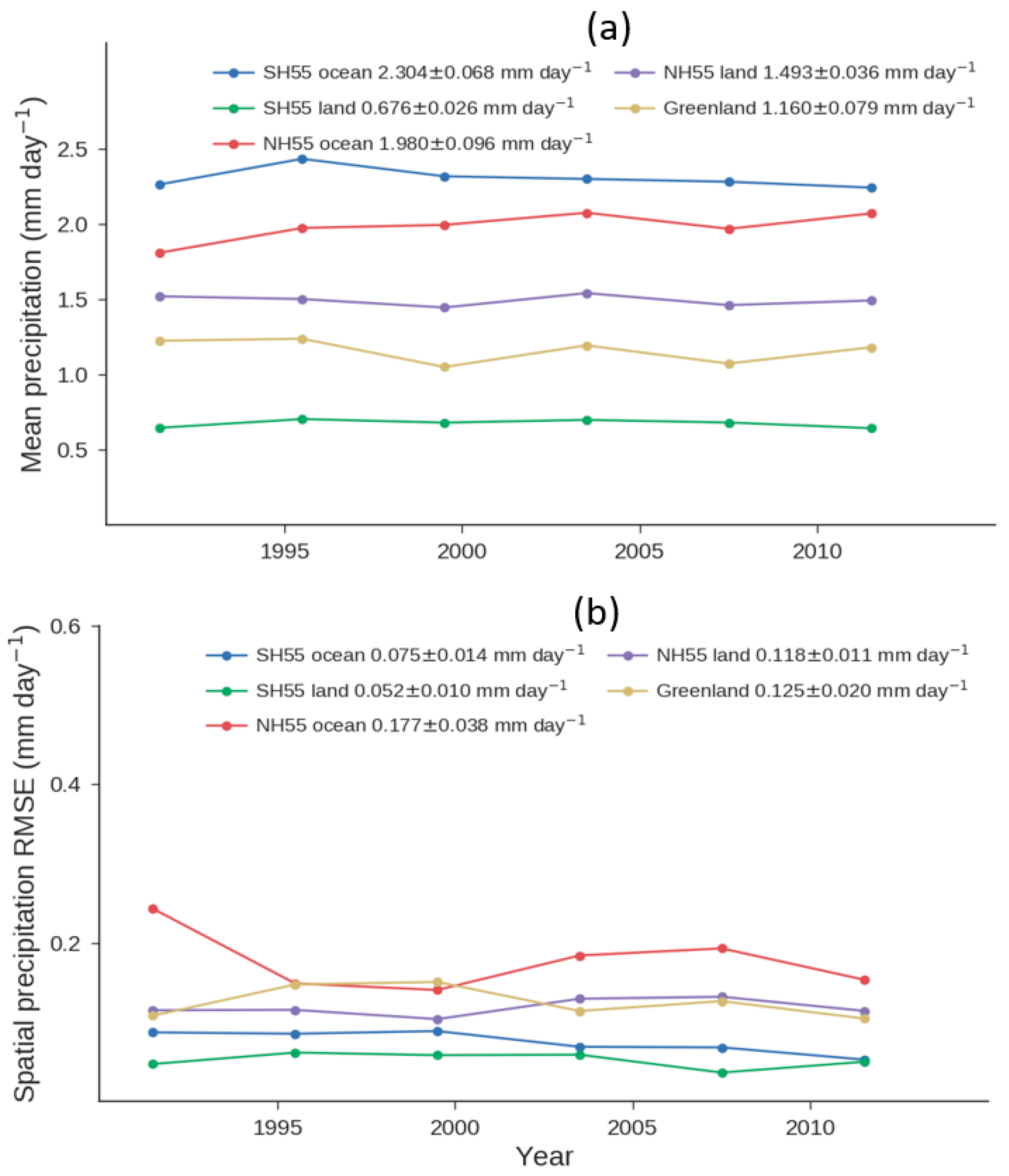
We calculate running 4-year means and RMSEs relative to the 1990–2010 mean pattern for each region and the time series of these statistics are shown in Figure 1. These represent an estimate of the variance introduced due to selecting a four year period compared with the 21-year periods used in our other comparisons.
The standard deviation of the 4-year mean precipitation values provides an estimate of uncertainty in the bias due to the limit of a 4-year CloudSat period whereas the mean value of the RMSE is an estimate of the uncertainty in the RMSE statistic. The variation in the mean precipitation over the oceans and Greenland is similar to the threshold bias used for selecting the top 5 models, indicating that this short time period does not provide a particularly useful constraint on the CMIP5 models. However, the mean RMSE statistic is consistently smaller than that which occurs when comparing CMIP5 simulations with CloudSat. For example, the mean RMSE over SH55 oceans is 0.08 mm day−1, compared with CMIP5 simulations which range from 0.41 to 0.61 mm day−1. Meanwhile, over NH55 oceans the 4-year CloudSat RMSE is 0.18 mm day−1 while the CMIP5 values range from 0.66–0.93 mm day−1. Our use of spatial information through the RMSE therefore allows more consistent discrimination between CMIP5 models despite the short time period of the available CloudSat record. Our use of the additional bias criterion simply ensures that the total precipitation is within a realistic range.
4. Results
4.1. Mean Precipitation Rate in Observations and Models
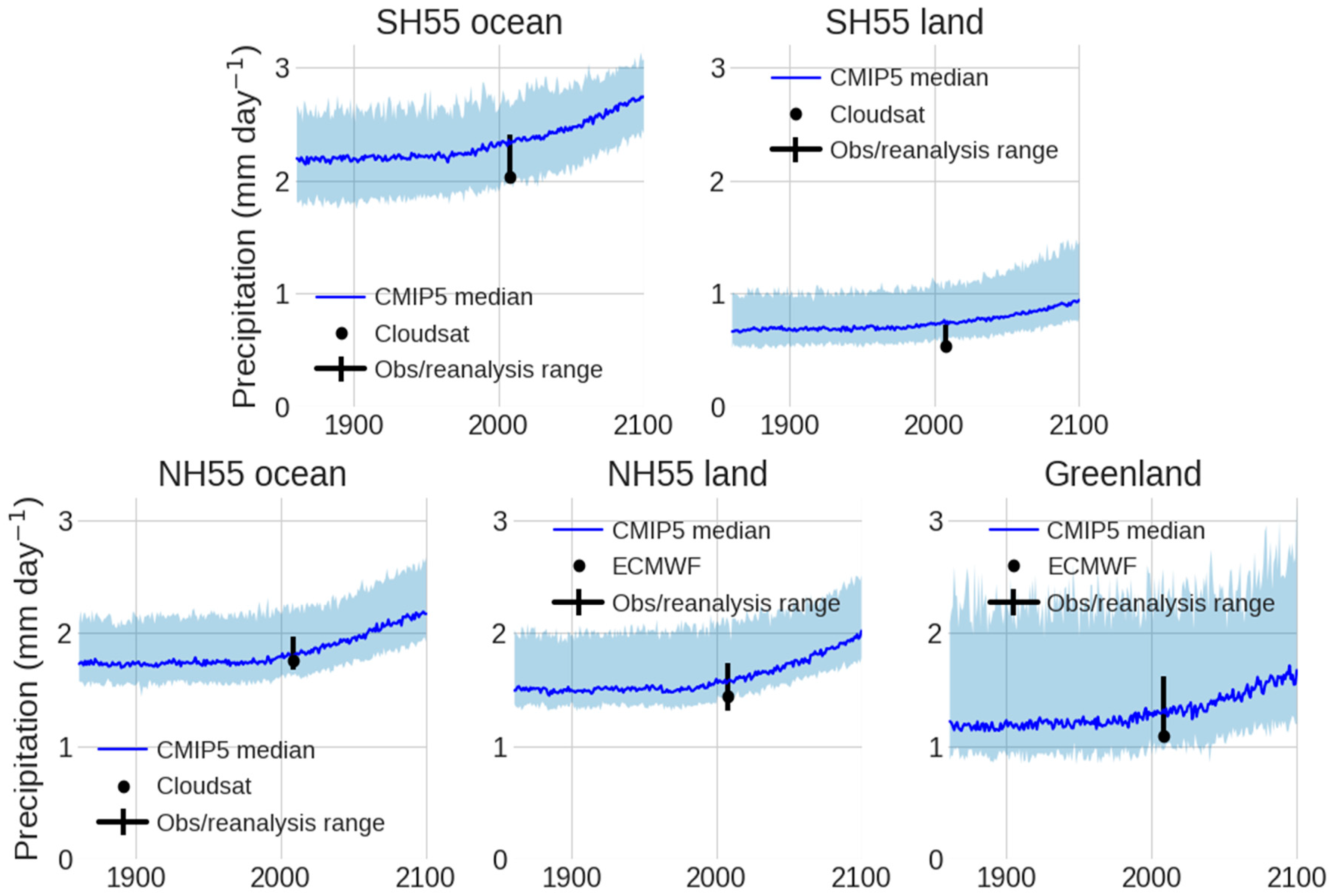
Figure 2 shows the time series of total regional precipitation with the CMIP5 5–95% ensemble range in blue and median as bold blue line for years 1850–2100. Observations and reanalyses (GPCP, CloudSat, MERRA, NCEP, ERA-I) values for 2007–2010 (and based on [12]) are shown as the vertical line with the reference observational product (CloudSat over oceans and Antarctica, and ERA-I over NH land) as a black circle. While in NH the models’ median fall in the range determined by observations and reanalyses, in SH the models’ median exceed this range. Specifically, CloudSat’s Antarctic precipitation estimate is below the 5th percentile of CMIP5, as reported in Palerme et al. [24]. While Behrangi et al. [12] showed agreement between CloudSat and GPCP over Antarctica, CloudSat likely underestimates total snowfall, particularly in the Antarctic interior due to ground clutter and missing shallow precipitation [31].
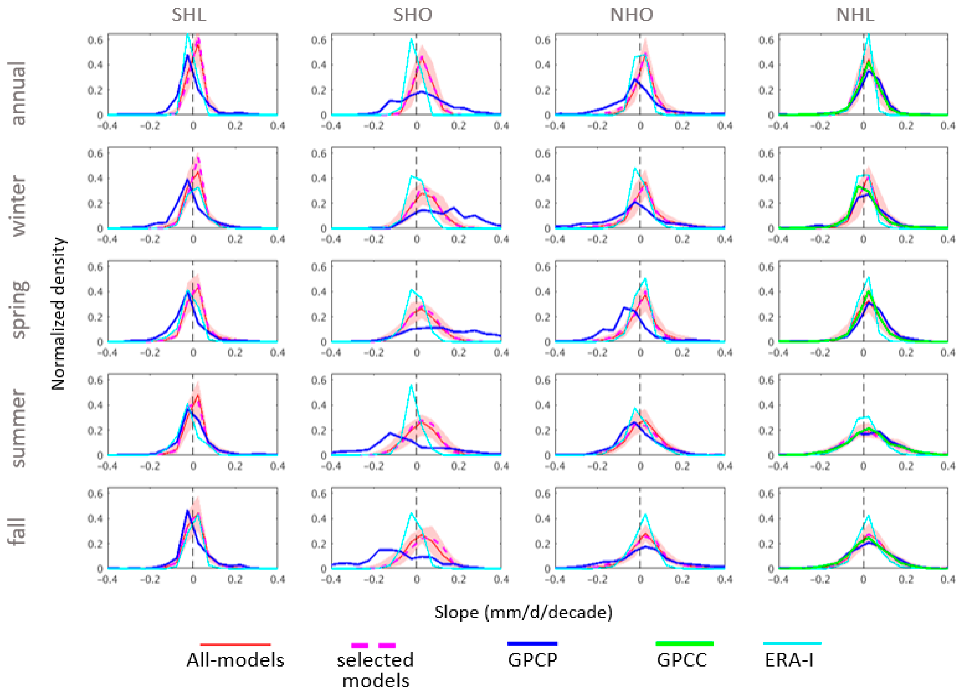
Figure 3 compares normalized density plots of linear trends in precipitation for models, GPCP, ERA-I, and GPCC. The model ensemble 5–95% range is shown in pink and the median as a red line for 1976–2005. GPCP and GPCC plots are constructed from 1980 to 2009 and are shown in blue and green lines, respectively. GPCC is only available for NH land. The dashed magenta lines show the same properties for the five selected models listed in Table 1. The highest model-observation agreement occurs over NH land, where observation products benefit from the availability of ground stations. The trends are least consistent over SH ocean, where GPCP often shows larger positive slopes in winter and spring, and larger negative slopes in summer and fall. ERA-I trends are generally more consistent with models than GPCP, especially over ocean.
4.2. Future Precipitation Changes
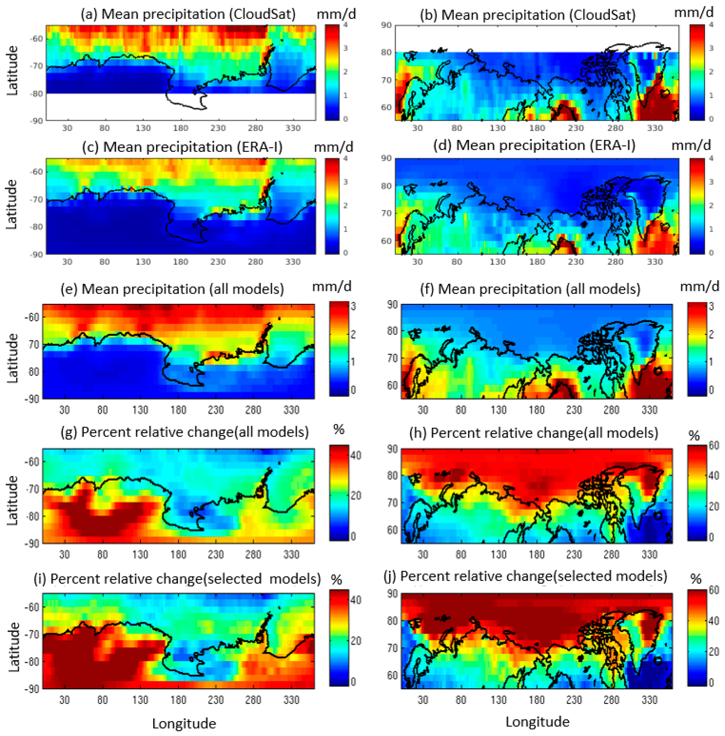
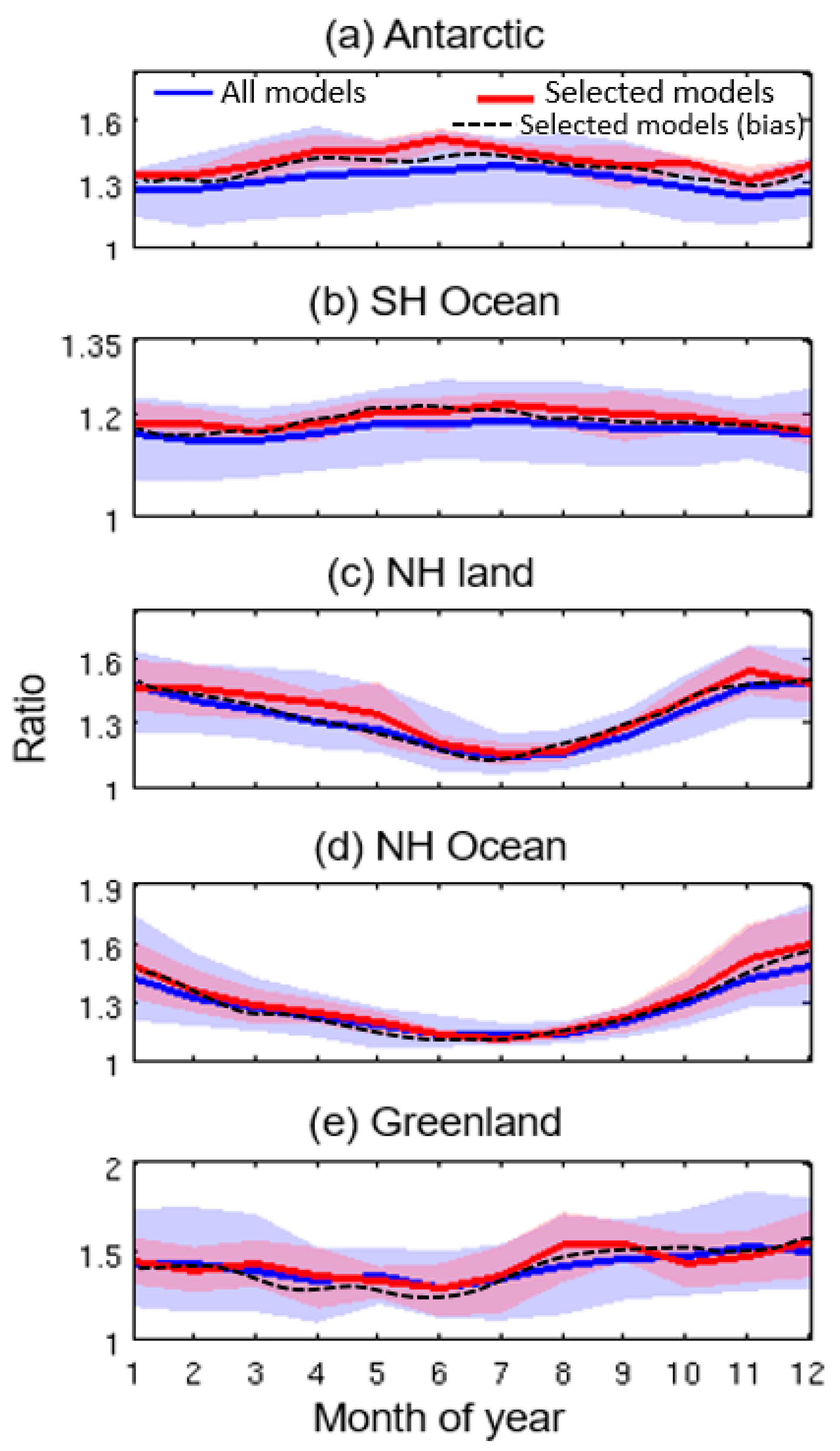
Figure 4 shows maps of annual mean precipitation for 2007–2010 from CloudSat (Figure 4a,b) and ERA-I (Figure 4c,d). It also shows maps of all-model annual mean precipitation for 1976–2005 (Figure 4e,f) and percent precipitation change (by comparing 1971–2100 with 1976–2005) for all (Figure 4g,h) and the selected subset (Figure 4i,j) of models in NH and SH. Figure 4 suggests that while the overall mean precipitation pattern is comparable among the studies products, ERA-I clearly shows lower mean precipitation rate than other products over the Southern Oceans. It can be clearly seen that the selected models suggest a generally larger percentage increase in precipitation than full ensemble average, especially over the Arctic Ocean and Eastern Antarctic ice sheet. The readers are referred to our earlier publication [12] for more detailed comparison between CloudSat precipitation maps and other satellite and reanalysis products. In Figure 5, the fractional regional precipitation changes are plotted separately for each calendar month. The median and 20–80% ensemble range are shown in blue (for all models) and red (for the subset). Also displayed is the median of the same value for the 5 models selected based on bias alone. Figure 5 suggests that modelled colder months experience larger fractional precipitation increases than warmer months, and that the NH regions see greater increases than those in the SH. The selected models generally report larger fractional increase than the full ensemble, with a larger response than that seen when selecting only based on bias. This is more distinct over the Antarctic and SH ocean where the range is above the full ensemble median across almost all months. Meanwhile, this difference is minimal over Greenland compared to the other regions.
The observed larger rate of precipitation increase over land in cold months is consistent with long-term analysis of station data in NH (e.g., [40]) and with the argument that Clausius–Clapeyron relationship determines the increase of large-scale precipitation in winter, while the availability of moisture is the dominant limiting factor in summer [41,42]. However, the largest fractional increase in precipitation also occurs in the cooler months over oceans where moisture supply is not a strong constraint. This implies stronger warming during winter, such as that occurred in past reanalysis for oceans over 20–90°N [43]. Stronger winter warming, relative to summer warming, is also found across the CMIP5 ensemble for high northern latitudes [2]. This is why a common method for assessing precipitation changes is to consider the percentage change per degree of warming [44], and to distinguish between thermodynamic and dynamic contributions to this change [45].
Our combined RMSE + bias method selects a subset that generally shows more warming and faster winter precipitation increase than that based on bias alone. From this we can conclude that those models which better represent the current spatial pattern of precipitation result in greater future warming. The field of emergent constraints, in which observable properties of the current climate state are used to infer future changes, may provide insights on this in future. However, we do not speculate here on why because recent research has shown that identifying robust constraints requires intensive investigation and physical backing [46].
4.3. Mean Precipitation vs. Surface Temperature Change
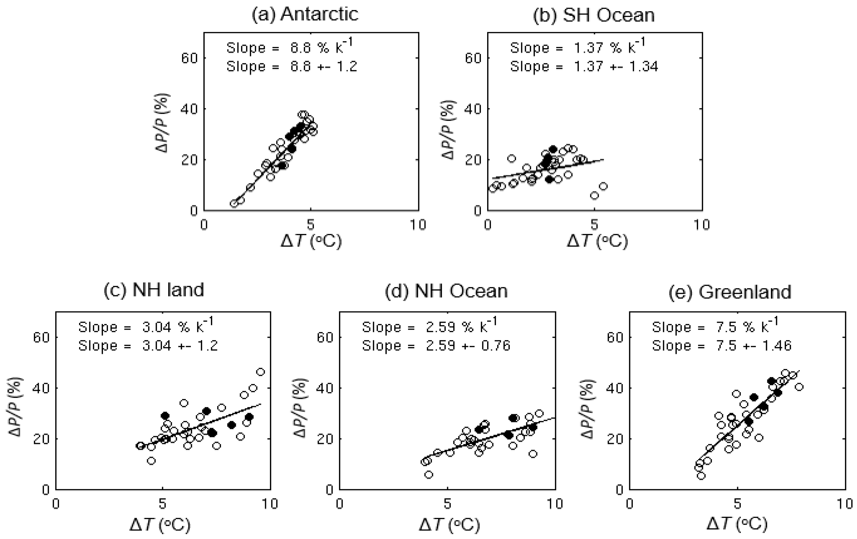
The hydrological sensitivity can be defined by the increase in global mean precipitation for a given change in global mean temperature, and this value can be constrained by the global atmospheric energy budget [23]. The local response of this (ΔP/P)/T can also be estimated, but is not subject to such constraints due to moisture divergence at the boundaries of the region. However, Figure 6 shows that there tend to be consistent responses across the CMIP5 ensemble for each region. In each case, the subset of selected models is shown by filled circles with the others as empty circles. The full ensemble fits are shown for each region, and for the Antarctic, SH ocean, NH land, NH Ocean, and Greenland are 8.8 ± 1.20, 1.37 ± 1.34, 3.04 ± 1.20, 2.59 ± 0.76, and 7.5 ± 1.46%/°C, respectively. Except for the SH ocean, these are larger than the projected global increase of 2%/°C [47]. This is possible due to moisture transport from other regions and the greater net cooling capacity of the atmosphere at these latitudes relative to the global mean. For example, these high latitudes do not experience super greenhouse effects [48,49] that prevent cooling to space as the local surface warms.
The largest calculated slope of 8.8 ± 1.20%/°C is over the Antarctic which is higher than the 3–7.4%/°C that has been reported for regional and global climate models (e.g., [24,50]). From the statistics in Table 2, the strongest correlation between ΔP/P and ΔT occurs in the Antarctic (full ensemble r = 0.93) and the weakest in the SH Ocean (full ensemble r = 0.34). This implies a major role for the Clausius–Clapeyron limit on moisture carrying capacity over Antarctica, but limitations based on either moisture availability or changes in horizontal moisture transport through the region boundaries for the SH oceans. The moisture-availability argument would only apply over sea-ice covered regions.
It can also be seen that the subset of the models generally show larger surface temperature and fractional precipitation change than that full ensemble average, indicating that the larger precipitation changes shown in Figure 6 are largely a result of local thermodynamic effects.
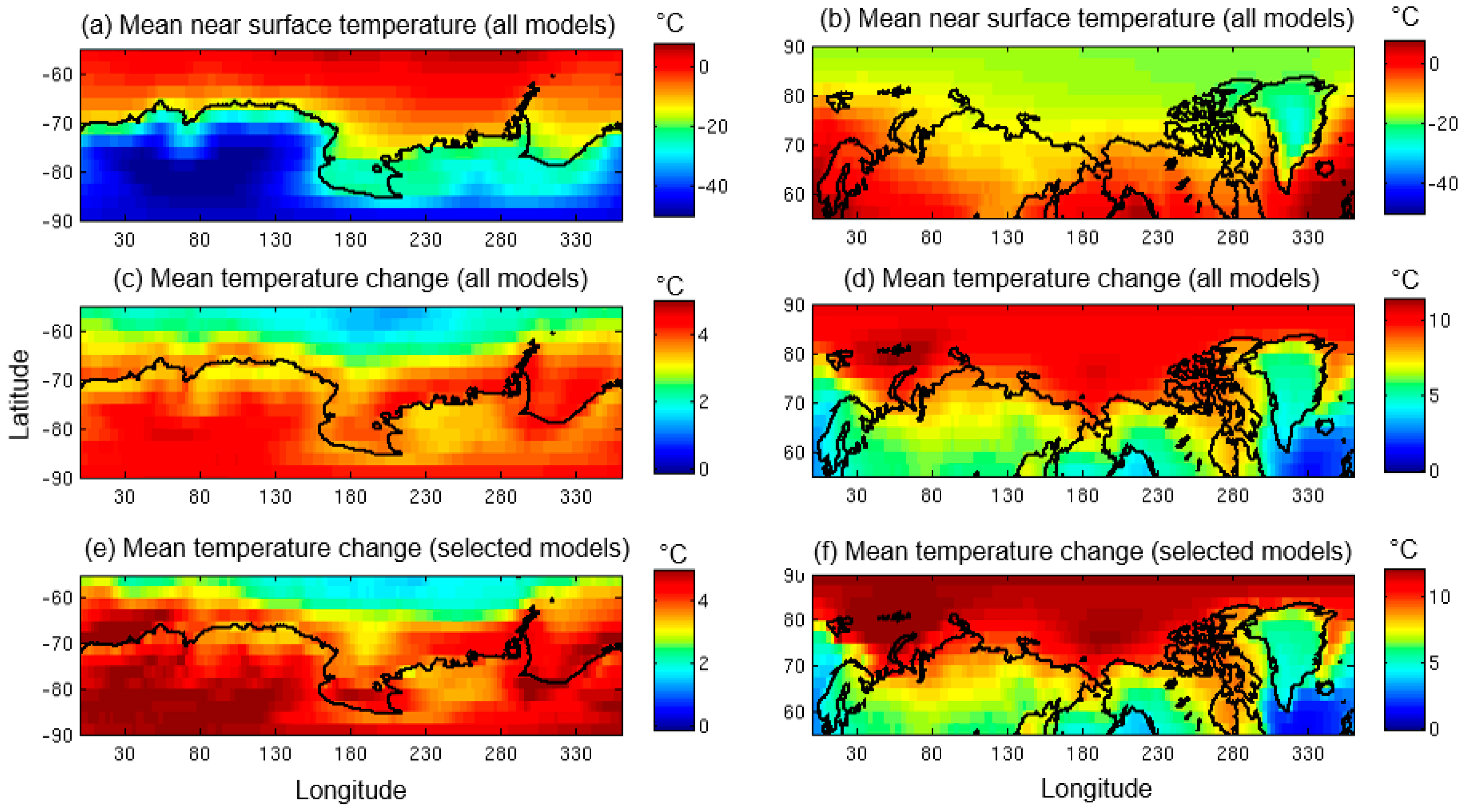
Figure 7 shows maps of mean near surface temperature for 1976–2005 in SH and NH (Figure 7a,b) and its change through 2071–2100 (Figure 7c,d) for the full ensemble mean. The changes are similar to those shown in Figure 4 for relative precipitation change. While temperature tends to increase almost everywhere, the rate of change has strong regional dependence. The selected subset (Figure 7e,f) has a similar spatial pattern but often with larger warming, especially over the Arctic Ocean and East Antarctic ice sheet where the greatest fractional changes in precipitation occurred. The NH generally experiences more warming, especially over the historically ice-covered ocean where the increase in mean surface temperature exceeds 10 °C (Figure 7d) in the full ensemble mean or 12 °C (Figure 7f) in the selected model mean.
4.4. Changes in Spatial Variability
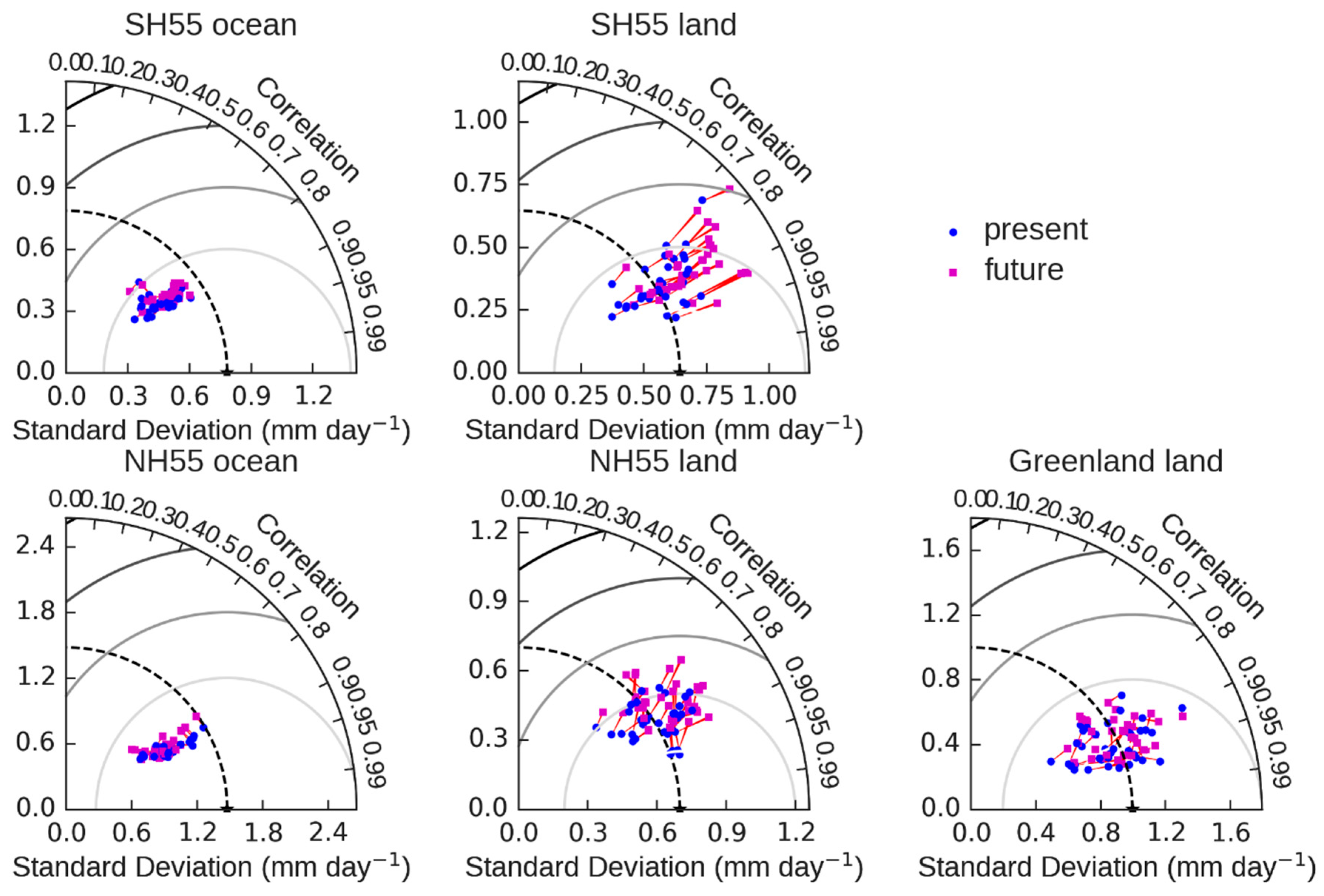
Figure 8 displays Taylor diagrams with present day in blue linked to future values in magenta by red lines. Arcs of constant RMSE are also displayed, with greater distance from the starred reference dataset indicating greater RMSE. Relative to the bottom left corner, any change that extends the radius represents an increase in the spatial variability of precipitation, and any rotation indicates a change in the spatial pattern. Clockwise means that the future simulated pattern is closer to the present day observed pattern, and counterclockwise the opposite.
Inspection of this figure results in the following interpretations:
- (1)
- Over high latitude oceans, only one model shows present or future spatial variability that is as great as that reported by CloudSat, and that one only over the NH55 ocean region.
- (2)
- The greatest inter-model difference in spatial pattern occurs over high latitude land, since they do not fall on a straight radial line,
- (3)
- Both hemispheres’ high latitude land show a general increase in spatial variability. The SH55 land (mainly Antarctica) changes extend radially, indicating little change in the spatial pattern, whereas NH55 land generally show a counterclockwise shift and therefore reduced spatial correlation between present and future.
Point (1) suggests limitations in the simulation of ocean regions of intense precipitation, both in the current and future. Point (2) indicates that the shape and location of the spatial patterns is informative over land. Finally, point (3), with the increased radial extent from present-to-future indicates that these regions generally experience “wet get wetter”, although the angular shift over NH55 land indicates that the location of the wettest and driest regions shifts.
In physical terms, Antarctic precipitation growth mostly occurs on the coast, particularly around the Peninsula and West Antarctic. This occurs in models and in paleoclimate records from historical warmings [50]. The interior is so cold and has such a small current precipitation rate that the faster percentage increase is overwhelmed in terms of mm day−1. The increased spatial standard deviation means that the spread between the wettest and driest regions increases, and with all grid cells in Figure 4 showing increased precipitation this must mean that the wettest areas are getting wetter at a faster rate in absolute terms.
This occurs to some extent over NH land and ocean, but the counterclockwise shift in their future points indicates changes to the pattern of precipitation. This can be inferred from inspection of Figure 4: firstly, the NH ocean south of Greenland shows heavy present day precipitation, but near-zero future changes, for which a number of causes have been proposed [53]. Meanwhile the Bering Sea shows moderate present day precipitation and a substantial future percentage increase. This represents a change in pattern with a decrease in the weighting given to the Atlantic sector. Similar features can be seen over NH land in Figure 4, with major contributions to the correlation between present and future occurring wherever regions of heavy precipitation show small increases, or regions of moderate precipitation show moderate to large fractional increases. Large fractional increases over very dry regions tend to be insufficient to greatly change the spatial correlation. Increases over Finland and the grid cells north of coastal Alaska therefore likely contribute to this change. Further inspection of Figure 4 shows no obvious differences in the spatial patterns, and similar is true for the low-RMSE models in Figure 8. Their future correlation coefficients are not distinguishably different from those of the non-selected models, suggesting that they show similar future patterns of precipitation but with greater mean increase.
5. Summary and Concluding Remarks
Behrangi et al. [12] provided a quantitative observation-based update of precipitation amount and distribution poleward of 55° in the Northern and Southern hemispheres (NH55 and SH55) using various data sets including CloudSat over the oceans and Antarctica to take advantage of its high sensitivity W-band radar. Here, this dataset was used to study simulated high-latitude precipitation and assess future changes in precipitation under the RCP8.5 scenario of large global warming. For NH55 land areas, CloudSat’s products are inappropriate since rain is frequent there and the rain retrieval relies on path-integrated attenuation, which is currently only determined accurately over ocean surfaces. This forced the use of ECMWF Era Interim reanalysis output over NH55 land, although CloudSat was used over Antarctica since its snowfall product does not use path-integrated attenuation.
We selected a subset of models that we identified as better performing based on the smallest discrepancy relative to CloudSat and ERA-I in terms of both the total amount and spatial distribution of high-latitude precipitation. Models within the five lowest sum of rankings for bias + RMSE relative to the reference for a given region are used in our primary analysis.
The use of minimized RMSE is particularly useful as the CloudSat record is only four years, and internal variability can lead to substantial variation between periods of just four years length, meaning that it can only provide a relatively loose constraint. However, CMIP5 models show greater variation in their calculated regional RMSE than they do in total precipitation. The longer GPCP record was split into non-overlapping 4-year periods to estimate the effect of internal variability on this property, and this was found to be smaller than the typical inter-model differences. This finding suggests that the spatial RMSE allows greater discrimination of models based on the limited time series of available data bias. Meanwhile, we continue to use the additional bias criterion to ensure that the total precipitation is also within a realistic range.
We then consider changes in mean precipitation from 1976–2005 to 2071–2100 for the full CMIP5 ensemble and for a subset of 5 selected based on our bias + RMSE rankings. Any such sub-selection of models can be arbitrary, so we clarify that our sub selection of 5 is illustrative only, and the key result is the extra discriminatory power of using spatial RMSE. When selecting models based on bias alone, the detected changes in precipitation under warming are somewhat smaller than when also considering the spatial pattern. This suggests that analysis including spatial patterns may result in somewhat different constraints than are provided by bias alone.
We showed that while colder months experience larger fractional modelled precipitation increases than warmer months, the selected models generally report larger fractional increase than the full ensemble. For everywhere except the SH ocean, the selected models show greater warming than the model ensemble and tend to fall close to the ensemble local hydrological sensitivity trend, indicating that local thermodynamic effects explain much of the change. For the SH ocean, the models that perform best show temperature changes close to the median but precipitation changes greater than those expected from the full ensemble hydrological relationship, implying that a process other than local thermodynamic changes is the main cause. Based on previous findings [24], this may be related to the sea ice coverage and its change, through the way in which sea ice modifies moisture availability.
A Taylor diagram analysis suggests that across the full CMIP5 ensemble, the NH and SH land areas show increased standard deviation of their spatial precipitation patterns, suggesting a “wet get wetter” paradigm for land poleward of 55°. The SH55 land areas show stable correlations, indicative of small changes in the spatial pattern, but this is not true of NH55 land. This is typical of cases where the spatial pattern of precipitation changes through time as well as the differences in precipitation between wet and dry regions.
Here we presented some potentials and challenges for using CloudSat precipitation estimates to assess the climate models in high latitudes. We note that while CloudSat is more capable than other existing spaceborne sensors in detecting the common type of precipitation in high latitudes (i.e., light rain, drizzle, and snowfall), it may also face various uncertainties, among which is an uncertainty in separating precipition phase. This is partly due to lack of dual-frequency radar as well as the temperature-based approach that utilizes reanalysis data. While future instruments may reduce such uncertainty sources, the use of wet-bulb temperature [54,55] instead of air temperature might be helpful in the short term. Furthermore, the short period of CloudSat data limits our comprehensive assessment, the near future launch and operation of the Earth, Clouds, Aerosols, and Radiation Explorer mission (EarthCARE) [56] will provide capabilities comparable to CloudSat that helps produce longer data record and enhance our climate model assessment.
Author Contributions
A.B. and M.R. conceived and designed the experiments; A.B. and M.R. analyzed the data and performed the experiment; A.B. and M.R. wrote the paper.
Funding
This research received no external funding.
Acknowledgments
The research described in this paper was carried out at the University of Arizona and Jet Propulsion Laboratory, California Institute of Technology, under a contract with the National Aeronautics and Space Administration. Financial support was also made available from NASA Energy and Water Cycle Study (NNH13ZDA001N-NEWS), and NASA MEaSUREs (NNH17ZDA001N-MEASURES) awards.
Conflicts of Interest
The authors declare no conflict of interest.
References
- Alexeev, V.A.; Langen, P.L.; Bates, J.R. Polar amplification of surface warming on an aquaplanet in “ghost forcing” experiments without sea ice feedbacks. Clim. Dyn. 2005, 24, 655–666. [Google Scholar] [CrossRef]
- Pithan, F.; Mauritsen, T. Arctic amplification dominated by temperature feedbacks in contemporary climate models. Nat. Geosci. 2014, 7, 181–184. [Google Scholar] [CrossRef]
- Min, S.K.; Zhang, X.; Zwiers, F.W.; Agnew, T. Human influence on arctic sea ice detectable from early 1990s onwards. Geophys. Res. Lett. 2008, 35. [Google Scholar] [CrossRef]
- Vaughan, D.G.; Comiso, J.C.; Allison, I.; Carrasco, J.; Kaser, G.; Kwok, R.; Mote, P.; Murray, T.; Paul, F.; Ren, J.; et al. Observations: Cryosphere. In Climate Change 2013: The Physical Science Basis. Contribution of Working Group I to the Fifth Assessment Report of the Intergovernmental Panel on Climate Change; Stocker, T.F., Ed.; Cambridge University Press: Cambridge, UK; New York, NY, USA, 2013. [Google Scholar]
- Peterson, B.J.; Holmes, R.M.; McClelland, J.W.; Vörösmarty, C.J.; Lammers, R.B.; Shiklomanov, A.I.; Shiklomanov, I.A.; Rahmstorf, S. Increasing river discharge to the arctic ocean. Science 2002, 298, 2171–2173. [Google Scholar] [CrossRef] [PubMed]
- Boening, C.; Lebsock, M.; Landerer, F.; Stephens, G. Snowfall-driven mass change on the east antarctic ice sheet. Geophys. Res. Lett. 2012, 39. [Google Scholar] [CrossRef]
- Zwally, H.J.; Li, J.; Robbins, J.W.; Saba, J.L.; Yi, D.; Brenner, A.C. Mass gains of the antarctic ice sheet exceed losses. J. Glaciol. 2017, 61, 1019–1036. [Google Scholar] [CrossRef]
- Stephens, G.L.; L’Ecuyer, T.; Forbes, R.; Gettelmen, A.; Golaz, J.-C.; Bodas-Salcedo, A.; Suzuki, K.; Gabriel, P.; Haynes, J. Dreary state of precipitation in global models. J. Geophys. Res. Atmos. 2010, 115. [Google Scholar] [CrossRef] [Green Version]
- Adler, R.F.; Gu, G.; Huffman, G.J. Estimating climatological bias errors for the global precipitation climatology project (gpcp). J. Appl. Meteorol. Climatol. 2012, 51, 84–99. [Google Scholar] [CrossRef]
- Berg, W.; L’Ecuyer, T.; Kummerow, C. Rainfall climate regimes: The relationship of regional trmm rainfall biases to the environment. J. Appl. Meteorol. Climatol. 2006, 45, 434–454. [Google Scholar] [CrossRef]
- Lebsock, M.D.; L’Ecuyer, T.S. The retrieval of warm rain from cloudsat. J. Geophys. Res. Atmos. 2011, 116. [Google Scholar] [CrossRef]
- Behrangi, A.; Christensen, M.; Richardson, M.; Lebsock, M.; Stephens, G.; Huffman, G.J.; Bolvin, D.; Adler, R.F.; Gardner, A.; Lambrigtsen, B.; et al. Status of high-latitude precipitation estimates from observations and reanalyses. J. Geophys. Res. Atmos. 2016, 121, 4468–4486. [Google Scholar] [CrossRef] [PubMed]
- Adler, R.; Sapiano, M.; Huffman, G.; Wang, J.-J.; Gu, G.; Bolvin, D.; Chiu, L.; Schneider, U.; Becker, A.; Nelkin, E.; et al. The global precipitation climatology project (GPCP) monthly analysis (new version 2.3) and a review of 2017 global precipitation. Atmosphere 2018, 9, 138. [Google Scholar] [CrossRef] [PubMed]
- Huffman, G.J.; Adler, R.F.; Bolvin, D.T.; Gu, G. Improving the global precipitation record: GPCP version 2.1. Geophys. Res. Lett. 2009, 36. [Google Scholar] [CrossRef]
- Schneider, U.; Becker, A.; Finger, P.; Meyer-Christoffer, A.; Ziese, M.; Rudolf, B. GPCC’s new land surface precipitation climatology based on quality-controlled in situ data and its role in quantifying the global water cycle. Theor. Appl. Climatol. 2013, 115, 15–40. [Google Scholar] [CrossRef]
- Kanamitsu, M.; Ebisuzaki, W.; Woollen, J.; Yang, S.-K.; Hnilo, J.J.; Fiorino, M.; Potter, G.L. NCEP-DOE AMIP-ii reanalysis (r-2). Bull. Am. Meteorol. Soc. 2002, 83, 1631–1644. [Google Scholar] [CrossRef]
- Dee, D.P.; Uppala, S.M.; Simmons, A.J.; Berrisford, P.; Poli, P.; Kobayashi, S.; Andrae, U.; Balmaseda, M.A.; Balsamo, G.; Bauer, P.; et al. The era-interim reanalysis: Configuration and performance of the data assimilation system. Q. J. R. Meteorol. Soc. 2011, 137, 553–597. [Google Scholar] [CrossRef]
- Rienecker, M.M.; Suarez, M.J.; Gelaro, R.; Todling, R.; Bacmeister, J.; Liu, E.; Bosilovich, M.G.; Schubert, S.D.; Takacs, L.; Kim, G.K.; et al. Merra: NASA’s modern-era retrospective analysis for research and applications. J. Clim. 2011, 24, 3624–3648. [Google Scholar] [CrossRef]
- Bosilovich, M.G.; Robertson, F.R.; Chen, J. Global energy and water budgets in merra. J. Clim. 2011, 24, 5721–5739. [Google Scholar] [CrossRef]
- Kumar, S.; Merwade, V.; Kinter, J.L.; Niyogi, D. Evaluation of temperature and precipitation trends and long-term persistence in CMIP5 twentieth-century climate simulations. J. Clim. 2013, 26, 4168–4185. [Google Scholar] [CrossRef]
- Gu, G.; Adler, R.F.; Huffman, G.J. Long-term changes/trends in surface temperature and precipitation during the satellite era (1979–2012). Clim. Dyn. 2015, 46, 1091–1105. [Google Scholar] [CrossRef]
- Tapiador, F.J.; Behrangi, A.; Haddad, Z.S.; Katsanos, D.; de Castro, M. Disruptions in precipitation cycles: Attribution to anthropogenic forcing. J. Geophys. Res. Atmos. 2016, 121, 2161–2177. [Google Scholar] [CrossRef]
- DeAngelis, A.M.; Qu, X.; Zelinka, M.D.; Hall, A. An observational radiative constraint on hydrologic cycle intensification. Nature 2015, 528, 249–253. [Google Scholar] [CrossRef] [PubMed]
- Palerme, C.; Genthon, C.; Claud, C.; Kay, J.E.; Wood, N.B.; L’Ecuyer, T. Evaluation of current and projected antarctic precipitation in cmip5 models. Clim. Dyn. 2017, 48, 225–239. [Google Scholar] [CrossRef]
- Hirota, N.; Takayabu, Y.N.; Hamada, A. Reproducibility of summer precipitation over northern Eurasia in CMIP5 multiclimate models. J. Clim. 2016, 29, 3317–3337. [Google Scholar] [CrossRef]
- Behrangi, A.; Lebsock, M.; Wong, S.; Lambrigtsen, B. On the quantification of oceanic rainfall using spaceborne sensors. J. Geophys. Res. Atmos. 2012, 117. [Google Scholar] [CrossRef] [Green Version]
- Behrangi, A.; Tian, Y.; Lambrigtsen, B.H.; Stephens, G.L. What does cloudsat reveal about global land precipitation detection by other spaceborne sensors? Water Resour. Res. 2014, 50, 4893–4905. [Google Scholar] [CrossRef]
- Behrangi, A.; Stephens, G.; Adler, R.F.; Huffman, G.J.; Lambrigtsen, B.; Lebsock, M. An update on the oceanic precipitation rate and its zonal distribution in light of advanced observations from space. J. Clim. 2014, 27, 3957–3965. [Google Scholar] [CrossRef]
- Palerme, C.; Kay, J.E.; Genthon, C.; L’Ecuyer, T.; Wood, N.B.; Claud, C. How much snow falls on the antarctic ice sheet? Cryosphere Discuss. 2014, 8, 1279–1304. [Google Scholar] [CrossRef]
- Haynes, J.M.; L’Ecuyer, T.S.; Stephens, G.L.; Miller, S.D.; Mitrescu, C.; Wood, N.B.; Tanelli, S. Rainfall retrieval over the ocean with spaceborne w-band radar. J. Geophys. Res. 2009, 114. [Google Scholar] [CrossRef]
- Wood, N.B.; L’Ecuyer, T.S.; Heymsfield, A.J.; Stephens, G.L.; Hudak, D.R.; Rodriguez, P. Estimating snow microphysical properties using collocated multisensor observations. J. Geophys. Res. Atmos. 2014, 119, 8941–8961. [Google Scholar] [CrossRef] [Green Version]
- Norin, L.; Devasthale, A.; L’Ecuyer, T.S.; Wood, N.B.; Smalley, M. Intercomparison of snowfall estimates derived from the cloudsat cloud profiling radar and the ground-based weather radar network over Sweden. Atmos. Meas. Tech. 2015, 8, 5009–5021. [Google Scholar] [CrossRef]
- Cao, Q.; Hong, Y.; Chen, S.; Gourley, J.J.; Zhang, J.; Kirstetter, P.E. Snowfall detectability of nasa’s cloudsat: The first cross-investigation of its 2c-snow-profile product and national multi-sensor mosaic qpe (nmq) snowfall data. Prog. Electromagn. Res. 2014, 148, 55–61. [Google Scholar] [CrossRef]
- Tanelli, S.; Durden, S.L.; Im, E.; Pak, K.S.; Reinke, D.G.; Partain, P.; Haynes, J.M.; Marchand, R.T. Cloudsat’s cloud profiling radar after two years in orbit: Performance, calibration, and processing. IEEE Trans. Geosci. Remote Sens. 2008, 46, 3560–3573. [Google Scholar] [CrossRef]
- Grazioli, J.; Madeleine, J.B.; Gallee, H.; Forbes, R.M.; Genthon, C.; Krinner, G.; Berne, A. Katabatic winds diminish precipitation contribution to the antarctic ice mass balance. Proc. Natl. Acad. Sci. USA 2017, 114, 10858–10863. [Google Scholar] [CrossRef] [PubMed]
- Medley, B.; Joughin, I.; Das, S.B.; Steig, E.J.; Conway, H.; Gogineni, S.; Criscitiello, A.S.; McConnell, J.R.; Smith, B.E.; Broeke, M.R.; et al. Airborne-radar and ice-core observations of annual snow accumulation over thwaites glacier, west antarctica confirm the spatiotemporal variability of global and regional atmospheric models. Geophys. Res. Lett. 2013, 40, 3649–3654. [Google Scholar] [CrossRef]
- Bromwich, D.H.; Nicolas, J.P.; Monaghan, A.J. An assessment of precipitation changes over antarctica and the Southern Ocean since 1989 in contemporary global reanalyses. J. Clim. 2011, 24, 4189–4209. [Google Scholar] [CrossRef]
- Taylor, K.E.; Stouffer, R.J.; Meehl, G.A. An overview of cmip5 and the experiment design. Bull. Am. Meteorol. Soc. 2012, 93, 485–498. [Google Scholar] [CrossRef]
- Moss, R.H.; Edmonds, J.A.; Hibbard, K.A.; Manning, M.R.; Rose, S.K.; van Vuuren, D.P.; Carter, T.R.; Emori, S.; Kainuma, M.; Kram, T.; et al. The next generation of scenarios for climate change research and assessment. Nature 2010, 463, 747. [Google Scholar] [CrossRef] [PubMed]
- Ye, H.; Fetzer, E.J. Atmospheric moisture content associated with surface air temperatures over northern eurasia. Int. J. Climatol. 2010, 30, 1463–1471. [Google Scholar] [CrossRef]
- Berg, P.; Haerter, J.O.; Thejll, P.; Piani, C.; Hagemann, S.; Christensen, J.H. Seasonal characteristics of the relationship between daily precipitation intensity and surface temperature. J. Geophys. Res. Atmos. 2009, 114. [Google Scholar] [CrossRef] [Green Version]
- Ye, H.; Fetzer, E.J.; Wong, S.; Behrangi, A.; Olsen, E.T.; Cohen, J.; Lambrigtsen, B.H.; Chen, L. Impact of increased water vapor on precipitation efficiency over northern Eurasia. Geophys. Res. Lett. 2014, 41, 2941–2947. [Google Scholar] [CrossRef]
- Cohen, J.L.; Furtado, J.C.; Barlow, M.; Alexeev, V.A.; Cherry, J.E. Asymmetric seasonal temperature trends. Geophys. Res. Lett. 2012, 39. [Google Scholar] [CrossRef] [Green Version]
- Seager, R.; Naik, N.; Vecchi, G.A. Thermodynamic and dynamic mechanisms for large-scale changes in the hydrological cycle in response to global warming. J. Clim. 2010, 23, 4651–4668. [Google Scholar] [CrossRef]
- Kleidon, A.; Kravitz, B.; Renner, M. The hydrological sensitivity to global warming and solar geoengineering derived from thermodynamic constraints. Geophys. Res. Lett. 2015, 42, 138–144. [Google Scholar] [CrossRef] [Green Version]
- Caldwell, P.M.; Zelinka, M.D.; Klein, S.A. Evaluating emergent constraints on equilibrium climate sensitivity. J. Clim. 2018, 31, 3921–3942. [Google Scholar] [CrossRef]
- Held, I.M.; Soden, B.J. Robust responses of the hydrological cycle to global warming. J. Clim. 2006, 19, 5686–5699. [Google Scholar] [CrossRef]
- Valero, F.P.J.; Collins, W.D.; Pilewskie, P.; Bucholtz, A.; Flatau, P.J. Direct radiometric observations of the water vapor greenhouse effect over the equatorial Pacific Ocean. Science 1997, 275, 1773–1776. [Google Scholar] [CrossRef] [PubMed]
- Stephens, G.L.; Kahn, B.H.; Richardson, M. The super greenhouse effect in a changing climate. J. Clim. 2016, 29, 5469–5482. [Google Scholar] [CrossRef]
- Frieler, K.; Clark, P.U.; He, F.; Buizert, C.; Reese, R.; Ligtenberg, S.R.M.; van den Broeke, M.R.; Winkelmann, R.; Levermann, A. Consistent evidence of increasing antarctic accumulation with warming. Nat. Clim. Chang. 2015, 5, 348–352. [Google Scholar] [CrossRef]
- Armour, K.C.; Bitz, C.M.; Roe, G.H. Time-Varying Climate Sensitivity from Regional Feedbacks. J. Clim. 2013, 26, 4518–4534. [Google Scholar] [CrossRef] [Green Version]
- Rugenstein, M.A.; Caldeira, K.; Knutti, R. Dependence of global radiative feedbacks on evolving patterns of surface heat fluxes. Geophys. Res. Lett. 2016, 43, 9877–9885. [Google Scholar] [CrossRef]
- Hand, R.; Keenlyside, N.S.; Omrani, N.-E.; Bader, J.; Greatbatch, R.J. The role of local sea surface temperature pattern changes in shaping climate change in the North Atlantic sector. Clim. Dyn. 2018. [Google Scholar] [CrossRef]
- Sims, E.M.; Liu, G. A parameterization of the probability of snow-rain transition. J. Hydrometeorol. 2015, 16, 1466–1477. [Google Scholar] [CrossRef]
- Behrangi, A.; Yin, X.; Rajagopal, S.; Stampoulis, D.; Ye, H. On distinguishing snowfall from rainfall using near-surface atmospheric information: Comparative analysis, uncertainties, and hydrologic importance. Q. J. R. Meteorol. Soc. 2018. [Google Scholar] [CrossRef]
- Illingworth, A.J.; Barker, H.W.; Beljaars, A.; Ceccaldi, M.; Chepfer, H.; Clerbaux, N.; Cole, J.; Delanoë, J.; Domenech, C.; Donovan, D.P.; et al. The earthcare satellite: The next step forward in global measurements of clouds, aerosols, precipitation, and radiation. Bull. Am. Meteorol. Soc. 2015, 96, 1311–1332. [Google Scholar] [CrossRef]
Figure 1.
(a) mean 4-year average precipitation for each labelled region in GPCP and (b) mean 4-year RMSE compared with the 1990–2015 average in GPCP. The points are plotted at the center of each 4-year period.
Figure 1.
(a) mean 4-year average precipitation for each labelled region in GPCP and (b) mean 4-year RMSE compared with the 1990–2015 average in GPCP. The points are plotted at the center of each 4-year period.

Figure 2.
Time series of total regional precipitation with CMIP5 5–95% ensemble range in blue and median as bold blue line for years 1850–2100. Observations and reanalyses (GPCP, CloudSat, MERRA, NCEP, ERA-I) values for 2007–2010 (and based on Behrangi et al., 2016) are shown as the vertical line with the reference observational product (CloudSat over oceans and Antarctica, and ERA-I over NH land) as a black circle.

Figure 3.
Normalized density plot of precipitation slopes calculated in each grid using 30 years of model (1976–2005), GPCP (1980–2009), GPCC (1980–2009), and ERA-I (1980–2009) data. Models 5–95% ensemble range is shown in pink shades and median as red line. Density plots are shown for four geographical regions. NH land includes land areas north of 55°N and Greenland.

Figure 4.
Maps of annual mean precipitation for 2007–2010 from CloudSat (a,b) and ERA-I (c,d). It also shows maps of all-model annual mean precipitation for 1976–2005 (e,f) and percent precipitation change (by comparing 1971–2100 with 1976–2005) for all-model (g,h) and the selected subset (i,j) of models in NH and SH. The areas near the North and South poles that are not covered by CloudSat maps are shown in white color.

Figure 5.
The ratio of future mean precipitation (2071–2100) over the present climate is plotted separately for each month and each region. The median and 20–80% ensemble range of models are shown using line and shaded areas in blue (for all models) and red (for the subset of selected models) in each region.

Figure 6.
Regional-mean precipitation change (ΔP/P) with respect to surface temperature change (ΔT) for all-models. The subset of selected models in each region is shown by filled-circles, so it can be distinguished from the rest of the models shown by empty circles. The changes are based on comparing the current (1976–2005) and future (1971–2100) climates.

Figure 7.
Similar to Figure 4e–j, but for near surface temperature change (°C).
Figure 7.
Similar to Figure 4e–j, but for near surface temperature change (°C).

Figure 8.
Taylor Diagrams of present and future precipitation for each of the studied high-latitude regions. The reference is shown as a star on the bottom axis in each case, and is CloudSat for SH55 land, SH55 ocean and NH55 ocean. For the others it is ECMWF ERA-I. CMIP5 1976–2005 averages are in blue and 2070–2099 in magenta, with red lines linking each simulation’s change.


Table 1.
The list of the models used in this study. For each study region the selected models based on Bias, RMSE, or both are labeled by “B”, “R”, or “X”, respectively. ANT and GL are for Antarctica and Greenland.
Table 1.
The list of the models used in this study. For each study region the selected models based on Bias, RMSE, or both are labeled by “B”, “R”, or “X”, respectively. ANT and GL are for Antarctica and Greenland.
| Models | ANT | NH Ocean | SH Ocean | NH Land | GL | Models | ANT | NH Ocean | SH Ocean | NH Land | GL |
|---|---|---|---|---|---|---|---|---|---|---|---|
| NorESM1-M | X | GFDL-ESM2M | X | ||||||||
| CMCC-CMS | X | X | bcc-csm1-1-m | ||||||||
| NorESM1-ME | X | X | CNRM-CM5 | ||||||||
| MPI-ESM-MR | MRI-CGCM3 | X | X | ||||||||
| GISS-E2-R | MIROC-ESM | ||||||||||
| MPI-ESM-LR | MIROC-ESM-CHEM | ||||||||||
| GISS-E2-R-CC | MRI-ESM1 | ||||||||||
| GFDL-CM3 | HadGEM2-CC | X | X | X | X | ||||||
| CSIRO-Mk3-6-0 | X | GISS-E2-H | X | ||||||||
| CMCC-CESM | HadGEM2-ES | ||||||||||
| CMCC-CM | ACCESS1-0 | X | |||||||||
| bcc-csm1-1 | X | ACCESS1-3 | X | ||||||||
| CCSM4 | X | X | FGOALS-g2 | ||||||||
| CESM1-CAM5 | X | X | X | inmcm4 | |||||||
| CESM1-BGC | HadGEM2-AO | ||||||||||
| GFDL-ESM2G | MIROC5 | X | X | ||||||||
| CanESM2 | X | FIO-ESM | |||||||||
| GISS-E2-H-CC | BNU-ESM |
Table 2.
Statistics for surface temperature and percent relative precipitation change for all and subset models. The table is constructed using the same data plotted in Figure 6.
Table 2.
Statistics for surface temperature and percent relative precipitation change for all and subset models. The table is constructed using the same data plotted in Figure 6.
| ΔT (°C) | ΔP/P (%) | Correlation | ||||||
|---|---|---|---|---|---|---|---|---|
| Models | min | max | mean | min | max | mean | Coefficient | |
| Antarctic | All | 1.43 | 5.12 | 3.79 | 2.63 | 37.59 | 23.26 | 0.93 |
| subset | 3.68 | 4.53 | 4.12 | 17.46 | 33.12 | 26.95 | 0.89 | |
| SH ocean | All | 0.27 | 5.44 | 2.75 | 5.68 | 24.50 | 15.88 | 0.34 |
| subset | 2.75 | 3.06 | 2.88 | 12.06 | 24.07 | 18.75 | 0.33 | |
| NH land | All | 3.21 | 7.86 | 5.35 | 5.44 | 45.71 | 27.54 | 0.87 |
| subset | 5.56 | 6.92 | 6.22 | 26.52 | 42.68 | 35.12 | 0.76 | |
| NH ocean | All | 3.97 | 9.58 | 6.44 | 11.32 | 46.29 | 23.98 | 0.66 |
| subset | 5.09 | 9.06 | 7.34 | 22.18 | 30.50 | 27.12 | −0.23 | |
| Greenland | All | 3.96 | 10.87 | 7.12 | 5.64 | 32.48 | 20.64 | 0.77 |
| subset | 6.48 | 10.15 | 8.31 | 21.29 | 27.97 | 24.91 | 0.53 | |
© 2018 by the authors. Licensee MDPI, Basel, Switzerland. This article is an open access article distributed under the terms and conditions of the Creative Commons Attribution (CC BY) license (http://creativecommons.org/licenses/by/4.0/).
Share and Cite
MDPI and ACS Style
Behrangi, A.; Richardson, M. Observed High-Latitude Precipitation Amount and Pattern and CMIP5 Model Projections. Remote Sens. 2018, 10, 1583. https://doi.org/10.3390/rs10101583
AMA Style
Behrangi A, Richardson M. Observed High-Latitude Precipitation Amount and Pattern and CMIP5 Model Projections. Remote Sensing. 2018; 10(10):1583. https://doi.org/10.3390/rs10101583
Chicago/Turabian StyleBehrangi, Ali, and Mark Richardson. 2018. "Observed High-Latitude Precipitation Amount and Pattern and CMIP5 Model Projections" Remote Sensing 10, no. 10: 1583. https://doi.org/10.3390/rs10101583
Note that from the first issue of 2016, this journal uses article numbers instead of page numbers. See further details here.