Spatial-Temporal Changes of Soil Organic Carbon Content in Wafangdian, China

Abstract

Soil organic carbon (SOC) plays an important role in soil fertility and the global carbon cycle. A better understanding of spatial-temporal changes of SOC content is essential for soil resource management, emission studies, and carbon accounting. In this study, we used a boosted regression trees (BRT) model to map distributions of SOC content in the topsoil (0–20 cm) and evaluated its temporal dynamics from 1990–2010 in Wafangdian City, northeast of China. A set of 110 (1990) and 127 (2010) soil samples were collected and nine environment variables (including topography and vegetation) were used. A 10-fold cross-validation was used to evaluate model performance as well as predictive uncertainty. Accuracy assessments showed that R² of 0.53 and RMSE (Root-mean-square error) of 9.7 g∙kg⁻¹ for 1990, and 0.55, and 5.2 g∙kg⁻¹ for 2010. Elevation and NDVI (Normalized Difference Vegetation Index) were the two important variables affecting SOC distribution. Results showed that mean SOC content decreased from 19 ± 14 to 18 ± 8 g∙kg⁻¹ over a 20 year period. The maps of SOC represented a decreasing trend from south to north across the study area in both periods. Rapid urbanization and land-use changes were accountable for declining SOC levels. We believe predicted maps of SOC can help local land managers and government agencies to evaluate soil quality and assess carbon sequestration potential and carbon credits.

1. Introduction

Soil organic carbon (SOC) is the largest terrestrial carbon pool and plays an important role in the global carbon cycle [1,2,3,4]. It determines the fate of a terrestrial ecosystem as a potential sink or a source of greenhouse gases [5]. In addition, SOC is closely related to soil quality, nutrient availability and crop yield [5]. Its decomposition can increase atmospheric CO₂ levels [6], and its sequestration can significantly mitigate global climate change [7]. Changes in land use from native vegetation to agriculture are able to cut down on SOC levels [8,9] and increase atmospheric carbon dioxide concentration [10]. Therefore, studies focusing on the impact of land-use change and environmental variables controlling spatial-temporal dynamics of SOC are important. Especially in China, which is experiencing population expansion, assessment of spatial-temporal changes of soil properties (e.g., SOC) is considered urgent to make policies to regulate actual needs and ecological demand [7,11,12,13,14]. Moreover, reliable, robust and cost-efficient methods for estimating SOC content and its temporal changes are quite essential.

Spatial-temporal variability of SOC content can be estimated by using statistical models that quantify the relationship between SOC content and environmental variables. The number of SOC measurements used in predicting is an issue because it depends on many factors such as scales and costs. It is unlikely to collect sufficient soil samples to reflect the spatial-temporal changes of SOC content at the country scale [7]. Digital soil mapping (DSM) can predict soil properties over large areas based on sparse or discrete samples [14]. Most DSM studies are based on Jenny’s equation [15], which characterizes soils as a function of environmental variables (i.e., climate, organisms, relief, parent material and time). This concept has been employed in numerous DSM techniques such as multiple linear regression [16], linear mixed models [17], random forest (RF) model [18,19,20,21], support vector machines [15], artificial neural networks [22,23], kriging [7] and the boosted regression tree (BRT) model [1,24] for SOC predictions. Despite various DSM techniques available, selecting an optimal method to predict soil properties is not always promising [1,25].

Referring to DSM techniques listed above, BRT is a relatively new tree-based model [22,25] and has rarely been used to model spatial-temporal variability of SOC [26,27]. Compared to the single-tree model, BRT is more powerful and efficient [20,26]. These studies show that BRT is a reliable model in predicting soil parameters. The fitted model in BRT is a simple linear combination of many trees that are fitted iteratively and boosted to reweight poorly modeled observations [22,27,28]. Iterative processes improve the predictive performance and ensure robustness [20,21,22]. BRT can deal with various data types, missing values, outliers, irrelevant predictors and interactions between predictors and provide access to evaluate the fitted model [22,27,28]. Owing to these merits, BRT has been widely applied in various scientific fields, including soil science [22,29], remote sensing [30], environmental science [31], ecology [25] and epidemiology [32]. However, BRT has not yet been applied in spatial-temporal modeling of SOC.

The aim of this study was to use BRT to evaluate spatial-temporal changes in topsoil (0–20 cm) organic carbon content in the northeast of China. The specific objectives were: (1) to map SOC content in 1990 and 2010; (2) to quantify environmental controls of SOC content; and (3) to investigate temporal dynamics of SOC content at a 20 year period (1990–2010).

2. Materials and Methods

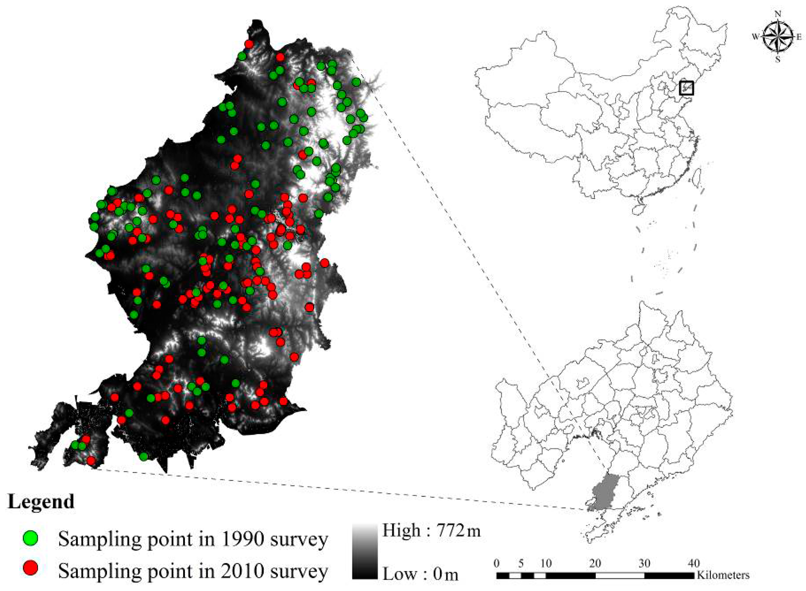
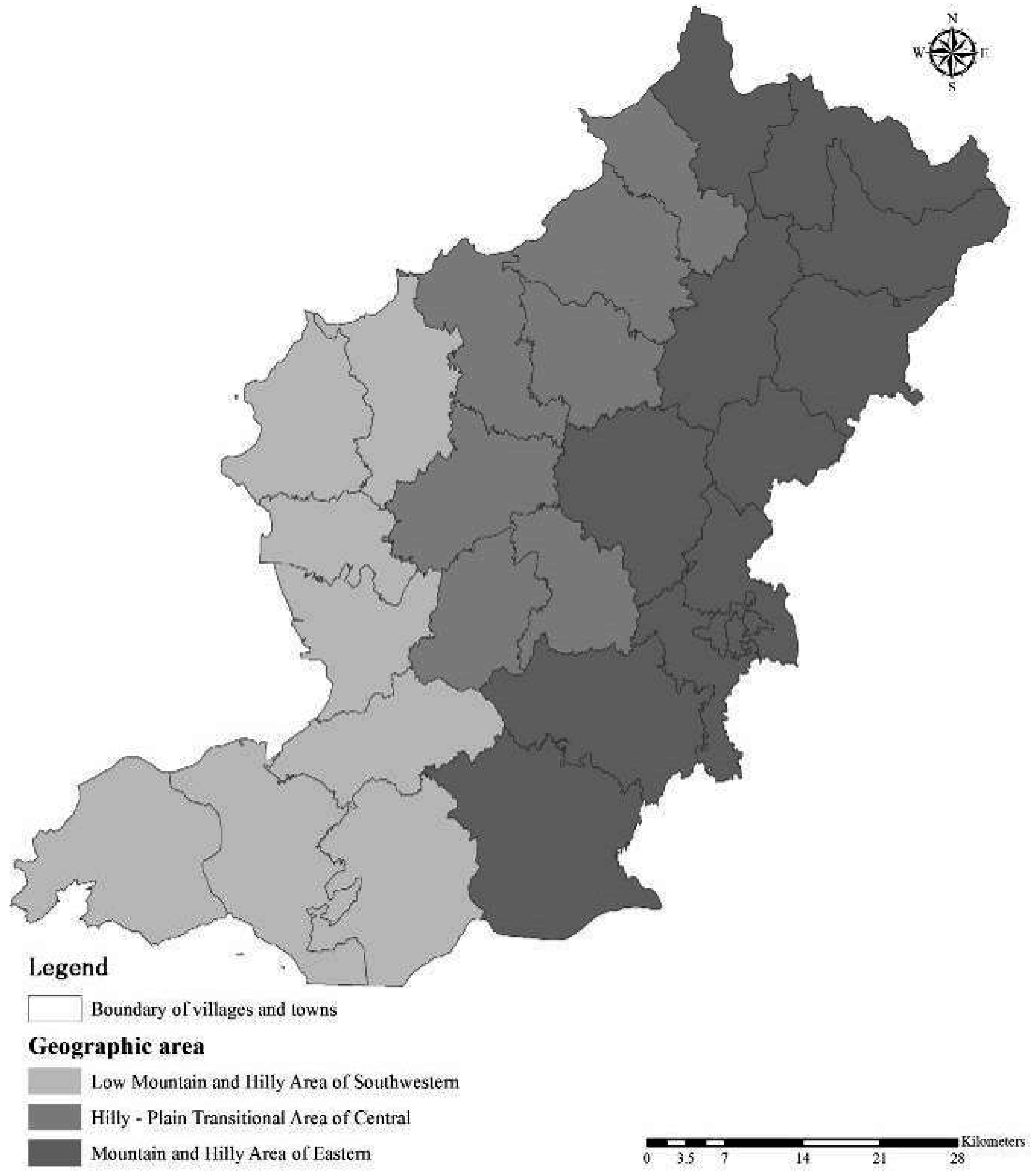
2.1. Study Area

The study was conducted in Wafangdian City, which is located in the southwest of the peninsula of Liaodong in Liaoning province of China (latitude 39°20′–40°07′N; longitude 21°13′–122°16′E) (Figure 1). It covers a total area of 3826.6 km² of which 71% is under agriculture, 13% as garden plots and the rest as construction land used for construction purposes during rapid urbanization. Geomorphologically, the area is characterized by a complex and undulated hill systems intersected by river valleys, which is mostly agriculture dominated. Relative elevation ranges from 0 m to 830 m ASL (Above Sea Level) with an increasing trend from the southwest to the northeast of Wafangdian. The climate is a sub-humid warm temperate continental monsoon type consisting of four seasons, while, in the summer, it is hot and rainy. The mean annual temperature is 9.3 °C, and the mean annual precipitation ranges between 580 to 750 mm. Precipitation of 60%–70% in the study area is concentrated in the summer with frequent rainstorms. Dominant soils in the study area are Cambisols (58%) and Fluvisols (13%) (World Reference Base for Soil Resources (WRB) [33]). Landuse types follow the common land-use system of the northeast of China—agriculture with corn, and soybeans as main crops, and peanuts and fruits in a rotation. Much of the natural vegetation is warm-temperate deciduous broad-leaved forest where the main tree species are Pinaceae, Taxodiaceae, Cupressaceae and Ginkgoaceae. According to the vegetation type and topography, the Wafangdian City is divided into three geographic areas (Low Mountain and Hilly Area of the Southwest vs. the Hilly–Plain Transitional Area of Central vs. Mountain and Hilly Area of Eastern) (Figure 2). With the Chinese economic reform starting in the 1980s, Wafangdian City started to accelerate urbanization and economic development at an unprecedented pace. Due to the dramatic sprawl of rapid urbanization and persistent increase of population, a large number of forests, grasslands, wetlands and others were converted to construction and farmland. Thus, the 1990s was considered the background of this study.

2.2. Collection

2.2.1. Soil Survey Data from 1990

Soil profile data surveyed in 1990 was obtained from the Agro-Technology Extension Center of Wafangdian City. A total of 110 soil profiles were investigated from all land use and soil types (Figure 1). Soil profile data included information on parent material, soil physical and chemical properties, land use and cropping systems. However, the present study focused on SOC content of the topsoil (0–20 cm) only.

2.2.2. Soil Sampling in 2010

Due to rapid land-use change during the past few decades, re-sampling the same sites for a given land-use type from 1990 was not possible. Thus, we designed a purposive sampling to collect a total of 127 topsoil samples representing variations in elevation, aspect, land use and parent material (Figure 1) in 2010, following the methods described in [34]. A handheld global positioning system (GPS) was used to record the geographical location of each sampling site. Soil samples from each location were a composite of five soil cores taken from four corners, and the center of a 1 m × 1 m square area. From the composite sample, 1 kg subsample was retained for laboratory analysis. SOC content of the samples was determined by a wet oxidation method [35] in the Key Laboratory of Agricultural Resources and Environment of Liaoning Province, Shenyang Agricultural University, Shenyang, China.

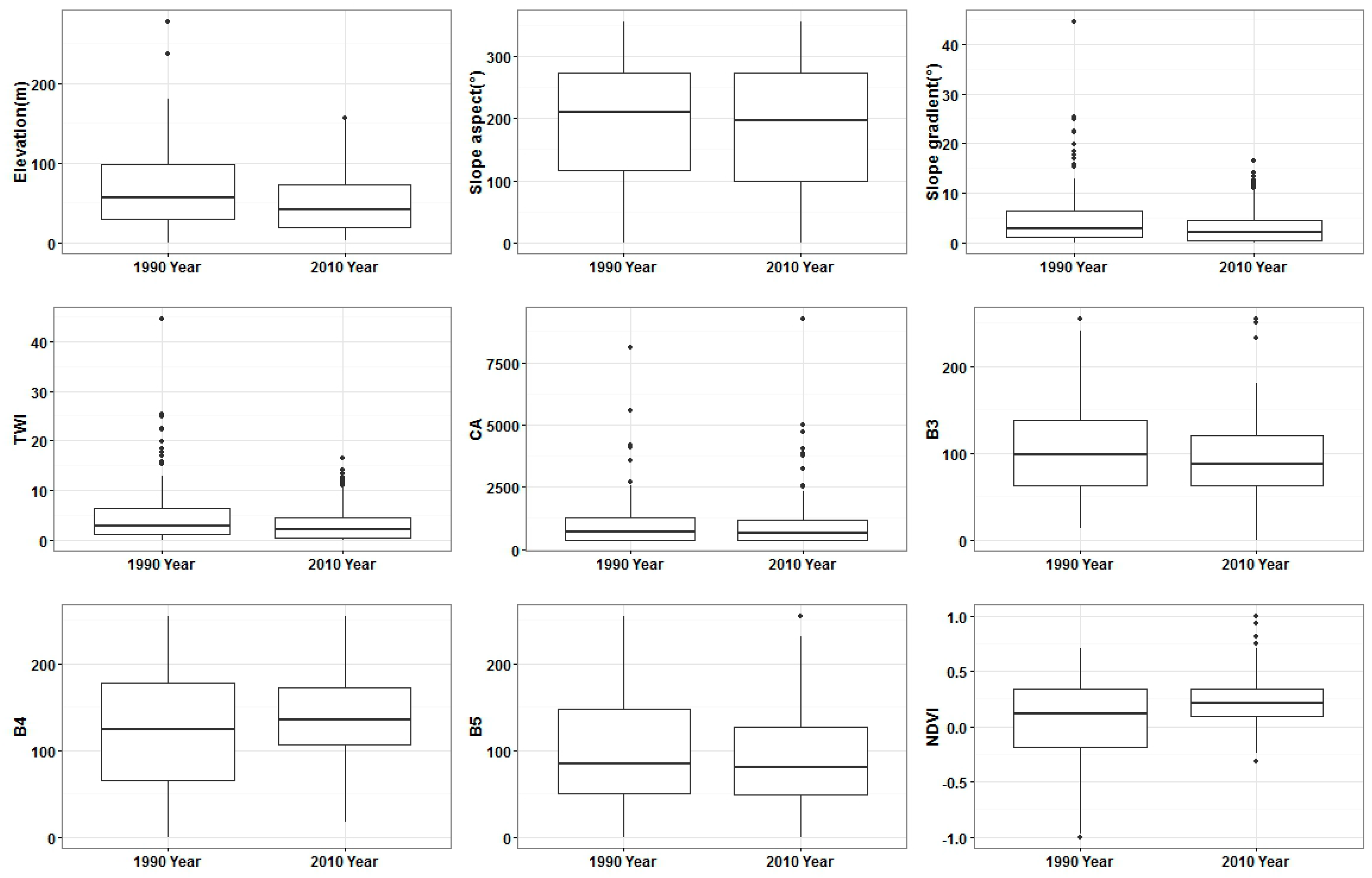
2.2.3. Predictor Variables

Environmental variables used to predict SOC consisted of terrain attributes and remote sensing (RS) data. Terrain attributes were derived from a 90 m × 90 m Digital Elevation Model (DEM) downloaded from the United States Geological Survey (USGS, Reston, VA, USA). It included elevation, slope aspect, slope gradient, topographic wetness index (TWI) and catchment area (CA) calculated in the System for Automated Geoscientific Analyses (SAGA, Hamburg, Germany) GIS [36].

Remote sensing data consisted of six images acquired from July to September (growing season) in 1990 and 2010 with cloud cover less than 10%. The RS data were downloaded from the United States Geological Survey. The images were rectified by polynomial geometric precision correction and mosaicked and trimmed to cover the study area [37]. The data included Landsat Thematic Mapper (Landsat TM) visible red band 3 (B3, 0.63–0.69 μm), near infrared band 4 (B4, 0.78–0.90 μm) and short-wave infrared band 5 (B5, 1.55–1.75 μm). These three bands correspond to vegetation growth, coverage and biomass, respectively [38]. Normalized Difference Vegetation Index (NDVI) was calculated as:

$$\mathrm{NDVI}=\left(\mathrm{band}4-\mathrm{band}3\right)/\left(\mathrm{band}4+\mathrm{band}3\right)$$

(1)

2.2.4. Land-Use Data

Land-use maps were a vector polygon map created from Landsat images from the year 1990 and 2010. Land-use types were grouped into cultivation land, grassland, and forest land, and SOC content in each land use was derived for both periods.

2.3. Prediciton Model Based on Boosted Regression Trees

To quantify the association between environmental variables and SOC, we applied Boosted Regression Trees developed by Friedman et al. [39]. To our knowledge, this study is the first attempt to identify spatial-temporal evolution of SOC using the BRT model. BRT combines two statistical techniques—boosting and regression trees—in a single algorithm. Boosting is based on the stochastic gradient improvement of decision trees by minimizing the loss function (deviation) in the splitting of each tree, and regression trees grow with recursive binary splitting of data until there is some stopping criterion. BRT is flexible to use and yet capable of dealing with complex soil-environmental responses, including interactions and nonlinearities [22,27]. Compared to the traditional regression approach, BRT showed better results in terms of prediction capability [40,41]. BRT performed well in soil properties modeling [42] and has been applied in various studies [27,43]. The BRT script provided by Elith et al. [27] with reference package “dismo” version 0.8-17 [44] and “gbm” version 2.1 [45] were used for model calibration in the R environment [22].

Model fitting in BRT usually required the user to set up four parameters: the learning rate (LR), tree complexity (TC), bag fraction (BF) and number of trees (NT) [22,27,41]. LR represented the contribution of each tree to the final fitted model [22]. TC defined the predictor variables between depth of the tree and the maximum level of interaction [27]. BF represented a proportion of data used in each model—the more data used, the less the randomness [26,28]. Although BRT was a great extension to model over-fitting, it was still necessary to set the optimum number of trees [27]. NT was determined from the combination of LR and TC. For the best predictive performance, various combinations of these parameters were tested to determine optimal settings using 10-fold cross-validation (CV) [27]. We determined the optimum values for these parameters by running many simulations covering a range of LR (0.001–0.05), TC (5–10), BF (0.65–0.85) and NT (500–1000) in the two periods. The final optimal values of LR, TC, BF and NT were set as 0.0025, 9, 600, and 0.70 for the 1990 survey and as 0.0025, 9, 0.65 and 800 for the 2010 survey.

The uncertainty associated with the BRT prediction was evaluated with standard deviation (SD) derived from running the model 100 times and the map was generated as an indicator of SOC prediction uncertainty. To obtain the relative importance (RI) of each predictor, the BRT model was repeated for 100 iterations. The RI of variables were measured based on the number of times a variable was selected for modeling and weighted by the square improvement to each split and averaged across all trees [29]. The RI of each variable was then scaled so that the sum added to 100 as percentages. A higher percentage of a variable indicated a stronger relative importance of this variable on the response [46].

2.4. Model Validation

The performance of the BRT model was evaluated using a 10-fold cross-validation that involved comparisons between predicted and observed SOC values [47]. Cross-validation is a useful approach for model identification and assessment of model performance [22]. Mean absolute prediction error (MAE), root mean square error (RMSE), coefficient of determination (R²) and Lin's concordance correlation coefficient (LCCC) [48] were considered to validate the model and were calculated as follows:

$$\mathrm{MAE}=\frac{1}{n}{\displaystyle \sum _{i=1}^n\left|a_i-b_i\right|}$$

(2)

$$\mathrm{RMSE}=\sqrt{\frac{1}{n}{\displaystyle \sum _{i=1}^n{\left(a_i-b_i\right)}^2}}$$

(3)

$$R^2=\frac{{\displaystyle \sum _{i=1}^n{\left(a_i-{\overline{b}}_i\right)}^2}}{{\displaystyle \sum _{i=1}^n{\left(b_i-{\overline{b}}_i\right)}^2}}$$

(4)

$$\mathrm{LUCC}=\frac{2r{\partial }_a{\partial }_b}{{\partial }_a^2+{\partial }_b^2+{\left(\overline{a}+\overline{b}\right)}^2}$$

(5)

where $a_i$ and $b_i$ are the predicted and observed SOC values at site $i$, respectively; $\overline{a}$ and $\overline{b}$ are the average values of the predicted and observed SOC values; $n$ is the number of samples; ${\partial }_a$ and ${\partial }_b$ are the variances of predicted and observed values; and $r$ is the Pearson correlation coefficient between the observed and predicted values.

3. Results and Discussion

3.1. Descriptive Statistics of SOC Content

The statistical results of SOC content related to land-use types in 1990 and 2010 are shown in

Table 1. Summary statistics of SOC (g∙kg⁻¹) under different land-use patterns in two periods.

Years	Land-Use Pattern	Min	Median	Mean	Max	SD	CV (%)
1990	Cultivated	1.43	7.78	12.45	46.78	11.35	91.12
	Grassland	0.95	17.32	19.30	62.11	14.54	75.32
	Forest	1.65	17.60	21.74	62.11	14.55	66.92
2010	Cultivated	2.38	10.99	10.00	18.76	4.22	42.25
	Grassland	7.18	18.68	19.27	33.98	7.18	37.27
	Forest	12.62	22.49	22.13	32.35	5.54	25.04

Note: SOC, soil organic carbon; SD, standard deviation; CV, coefficient of variation.

. SOC content of cultivated land in 1990 ranged from 1.4 to 46.8 g∙kg⁻¹, with a mean of 12.4 g∙kg⁻¹. Average SOC content of cultivated land in 2010 was 10.0 g∙kg⁻¹ (±4.2 g∙kg⁻¹). Compared to SOC content of cultivated land in 1990, it showed a decreasing trend in 2010, with a narrow range of values. In cultivated land, coefficient of variations (CVs) in 1990 and 2010 were 91.1% and 42.2%, respectively, and SD values were 11.3 and 4.2 g∙kg⁻¹. In grassland and forest, SOC content showed slight changes in both periods. SOC content in all land-use types followed a lognormal distribution and was nearly symmetrically distributed around the mean SOC value in both periods. The relationship between SOC content and environmental variables in 1990 and 2010 is shown in Figure 3.

SOC content varied significantly among geographic areas (Figure 2,

Table 2. SOC content in different geographic areas in 1990 and 2010 surveys.

Geographic Area	1990 SOC (g∙kg−1)			2010 SOC (g∙kg−1)		SOC Change (g∙kg−1)
	Count	Range	Mean ± SD	Count	Range	Mean ± SD
Low Mountain and Hilly Area of the Southwest	37	3.05–62.11	16.56 ± 14.87	37	8.04–33.25	16.08 ± 6.91	−0.48
Hilly–Plain Transitional Area of Central	25	2.35–36.02	16.59 ± 8.78	36	2.38–33.98	12.8 ± 6.69	−3.79
Mountain and Hilly Area of Eastern	48	0.95–61.99	25.15 ± 15.15	54	10.24–33.8	22.31 ± 6.14	−2.84

Note: SD, standard deviation.

), with a decreasing trend from north to south. Hilly–Plain Transitional Area of the Central had the highest decrease of about 4 g∙kg⁻¹. Areas in the Low Mountain and Hilly Area of the Southwest showed a slight decrease (−0.48 g∙kg⁻¹). In the eastern mountain area, forests were converted to plantation crops such as apples, cherries and peaches, in which SOC content decreased by 2.8 g∙kg⁻¹.

Linear correlations between SOC and predictors are shown in

Table 3. Relationships between observed SOC (g∙kg⁻¹) with all predictors in 1990 and 2010 surveys.

Property	SOC	Elevation	Slope Aspect	Slope Gradient	TWI	CA	B3	B4	B5
1990
Elevation	0.37 **
Slope aspect	0.07	0.10
Slope gradient	0.22 *	0.63 **	0.13
TWI	−0.24 *	−0.61 **	−0.44 **	−0.72 **
CA	0.14	0.16	0.11	0.15	−0.34 **
B3	−0.30 **	−0.31 **	0.03	−0.35 **	0.31**	−0.15
B4	0.30 **	0.07	0.05	−0.18	0.06	−0.02	0.32 **
B5	−0.28 **	−0.20 *	0.03	−0.21 *	0.12	−0.02	0.77 **	0.19 *
NDVI	0.53 **	0.42 **	−0.01	0.17	−0.25 **	0.12	−0.38 **	0.62 **	−0.24 *
2010
Elevation	0.73 **
Slope aspect	−0.03	0.00
Slope gradient	0.48 **	0.59 **	0.24 **
TWI	0.24 **	0.22 *	0.25 **	0.36 **
CA	−0.53 **	−0.57 **	−0.22 *	−0.77 **	−0.37 **
B3	−0.08	−0.08	0.04	0.14	0.14	−0.15
B4	−0.07	−0.03	−0.05	0.10	0.11	−0.11	0.60 **
B5	0.05	−0.05	0.01	0.16	0.12	−0.22 *	0.59 **	0.05
NDVI	−0.12	−0.04	−0.06	−0.10	−0.13	0.11	−0.62 **	−0.02	−0.51 **

Note: Significant relationship between two variables with p < 0.05 shown in “*”; Significant relationship between two variables with p < 0.01 shown in “**”. Correlation coefficients (r) and their significance (p) are also presented. CA, catchment area; TWI, topographic wetness index; B3, Landsat TM band 3; B4, Landsat TM band 4; B5, Landsat TM band 5; NDVI, Normalized Difference Vegetation Index.

. SOC was positively correlated with elevation. The coefficient was higher in 2010 (r = 0.73) than in 1990 (r = 0.37). Slope aspect, CA and TWI had higher coefficients with SOC (0.48, −0.53 and 0.24) in 2010 compared to those in 1990. Correlations between SOC and imagery indices were significant in 1990.

3.2. Model Performance

Table 4. Summary statistics of the predictive quality of boosted regression trees (BRT) in 1990 and 2010 for SOC prediction with 100 runs.

Year	Index	Min	Median	Mean	Max	SD
1990	MAE	6.60	6.75	6.75	7.05	0.14
	RMSE	9.46	9.69	9.74	10.24	0.24
	R2	0.43	0.54	0.53	0.61	0.06
	LCCC	0.65	0.70	0.70	0.72	0.03
2010	MAE	4.01	4.05	4.07	4.19	0.07
	RMSE	5.14	5.22	5.26	5.42	0.09
	R2	0.49	0.55	0.55	0.59	0.03
	LCCC	0.66	0.70	0.69	0.71	0.02

Note: MAE, the mean error; RMSE, root mean squared error; R² coefficient of determination; LCCC, Lin’s concordance correlation coefficient are used to evaluate accuracy; SD, standard deviation.

shows the predictive performance of BRT model evaluated with 10−fold cross-validation by 100 runs in both periods. Summary statistics showed that the BRT model had systematically higher R², lower MAE and RMSE. Our results are comparable with previous studies. Ließ et al. [49] reported a superior prediction performance of BRT over Random forest (RF). Yang et al. [22] found a better performance of BRT while mapping SOC in the Qinghai-Tibet Plateau. Razakamanarivo et al. [50] concluded that the best model in predicting SOC stocks in the Malagasy Highlands was BRT.

The model prediction uncertainty is shown in Figure 4. Predictions have low uncertainties with a mean SD of 1.7 and 0.7 g∙kg⁻¹ in 1990 and 2010, respectively. We calculated the SDs of validation measurements from 100 runs and found that the BRT in both periods produced low SDs of MAE, RMSE, R² and LCCC (Table 4). These results revealed that the BRT model had a robust performance to predict SOC distribution in both periods. It is notable that there are unmentioned uncertainties such as sampling error and laboratory measurement error associated with the prediction [51,52,53,54]. However, assessments of these errors are beyond the scope of this study.

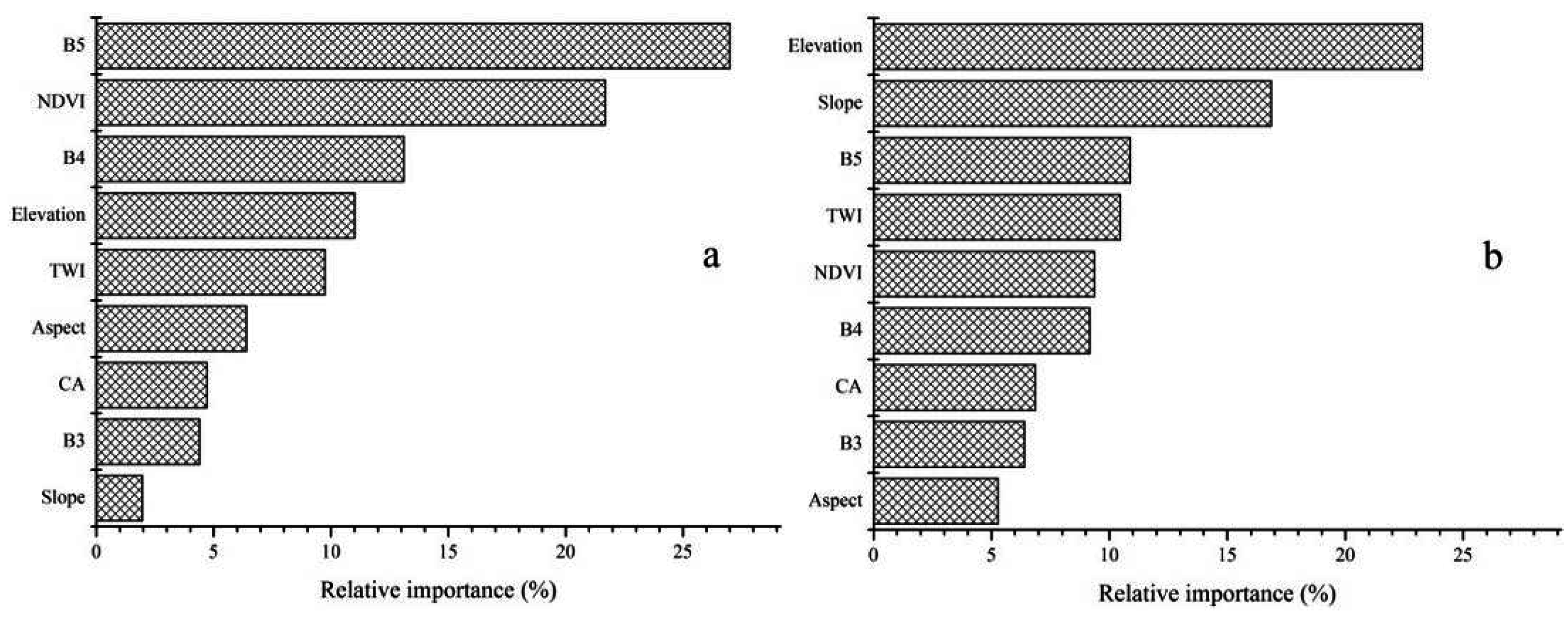
3.3. Relative Importance of Environmental Variables

Variable importance revealed different dominating environmental factors of SOC in 1990 and 2010 (Figure 5). RS indices were the primary variables influencing SOC in 1990, as it was topography in 2010 (Figure 5). In 1990, NDVI (RI > 20%) in both years showed high indicating ability of the topsoil organic carbon in coastal mountain areas. This finding is consistent with previous studies [22,55,56,57,58]. It implies that there is a potential of remote sensing in mapping SOC distribution in coastal mountain regions with humid climates. Minnasny et al. [59] reported that such indices were not only excellent predictors, but also played positive roles in the microbial activities in soils affecting the distribution of SOC.

The lower influence of NDVI on SOC in 2010 can be attributed to the heavy land-use change such as a large number of forests, grasslands and wetlands converted to agriculture from 1990 to 2010. Some studies [7,12,13] suggested that land-use change had a significant effect on SOC dynamics, since the start of the economic reforms in 1990 in Wafangdian City. This transformation weakened the intrinsic relationship between land-use and organic carbon. Yang et al. [22] concluded that band B3 had an excellent ability to predict SOC in high altitude areas (3200–3600 m). Surprisingly, our study found a lower relative importance of B3 in both periods. Although B3 was useful in distinguishing vegetation types and coverage, it showed the lowest importance. This is likely to be partly mediated by elevation and NDVI, which provide more detailed information in a landscape.

Topography has been recognized as one of the key pedogenetic factors influencing the distribution of SOC. In a high-variation of relief, topography was good predictors for mapping SOC [38,60]. We found topographic variables showed higher RI in 2010 (64% in 2010, and 34% in 1990). Elevation was identified as a key topographic factor in both periods. This is consistent with previous studies [60,61]. Altitude affects vegetation, local climate, and microbial activity, which have prolonged influence on SOC dynamics. TWI is related to soil moisture status, and it has been successfully used in predicting SOC in several studies [12,62,63,64]. Because of high variation in relief in the area, slope and aspect may have an effect on microclimate on local scales. We found that the influence of slope gradient was different in two periods (2% in 1990; 20% in 2010). In the study, the dataset of 1990 does not include samples in high slopes. This is because sampling is quite difficult in these areas. The purposive sampling strategy used in 2010 involving soil samples from those areas. The predictive model identified the substantial contribution of slope gradient on SOC distribution. Spatial visualization of results was essential to understand the driving forces on SOC distribution.

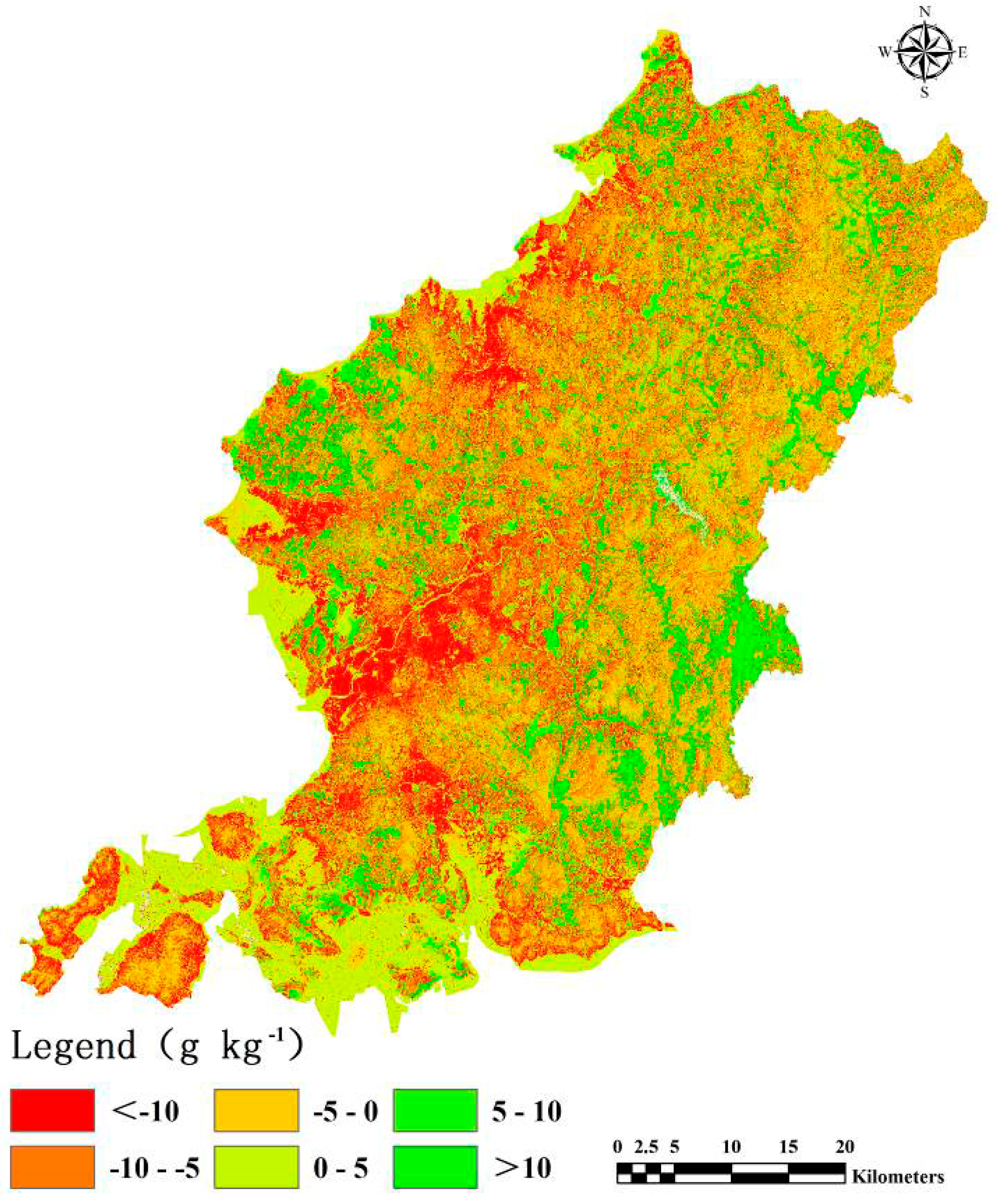
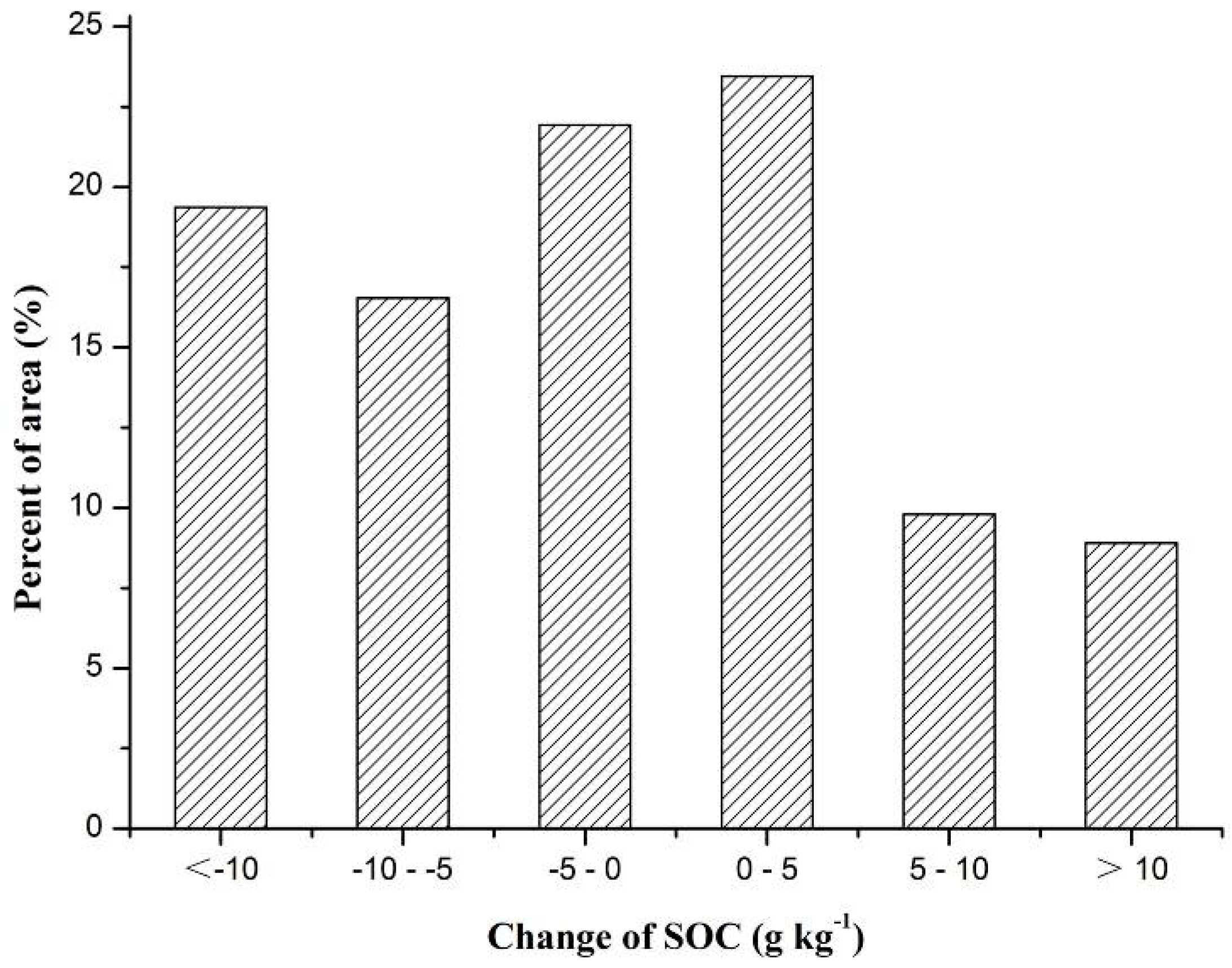
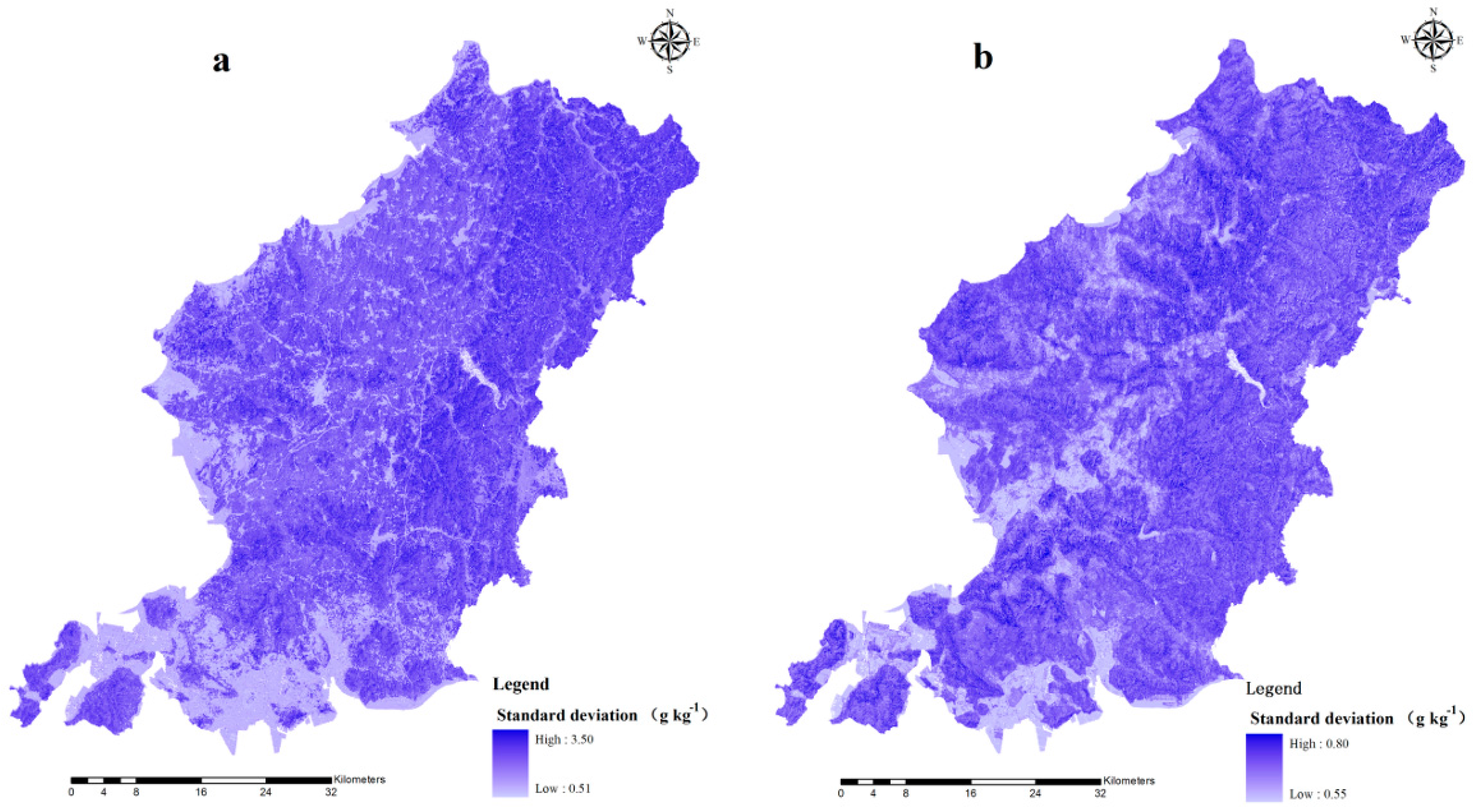
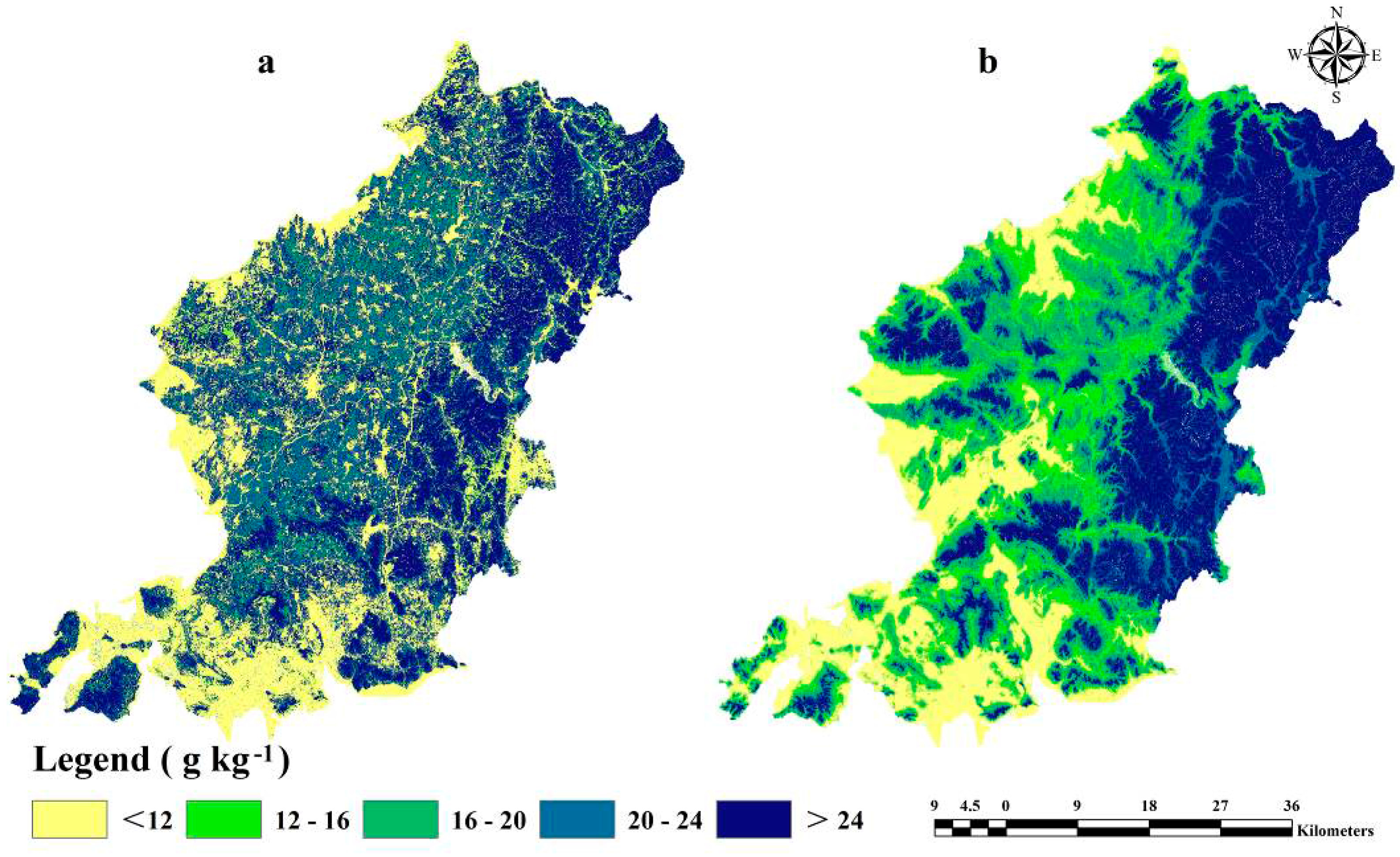
3.4. SOC Content Maps and Spatial-Temporal Changes

Figure 6 shows the predicted SOC in 1990 and 2010. They are means of 100 runs of BRT models. Average SOC content was higher in 1990 (20.8 ± 9.7 g∙kg⁻¹) than that in 2010 (18.6 ± 6.0 g∙kg⁻¹). The percentages of SOC content related to levels were shown in Figure 7. In both periods, SOC was high in the east and low in the southwest of Wafangdian City. High SOC content was observed in the regions covered with densely river network and forest. Spatial patterns of SOC content in 1990 were closely related to vegetation, which had been examined in recent studies [55,56,65,66]. This spatial pattern was closely related to elevation in 2010.

Based on cluster analysis, we obtained five grades of SOC content in two periods. In 1990, SOC content was mainly distributed at level E (>24 g∙kg⁻¹⁾, accounting for about 29% of the total area (Figure 7). The highest SOC content level (E) was mainly observed in the Mountain and Hilly Area of Eastern, and the lowest level (A) (<12 g∙kg⁻¹) was mainly associated with soils in western and southwestern parts of the coastal areas (Figure 6a).

In 2010, SOC content was mainly distributed at levels A (<12 g∙kg⁻¹) and E (>24 g∙kg⁻¹), accounting for 29% and 43% of the total study area (Figure 7). High SOC content was mainly distributed in the northeast mountainous area and eastern part of Wafangdian City; the low SOC content was mainly in the western parts of the low-hilly land and coastal plains (Figure 6b). From 1990 to 2010, SOC content was improved with the shift from levels B and C to levels A and E. The area of level A and E increased by 10% and 14%, respectively. The area of level B and C decreased by 12% and 13%.

Many studies revealed that land-use change had a significant effect on SOC content distribution [12,13]. Land use in Wafangdian City has undergone an intense change during the past decades, manifesting substantial consequences on SOC. Zhao et al. [10] reported an increased SOC level in all geographic areas of Jiangsu Province, China within a 26 year time period. Although there was a decreased trend in most parts of the study area, but few changes happened in the coastal plain. The area with SOC decreasing accounted for 58% of the total area mainly in the eastern mountainous (<−10 g∙kg⁻¹) and the central plains −5 to 0 g∙kg⁻¹ (Figure 8). The highest increase (>10 g∙kg⁻¹) occurred in the western and eastern plain, accounting for 9% of the total area (Figure 9). Increasing SOC (0 to 5 g∙kg⁻¹) content was mainly in the southwest coastal areas (28%). The highest decrease (−5 to 0 g∙kg⁻¹) appeared in the central part of plain and eastern mountainous regions, accounting for about 6% of the total area.

3.5. Effects of Land-Use Change on SOC Content

Land use has significant impacts on SOC by affecting soil properties and biomass production. Dramatic land-use change, such as shifts from forest to cultivation or grassland, resulted in a completely different soil environment in terms of soil moisture and temperature regimes. It significantly influenced organic matter accumulation and decomposition dynamics [6,64]. Zhao et al. [7] reported that soil organic matter (SOM) in about 26 year, when upland was changed to paddy field, had the largest increase of 5.41 ± 3.95 g k⁻¹ in Jiangsu Province of China.

Changes in SOC from 1990 to 2010 varied with changes in land use types. A substantial change in SOC was observed when there was no land use change as well. For example, soils in unchanged cultivated land in 1990 and 2010, we observed an average loss of −2.6 g∙kg⁻¹ SOC. Soils under unchanged forest and grassland also lost amounts of SOC from 1990 to 2010. These patterns showed a decreasing SOC trend when there was no change in land use. This could be attributed to a substantial amount of production and living activities with no increase in biomass inputs to soils.

In changed land-use types, averages of SOC change ranged from −1.6 g∙kg⁻¹ to −3.6 g∙kg⁻¹. The greatest change occurred when grassland was converted to cultivated land (G–C) and forest was converted to cultivated (F–C) (

Table 5. Change of SOC content under different land-use patterns during 1990–2010.

Land-Use Change	Change Range (g∙kg−1)	Mean ± SD
Cultivation–Cultivation (C–C)	−29.6 to 20.2	−2.6 ± 9.3
Cultivation–Forest (C–F)	−27.0 to 18.9	−1.6 ± 8.5
Cultivation–Grassland (C–G)	−24.0 to 18.9	−1.8 ± 9.7
Grassland–Grassland (G–G)	−23.0 to 18.9	−1.2 ± 7.9
Grassland–Cultivation (G–C)	−29.5 to 20.2	−3.6 ± 9.2
Grassland–Forest (G–F)	−26.5 to 19.7	−2.3 ± 8.7
Forest–Forest (F–F)	−28.7 to 20.3	−2.6 ± 9.0
Forest–Grassland (F–G)	−17.6 to 15.2	−1.6 ± 8.0
Forest–Cultivation (F–C)	−19.6 to 19.1	−2.5 ± 9.7

). The smallest change occurred in F–G (Forest land–Grassland). Land-use types that had been changed to grassland had considerable reduction in SOC content. For example, by shifting from forest to grassland, soil has changed from oxidation status to substitution oxidation-increase environment. It leads to a significant increase in the decomposition rate of soil organic matter (SOM) and a decline in the accumulation rate [7,8,9].

These results suggested that land use changes played various roles in SOC. In total, the area had experienced SOC declining from 1990 to 2010. This could be linked to the economic development of Wafangdian City during the 1980s, and the city size and population increased so rapidly that a large area of agricultural land was swallowed by construction areas. Ground vegetation was swapped and the areas were isolated from water recharge and gaseous exchange [11]. Such transformation caused a tremendous decline in SOC content (Table 2). The regions with steep SOC declines were mostly situated in the eastern mountain area, where most of the forest had been converted to apple, cherry or peach plantations. These changes have negative effects on SOC accumulation (Table 2). It was unexpected that the SOC content in the southwestern hilly area, where national farms dominate and land-use types had not changed greatly, did not show a substantial change during the past 20 years. In general, there was an overall decrease in SOC (Table 2 and Table 5) content but with decreasing rates from north to south of the Wafangdian City.

4. Conclusions

We identified the main factors driving spatial-temporal changes of topsoil organic carbon content at a regional scale in the northeast China. The spatial distributions of SOC content at two periods (1990 and 2010) were mapped by the BRT model. The results demonstrated that the BRT model is an effective and powerful tool for mapping spatial patterns of SOC content. Land-use changes caused by industrialization were the primary reasons that account for spatial-temporal changes of SOC content in the area. Variations in topography also played a key role in the spatial-temporal distribution of SOC content. Spatially, the distribution of SOC content had shown a decreasing trend from north to south between two periods. Remaining unchanged areas were located in the Low Mountain and Hilly Areas in the southwestern parts. Spatial-temporal changes of SOC content were influenced by rapid urbanization and land-use changes. Since the 1990s, land use has been severely changed such as agriculture lands converted to constructions in Wafangdian City. Because of the importance of SOC in regional carbon cycling and soil fertility, accurate spatial mapping of SOC content were essential for evaluating soil quality and carbon sequestration potential in Wafangdian City.

References

1. Batjes, N.H. Total carbon and nitrogen in the soils of the world. Eur. J. Soil Sci. 1996, 47, 151–163. [Google Scholar] [CrossRef]
2. Bohn, H.L. Estimate of organic carbon in world soils: II. Soil Sci. Soc Am. J. 1982, 46, 1118–1119. [Google Scholar] [CrossRef]
3. Grace, J. Understanding and managing the global carbon cycle. J. Ecol. 2004, 92, 189–202. [Google Scholar] [CrossRef]
4. Lal, R. Soil carbon sequestration to mitigate climate change. Geoderma 2004, 123, 1–22. [Google Scholar] [CrossRef]
5. Gal, A.; Vyn, T.J.; Micheli, E.; Kladivko, E.J.; McFee, W.W. Soil carbon and nitrogen accumulation with long-term no-till versus moldboard plowing overestimated with tilled-zone sampling depths. Soil Tillage Res. 2007, 96, 42–51. [Google Scholar] [CrossRef]
6. Wiesmeier, M.; Hübner, R.; Spörlein, P.; Geuß, U.; Hangen, E.; Reischl, A.; Schilling, B.; Lützow, M.; Kögel-Knabner, I. Carbon sequestration potential of soils in southeast Germany derived from stable soil organic carbon saturation. Glob. Chang. Biol. 2014, 20, 653–665. [Google Scholar] [CrossRef] [PubMed]
7. Zhao, M.S.; Zhang, G.L.; Wu, Y.J.; Li, D.C.; Zhao, Y.G. Driving forces of soil organic matter change in Jiangsu Province of China. Soil Use Manag. 2015, 31, 440–449. [Google Scholar] [CrossRef]
8. Mann, L.K. Changes in soil carbon storage after cultivation. Soil Sci. 1986, 142, 279–288. [Google Scholar] [CrossRef]
9. Paustian, K.; Andrén, O.; Janzen, H.H.; Lal, R.; Smith, P.; Tian, G.; Tiessen, H.; Van Noordwijk, M.; Woomer, P.L. Agricultural soils as a sink to mitigate CO2 emissions. Soil Use Manag. 1997, 13, 230–244. [Google Scholar] [CrossRef]
10. Cruz, F.T.; Pitman, A.J.; McGregor, J.L. Probabilistic simulations of the impact of increasing leaf-level atmospheric carbon dioxide on the global land surface. Clim. Dyn. 2010, 34, 361–379. [Google Scholar] [CrossRef]
11. Zhang, F.; Li, C.; Wang, Z.; Wu, H. Modeling impacts of management alternatives on soil carbon storage of farmland in Northwest China. Biogeosciences 2006, 3, 451–466. [Google Scholar] [CrossRef]
12. Yin, K.; Lu, D.S.; Tian, Y.C.; Zhao, Q.J.; Yuan, C. Evaluation of Carbon and Oxygen Balances in Urban Ecosystems Using Land Use/Land Cover and Statistical Data. Sustainability 2014, 7, 195–221. [Google Scholar] [CrossRef]
13. Qiu, L.F.; Zhu, J.X.; Wang, K.; Hu, W. Land Use Changes Induced County-Scale Carbon Consequences in Southeast China 1979–2020, Evidence from Fuyang, Zhejiang Province. Sustainability 2015, 8, 38. [Google Scholar] [CrossRef]
14. McBratney, A.B.; Mendonça Santos, M.L.; Minasny, B. On digital soil mapping. Geoderma 2003, 117, 3–52. [Google Scholar] [CrossRef]
15. Jenny, H. Factors of Soil Formation: A System of Quantitative Pedology; Beth, R., Ed.; Soil Science: Philadelphia, PA, USA, 1941; Volume 42, p. 415. [Google Scholar]
16. Zhao, M.S.; Rossiter, D.G.; Li, D.C.; Zhao, Y.G.; Yang, J.L.; Liu, F.; Zhang, G.L. Mapping soil organic matter in low-relief areas based on land surface diurnal temperature difference and a vegetation index. Ecol. Indic. 2014, 39, 120–133. [Google Scholar] [CrossRef]
17. Brus, D.J.; Yang, R.M.; Zhang, G.L. Three-dimensional geostatistical modeling of soil organic carbon: A case study in the Qilian Mountains, China. Catena 2016, 141, 46–55. [Google Scholar] [CrossRef]
18. Marvin, D.C.; Asner, G.P.; Schnitzer, S.A. Liana canopy cover mapped throughout a tropical forest with high-fidelity imaging spectroscopy. Remote Sens. Environ. 2016, 176, 98–106. [Google Scholar] [CrossRef]
19. Grimm, R.; Behrens, T.; Märker, M.; Elsenbeer, H. Soil organic carbon concentrations and stocks on Barro Colorado Island-digital soil mapping using Random Forests analysis. Geoderma 2008, 146, 102–113. [Google Scholar] [CrossRef]
20. Yang, R.M.; Zhang, G.L.; Liu, F.; Lu, Y.Y.; Yang, F.; Yang, F.; Yang, M.; Zhao, Y.G.; Li, D.C. Comparison of boosted regression tree and random forest models for mapping topsoil organic carbon concentration in an alpine ecosystem. Ecol. Indic. 2016, 60, 870–878. [Google Scholar] [CrossRef]
21. Wiesmeier, M.; Barthold, F.; Blank, B.; Kögel-Knabner, I. Digital mapping of soil organic matter stocks using Random Forest modeling in a semi-arid steppe ecosystem. Plant Soil 2011, 340, 7–24. [Google Scholar] [CrossRef]
22. Were, K.; Bui, D.T.; Dick, Ø.B.; Singh, B.R. A comparative assessment of support vector regression, artificial neural networks, and random forests for predicting and mapping soil organic carbon stocks across an Afromontane landscape. Ecol. Indic. 2015, 52, 394–403. [Google Scholar] [CrossRef]
23. Minasny, B.; Setiawan, B.I.; Arif, C.; Saptomo, S.K.; Chadirin, Y. Digital mapping for cost-effective and accurate prediction of the depth and carbon stocks in Indonesian peatlands. Geoderma 2016, 272, 20–31. [Google Scholar]
24. Froeschke, J.T.; Froeschke, B.F. Spatio-temporal predictive model based on environmental factors for juvenile spotted seatrout in Texas estuaries using boosted regression trees. Fish. Res. 2011, 111, 131–138. [Google Scholar] [CrossRef]
25. Adhikari, K.; Kheir, R.B.; Greve, M.B.; Greve, M.H. Comparing kriging and regression approaches for mapping soil clay content in a diverse Danish landscape. Soil Sci. 2013, 178, 505–517. [Google Scholar] [CrossRef]
26. Skurichina, M.; Duin, R.P. Bagging, boosting and the random subspace method for linear classifiers. Pattern Anal. Appl. 2002, 5, 121–135. [Google Scholar] [CrossRef]
27. Elith, J.; Leathwick, J.R.; Hastie, T. A working guide to boosted regression trees. J. Anim. Ecol. 2008, 77, 802–813. [Google Scholar] [CrossRef] [PubMed]
28. Friedman, J.H.; Meulman, J.J. Multiple additive regression trees with application in epidemiology. Stat. Med. 2003, 22, 1365–1381. [Google Scholar] [CrossRef] [PubMed]
29. Minasny, B.; McBratney, A.B.; Mendonça-Santos, M.L.; Odeh, I.O.A.; Guyon, B. Prediction and digital mapping of soil carbon storage in the Lower Namoi Valley. Aust. J. Soil Res. 2006, 44, 233–244. [Google Scholar] [CrossRef]
30. Pouteau, R.; Rambal, S.; Ratte, J.P.; Gogé, F.; Joffre, R.; Winkel, T. Downscaling MODIS-derived maps using GIS and boosted regression trees: the case of frost occurrence over the arid Andean highlands of Bolivia. Remote Sens. Environ. 2011, 115, 117–129. [Google Scholar] [CrossRef]
31. Carslaw, D.C.; Taylor, P.J. Analysis of air pollution data at a mixed source location using boosted regression trees. Atmos. Environ. 2009, 43, 3563–3570. [Google Scholar] [CrossRef]
32. Dhingra, M.S.; Dissanayake, R.; Negi, A.B.; Oberoi, M.; Castellan, D.; Thrusfield, M.; Linard, C.; Gilbert, M. Spatio-temporal epidemiology of highly pathogenic avian influenza (subtype H5N1) in poultry in eastern India. Spat. Spatio-Tempor. Epidemiol. 2014, 11, 45–57. [Google Scholar] [CrossRef] [PubMed]
33. Schad, P.; Van Huyssteen, C.; Micheli, E. International Soil Classification System for Naming Soils and Creating Legends for Soil Maps; World Reference Base for Soil Resources: Rome, Italy, 2014; Volume 106, pp. 246–385. [Google Scholar]
34. Zhu, A.X.; Yang, L.; Li, B.; Qin, C.; English, E.; Burt, J.E.; Zhou, C.H. Purposive sampling for digital soil mapping for areas with limited data. In Digital Soil Mapping with Limited Data; Hartemink, A.E., McBratney, A.B., de Lourdes, M.-S., Eds.; Springer: Amsterdam, The Netherlands, 2008; Volume 8, pp. 233–245. [Google Scholar]
35. Nelson, D.W.; Sommers, L.E. Methods of soil analysis. In Total Carbon, Organic Carbon, and Organic Matter, 2nd ed.; Miller, R.H., Keeney, D.R., Eds.; The Alliance of Crop, Soil, and Environmental Science Societies: Madison, WI, USA, 1982; Volume 2, pp. 539–579. [Google Scholar]
36. Olaya, V.F. A Gentle Introduction to Saga GIS; The SAGA User Group eV: Göttingen, Germany, 2004. [Google Scholar]
37. Gao, Y.Y.; Hua, H.M.; Wang, S.H.; Li, B. A fast image dehazing algorithm based on negative correction. Signal Process. 2014, 103, 380–398. [Google Scholar] [CrossRef]
38. Malone, B.P.; McBratney, A.B.; Minasny, B.; Laslett, G.M. Mapping continuous depth functions of soil carbon storage and available water capacity. Geoderma 2009, 154, 138–152. [Google Scholar] [CrossRef]
39. Friedman, J.; Hastie, T.; Tibshirani, R. Additive logistic regression: a statistical view of boosting. Ann. Stat. 2000, 28, 337–407. [Google Scholar] [CrossRef]
40. Liu, J.T.; Sui, C.H.; Deng, D.W.; Wang, J.W.; Feng, B.; Liu, W.Y.; Wu, C.H. Representing conditional preference by boosted regression trees for recommendation. Inf. Sci. 2016, 327, 1–20. [Google Scholar] [CrossRef]
41. Saha, D.; Alluri, P.; Gan, A. Prioritizing Highway Safety Manual’s crash prediction variables using boosted regression trees. Accid. Anal. Prev. 2015, 79, 133–144. [Google Scholar] [CrossRef] [PubMed]
42. Martin, M.P.; Wattenbach, M.; Smith, P.; Meersmans, J.; Jolivet, C.; Boulonne, L.; Arrouays, D. Spatial distribution of soil organic carbon stocks in France. Biogeosciences 2011, 8, 1053–1065. [Google Scholar] [CrossRef] [Green Version]
43. Müller, D.; Leitão, P.J.; Sikor, T. Comparing the determinants of cropland abandonment in Albania and Romania using boosted regression trees. Agric. Syst. 2013, 117, 66–77. [Google Scholar] [CrossRef]
44. Dismo: Species Distribution Modeling, R Package Version 0.8-17. Available online: http://dssm.unipa.it/CRAN/web/packages/dismo/ (accessed on 31 December 2013).
45. Gbm: Generalized Boosted Regression Models, R Package Version 1.6-3. Available online: http://127.0.0.1:31000/library/gbm/html/gbm-package.html (accessed on 26 November 2007).
46. Yoon, L.C.; Pedro, J.; Leitão, T.L. Assessment of land use factors associated with dengue cases in Malaysia using Boosted Regression Trees. Spat. Spatio-Tempor. Epidemiol. 2014, 10, 75–84. [Google Scholar]
47. Oksanen, J.; Kindt, R.; Legendre, P.; Oksanen, M.J. Vegan: Community Ecology Package, version 1.15-4; R Foundation for Statistical Computing: Vienna, Austria, 2014; Volume 3, pp. 1–13. [Google Scholar]
48. Lin, L. A concordance correlation coefficient to evaluate reproducibility. Biometrics 1989, 45, 255–268. [Google Scholar] [CrossRef] [PubMed]
49. Ließ, M.; Glaser, B.; Huwe, B. Uncertainty in the spatial prediction of soil texture: comparison of regression tree and Random Forest models. Geoderma 2012, 170, 70–79. [Google Scholar] [CrossRef]
50. Razakamanarivo, R.H.; Grinand, C.; Razafindrakoto, M.A.; Bernoux, M.; Albrecht, A. Mapping organic carbon stocks in eucalyptus plantations of the central highlands of Madagascar: A multiple regression approach. Geoderma 2011, 162, 335–346. [Google Scholar] [CrossRef]
51. Guo, L.B.; Gifford, R.M. Soil carbon stocks and land use change: A meta-analysis. Glob. Chang. Biol. 2002, 8, 345–360. [Google Scholar] [CrossRef]
52. Bowman, R.A.; Reeder, J.D.; Wienhold, B.J. Quantifying laboratory and field variability to assess potential for carbon sequestration. Commun. Soil Sci. Plant Anal. 2002, 33, 1629–1642. [Google Scholar] [CrossRef]
53. Goidts, E.; Van Wesemael, B.; Crucifix, M. Magnitude and sources of uncertainties in soil organic carbon (SOC) stock assessments at various scales. Eur. J. Soil Sci. 2009, 60, 723–739. [Google Scholar] [CrossRef]
54. Krishnan, P.; Bourgeon, G.; Lo Seen, D.; Nair, K.M.; Prasanna, R.; Srinivas, S.; Muthusankar, G.; Dufy, L.; Ramesh, B.R. Organic carbon stock map for soils of southern India: a multifactorial approach. Curr. Sci. 2007, 93, 706–710. [Google Scholar]
55. Yang, Y.H.; Fang, J.Y.; Tang, Y.H.; Ji, C.J.; Zheng, C.Y.; He, J.S.; Zhu, B. Storage, patterns and controls of soil organic carbon in the Tibetan grasslands. Glob. Chang. Biolog. 2008, 14, 1592–1599. [Google Scholar] [CrossRef]
56. Shi, Y.; Baumann, F.; Ma, Y.; Song, C.; Kühn, P.; Scholten, T.; He, J.S. Organic and inorganic carbon in the topsoil of the Mongolian and Tibetan grasslands: pattern, control and implications. Biogeosciences 2012, 9, 2287–2299. [Google Scholar] [CrossRef]
57. Riano, D.; Chuvieco, E.; Salas, J.; Aguados, I. Assessment of different topographic corrections in Landsat-TM data for mapping vegetation types. IEEE Trans. Geosci. Remote Sens. 2003, 41, 1056–1061. [Google Scholar] [CrossRef]
58. Geerken, R.; Zaitchik, B.; Evans, J.P. Classifying rangeland vegetation type and coverage from NDVI time series using Fourier Filtered Cycle Similarity. Int. J. Remote Sens. 2005, 26, 5535–5554. [Google Scholar] [CrossRef]
59. Minasny, B.; McBratney, A.B.; Malone, B.P.; Wheeler, I. Digital mapping of soil carbon. Adv. Agron. 2013, 118, 1–47. [Google Scholar]
60. Romano, N.; Palladino, M. Prediction of soil water retention using soil physical data and terrain attributes. J. Hydrol. 2002, 265, 56–75. [Google Scholar] [CrossRef]
61. Thompson, J.A.; Bell, J.C.; Butler, C.A. Quantitative Soil-Landscape Modeling for Estimating the Areal Extent of Hydromorphic Soils. Soil Sci. Soc. Am. J. 1997, 61, 971–980. [Google Scholar] [CrossRef]
62. Adhikari, K.; Hartemink, A.E.; Minasny, B.; Bou Kheir, R.; Greve, M.B.; Greve, M.H. Digital Mapping of Soil Organic Carbon Contents and Stocks in Denmark. PLoS ONE 2014, 9, e105519. [Google Scholar] [CrossRef] [PubMed]
63. Moore, I.D.; Gessler, P.E.; Nielsen, G.A.; Peterson, G.A. Soil Attribute Prediction Using Terrain Analysis. Soil Sci. Soc. Am. J. 1993, 57, 443–452. [Google Scholar] [CrossRef]
64. Wiesmeier, M.; Barthold, F.; Spörlein, P.; Geuß, U.; Hangen, E.; Reischl, A.; Schilling, B.; Angst, G.; Von Lützow, M.; Kögel-Knabner, I. Estimation of total organic carbon storage and its driving factors in soils of Bavaria (southeast Germany). Geod. Reg. 2014, 1, 67–78. [Google Scholar] [CrossRef]
65. Jobbágy, E.G.; Jackson, R.B. The vertical distribution of soil organic carbon and its relation to climate and vegetation. Ecol. Appl. 2000, 10, 423–436. [Google Scholar] [CrossRef]
66. Jin, X.M.; Wan, L.; Zhang, Y.K.; Hu, G.C.; Schaepman, M.E.; Clevers, J.G.P.W.; Su, Z. Quantification of spatial distribution of vegetation in the Qilian Mountain area with MODIS NDVI. Int. J. Remote Sens. 2009, 30, 5751–5766. [Google Scholar] [CrossRef]
Figure 1. Location of sampling sites in the study area.
Sustainability 08 01154 g001
Figure 2. Geographic areas map of Wafangdian City.
Sustainability 08 01154 g002
Figure 3. Boxplot of SOC content in 1990 and 2010 derived for different environmental variables. SOC, Soil Organic Carbon; TWI, topographic wetness index; CA, catchment area; B3, Landsat TM band 3; B4, Landsat TM band 4; B5, Landsat TM band 5; NDVI, Normalized Difference Vegetation Index; and SD, Standard deviation.
Sustainability 08 01154 g003
Figure 4. Standard deviation of SOC predicted by the BRT model in the (a) 1990 and (b) 2010 surveys. BRT, boosted regression trees.
Sustainability 08 01154 g004
Figure 5. Relative importance of each variable as determined from 100 runs of the boosted regression trees (BRT) in 1990 (a) and 2010 (b) surveys, which are shown in decreasing order and normalized to 100%. TWI, SAGA wetness index; CA, catchment area; B3, Landsat TM band 3; B4, Landsat TM band 4; B5, Landsat TM band 5; NDVI, Normalized Difference Vegetation Index.
Sustainability 08 01154 g005
Figure 6. Mean spatial distribution maps of SOC content predicted by the BRT model in (a) 1990 and (b) 2010 surveys.
Sustainability 08 01154 g006
Figure 7. Area percentages of different SOC content levels and changes in 1990 and 2010 surveys; levels A < 12 g∙kg−1, 12 g∙kg−1 < levels B < 16 g∙kg−1, 16 g∙kg−1 < levels C < 20 g∙kg−1, 20 g∙kg−1 < levels D < 24 g∙kg−1, levels E >24 g∙kg−1.
Sustainability 08 01154 g007
Figure 8. Spatial distributions of SOC change between the1990 and 2010 surveys.
Sustainability 08 01154 g008
Figure 9. Area percentages of SOC change at different levels between 1990 and 2010 surveys.
Sustainability 08 01154 g009