Abstract
This paper presents a game-theoretical analysis of joint decisions on carbon emission reduction and inventory replenishment with overconfidence and consumer’s low-carbon preference for key supply chain players when facing effort-dependent demand. We consider respectively the overconfidence of a supplier who overestimates the impacts of his emission reduction efforts on product demand and the overconfidence of a retailer who underestimates the variability of the stochastic demand. We find, surprisingly, that the supplier’s overconfidence can mitigate “double marginalization” but hurt self-profit, while the retailer’s overconfidence can be an irrelevant factor for self-profit. The retailer aiming at short-term trading should actively seek an overconfident supplier, while the supplier should actively seek a rational retailer for whom the critical fractile is more than 0.5, whereas for an overconfident retailer, the critical fractile is less than or equal to 0.5. The study also underlines the effect of regulation parameters as an important contextual factor influencing low-carbon operations.
1. Introduction
The high-carbon economy, dominated by fossil fuels, leads to serious environmental problems around the world, especially air pollution. China is a prime example. The Global Burden of Disease Study (GBD 2013) of the World Health Organization (WHO) forecasts that air pollution will lead to 1.3 million premature deaths and more than 27 million years of life lost each year at the beginning of 2030 in China [1]. Under such a harsh environment, many customers’ preference has turned to ‘low-carbon’ products. For example, the general public prefers organic food, green furnishings, and products from companies with favorable images. A study carried out by European Commission in 2008 shows that 75% of Europeans are ready to buy costlier green products, compared to 31% in 2005, and 72% of consumers support “carbon labels” [2]. In this context, there is a growing number of suppliers participating in carbon emission reduction, energy efficiency improvement, and green materials usage.
Over the past few years, substantial effort by responsible firms has been made to reduce carbon emissions. Some firms optimize their operation process to improve energy efficiency [3,4,5], and some invest in cleaner technologies to achieve low-carbon manufacturing [6,7,8]. In practice, Walmart designs and opens low-carbon supermarkets [9]; Siemens supports its supplier to reduce energy consumption [10]; H&M adopts new technologies and launches the green label products [11]; Quanyou Household, a Chinese company which received the “International Green Design Award” in 2012, invests in environmentally friendly materials and equipment to reduce carbon emissions, and produces sustainable products [12]. Recent research focuses on the emission reduction decision and inventory policy. For instance, Benjaafar et al. [13] integrated the carbon emission concerns into the simple supply chain system for the first time and found that inventory optimization can remarkably reduce emissions without considerably increasing cost. Chen et al. [14] derived a condition under which a change in replenishment quantity can significantly reduce emissions without obviously increasing costs and interval range, in which the decrement of emissions is more than the increment of costs. Toptal et al. [15] found that carbon emission reduction investment, additional to reducing emissions as per regulations, further reduce carbon emissions while reducing costs. Żuchowski [16] put forward sustainable solutions to reduce emissions, consequently, in the long run, leading to a “green” warehouse. Chen et al. [17] analysed the impact of emission reduction investment on the warehouse management decisions and performances.
In addition, considering the emission reduction decision driven by consumer’s low-carbon preference has gradually become a hotspot, for example, it has been found [18,19,20,21,22] that the higher the consumer’s low-carbon preference, the more the consumers were willing to pay for eco-friendly products. As a result, the supplier is willing to win customers by reducing emissions. Other studies [12,23,24,25] also argued that the emission reduction decision is driven by consumer’s low-carbon preference. Swami and Shah [26] argued that the ratio of the optimal emission reduction efforts put in by the manufacturer and the retailer is equal to the ratio of their emission reduction sensitivity ratios and emission reduction cost ratios. Du et al. [27] found that the channel profit as well as emission reduction increases in consumer’s low-carbon preference simultaneously in particular cases. Dong et al. [11] examined the emission reduction level of the manufacturer and order quantity of the retailer and found that the order quantity may be increasing in the wholesale price due to the effect of low-carbon emission consideration.
However, most of these studies with effort-dependent demand are based on the assumption of rational agents. In reality, especially in complex and uncertain environments, decision makers tend to believe that their information or their estimates are more accurate than they actually are, namely that they are overconfident [28]. People, even experts, are prevalently overconfident in their estimations of random outcomes [29,30]. Hambrick [31] suggested that the behavioural characteristics of decision makers matter for organizational performance, thereby extending to operational activities such as inventory and ordering decisions. Other studies [32,33,34,35,36] have also confirmed that overconfidence is one of the most consistent, powerful, and widespread behavioural characteristics of decision makers in situations characterized by random outcome, both in field studies and controlled experiments. In field studies, Croson et al. [34] showed that overconfidence leads the newsvendor to place suboptimal orders and earn lower profits than well-calibrated newsvendors; Bendoly et al. [33] argued that overconfidence may lead purchasing managers to under-estimate the variance of demand or of lead-time, thus inducing them to hold too little safety stock. In controlled experiments, Ancarani et al. [32] evidenced that overconfidence leads to worse performance in inventory management; by contrast, Li et al. [37] found that overconfidence can potentially be a positive force. We extend these studies by incorporating the notion of overconfidence as a cognitive bias into a low-carbon supply chain system and find that, contrary to intuitive reasoning, the retailer’s performance is independent of his overconfidence.
As reviewed above, the existing literature have primarily examined joint decisions on carbon emission reduction and inventory management driven by consumer’s low-carbon preference. However, the research regarding how the consumer’s low-carbon preference and overconfidence of decision makers simultaneously affect emission reduction is never seen, which is very important for solving the operation decision problems, i.e., the impacts of supply chain agents’ deviation from rationality in decision on low-carbon operation. In this paper, hereby, we focus on joint decisions on carbon emission reduction and inventory replenishment with overconfidence and low-carbon preference. Under the condition of effort-dependent demand, such overconfidence may significantly affect emission reduction decision and the performance of all parties. Therefore, we incorporate both overconfidence of decision makers and consumer’s low-carbon preference into the general newsvendor model under four different scenarios: integrated SC (supply chain), decentralized SC, decentralized SC with an overconfident supplier, and decentralized SC with an overconfident retailer. In the extended cases, we further take various carbon policies into account when the supplier faces overconfidence. In particular, we provide insights to three important SC issues:
- How does overconfidence affect emission reduction and replenishment decisions when consumer’s low-carbon preference is taken into account?
- Could the supplier’s overconfidence hurt self-profit, and retailer’s?
- How do various carbon policies affect the optimal decisions and further affect carbon emissions of the supply chain?
The differences between our work and the work in related literature are:
- We simultaneously integrate the consumer’s low-carbon preference and overconfidence of decision makers into the joint decisions process of carbon emission reduction and inventory replenishment, and thus explore the deviation from supply chain operation caused by both.
- With demand sensitive to emission and following normal distribution, we analytically explore the effects of overconfidence on the unbiased equilibrium results, including supplier’s overconfidence that biases the demand scale and retailer’s overconfidence that biases the random demand variance, but not it’s mean.
- Contrary to commonly held beliefs, this result implies that the retailer’s performance is independent of the degree of his overconfidence.
The rest of this paper is organized as follows. Section 2 examines problem characteristics, formulates the game-theoretical models, and derives optimal solutions for four decision scenarios. Section 3 compares the equilibrium results among different settings and provides managerial insights. Section 4 extends the model of Scenario 3 with various carbon policies. Section 5 presents numerical analyses to further give more management insights. Section 6 concludes the study. Some proofs are relegated to the “Appendix”.
2. Problem Characteristics and Model Formulation
2.1. Problem Characteristics and Assumptions
In this paper, we consider a two-stage supply chain system composed of one supplier and one retailer. The supplier (denoted as s) provides a type of product in a make-to-order setting and sells them to customers in the end market by the aid of a retailer (denoted as r). The supplier is the main carbon emitter who contributes to the carbon footprint of the final product. Under the environmental support restrictions, the supplier invests in green technology to reduce carbon emissions during production and operation. In general, an increase in carbon reduction investment can effectively reduce the unit product carbon emissions, and in turn, for the customers with low-carbon preference, an increase in the level of carbon emission reduction effort can result in greater market demand. However, the level of emission reduction cannot increase infinitely and should be determined by the firms themselves. Hence, it is reasonable to assume that market demand is affected by both retail price and the level of emission reduction . We address two types of overconfidence: one is that the supplier overestimates the impacts of his emission reduction efforts on product demand, overconfidence factor is ; the other one is that the retailer underestimates the variability of the stochastic demand, overconfidence factor is . We capture the impacts of supplier’s overconfidence, retailer’s overconfidence, and consumer’s low-carbon preference on the supplier’s emission reduction efforts, retailer’s replenishment quantity, and profitability of supply chain players.
The following assumptions are considered in developing our mathematical models:
Assumption 1.
The level of emission reduction satisfies and , i.e., the higher the carbon reduction investment, the more effort the supplier exerts, but marginal investment has diminishing return in efforts.
Assumption 2.
Similar to the way as in [38,39], we assume that both product wholesale price and retail price are constant in order to concentrate on the key problem, and set .
Assumption 3.
One party of the supply chain is fully rational if the other is overconfident, i.e., when , and when . and are exogenous parameters.
Assumption 4.
The retailer faces stochastic demand for product, is a random factor following a normal distribution, a mean value of , a standard deviation value of , and in the range of , . The probability density function (PDF) and cumulative distribution function (CDF) of are and , respectively.
2.2. Model Formulation and Solution
In this section, we will first determine the demand function with consumer’s preference to low carbon and the investment cost function with emission reduction efforts, then characterize the supplier’s overconfidence and retailer’s overconfidence.
Supposing the market demand function the retailer faced follows an additive form defined as , and is the determined part of the demand function as the mean demand, coefficient reflects the consumer’s sensitiveness and preference level on low-carbon emission, and denotes the effort level of emission reduction. is the random part of the demand function as a random variable.
When consumers have low-carbon preference, the market demand of a product increases with supplier’s carbon emission reduction investment. Similar to the literature [8], we assume that supplier’s emission reduction investment cost is a concave increasing function regarding the emission reduction level , as shown in Figure 1. Constrained by the current technological level of carbon reduction, it is believed that the supplier cannot get carbon emission free by reducing all of his emissions, therefore the emission reduction level should satisfy , . Therefore, we denote the carbon reduction investment as a quadratic function of the emission reduction level, i.e., .
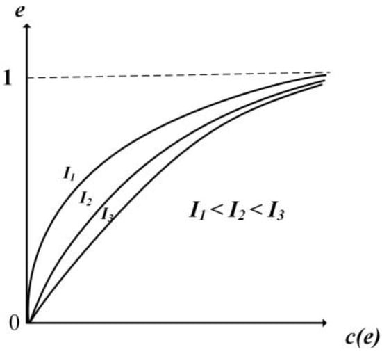
Figure 1.
Emission-reduction effort function.
With an overconfident supplier–rational retailer, the supplier overestimates the impacts of his emission reduction efforts on market demand. The overestimated demand function can be expressed as , where larger implies more overconfidence. . The PDF and CDF of are and , respectively. With a rational supplier–overconfident retailer, the retailer underestimates the variability of the stochastic demand. The underestimated demand function can be expressed as , , where smaller implies more overconfidence. The PDF and CDF of are and , respectively.
Considering all the model assumptions, the supplier’s, retailer’s, and the overall supply chain’s profit functions are given as:
2.2.1. Scenario 1: Centralized Model
In this section, we consider a centralized system, where a central decision maker (the supplier, the retailer, or a third party) wishes to seek the optimal decision set (the effort level of emission reduction and replenishment quantity) of perfect equilibria of the whole supply chain.
Note that Equation (3) is similar to the classic newsvendor model, so we can easily obtain optimal effort level of emission reduction and replenishment quantity.
2.2.2. Scenario 2: Decentralized Model
In a decentralized supply chain system, the supplier moves first and decides the effort level of emission reduction to maximize his own profit based on the demand information. Then the retailer moves sequentially on the basis of the supplier's decision, will decide whether to accept or not, make plans on replenishment, and place orders to the supplier so as to maximize his profit. This is a typical complete information dynamic game in which the supplier acts as a Stackelberg leader and the retailer acts as a follower.
We employ the standard backward induction to solve the dynamic game described above. In the second game step, we solve the retailer’s expected profit function under the condition that the supplier’s emission reduction efforts are given. We obtain the optimal response function of the replenishment quantity by maximizing Equation (1).
Substituting Equation (6) into Equation (2), we get the optimal emission reduction efforts in the decentralized decision by the first- and second-order conditions.
Substituting Equation (7) into Equation (6) yields the optimal replenishment quantity in the decentralized decision.
① Scenario 3: When the supplier is overconfident of future demand
With an overconfident supplier–rational retailer, the demand function is . According to the stocking factor method proposed by [40], we similarly define a auxiliary variable , represented stocking factor, as
Faced with Equation (1), the retailer’s expected profit function can be changed equivalently to
On the basis of Equation (10), the optimal response function of the replenishment quantity is
Similarly, substituting Equation (11) into Equation (2), we get the optimal emission reduction efforts denoted as
In fact, Equation (11) is a mathematical projection, not the actual response function of the retailer. Due to the assumption that the retailer is the follower and fully rational, when the supplier is overconfident, the actual response function of the retailer should be according to Equation (6). Therefore, the optimal replenishment quantity is
② Scenario 4: When the retailer is overconfident of future demand
With a rational supplier–overconfident retailer, the demand function is . Similarly, Equation (1) takes the following form
Faced with Equation (14), the optimal response function of the replenishment quantity is
Similarly, substituting Equation (15) into Equation (2), we get the optimal emission reduction efforts denoted as
Substituting Equation (16) into Equation (15) yields the optimal replenishment quantity denoted as
3. Game Equilibrium Analysis
Here, we compare the equilibrium results derived in the previous section and summarize the key findings and insights on the research.
Proposition 1.
If , then ; if , then is always true.
Proof.
From Equations (5) and (12), we can obtain , so has a threshold , i.e., when , and when . From Equations (5) and (7), we get , and incorporating the assumption , we find . Similarly, from Equations (7) and (12), we get , and incorporating the assumption and , we find . According to Equations (7) and (16), we obtain when .
This completes the proof. ☐
Proposition 1 shows that supplier’s overconfidence prompts the supplier to exert more effort on emission reduction, i.e., . According to the expression , is increasing in , and when increase to a certain threshold, emission reduction effort even exceeds that of the centralized decision, i.e., . There is no effect of the supplier’s emission reduction effort from retailer’s confidence in a rational supplier–overconfident retailer decentralized scenario, due to the assumption that the supplier is the leader and fully rational. Thus, the optimal emission reduction effort is the same as the case of decentralized model with a rational supplier–rational retailer, i.e., .
Proposition 2.
(i) In the decentralized model with an overconfident supplier–rational retailer, the optimal replenishment quantity rises as supplier’s overconfidence factor increases and . (ii) In the decentralized model with a rational supplier–overconfident retailer, when , the optimal replenishment quantity rises as retailer’s overconfidence factor falls and . However, when , the optimal replenishment quantity falls as decreases and .
From Proposition 1, we know that supplier’s emission reduction effort rises as his overconfidence factor increases in the decentralized decision with an overconfident supplier–rational retailer, which further adds demand. In the absence of emission-reduction cost sharing, the retailer would choose a higher replenishment quantity to gain more profits, thus we have ; under decentralized decision with a rational supplier–overconfident retailer, the smaller (), the smaller the variability of the stochastic demand, according to the ““ criterion of normal distribution, which corresponds to a smaller feasible interval of demand and greater probability of the random variable being equal to the mean , as shown in Figure 2. The ratio is called the critical fractile. When , i.e., , the market is in a low-profit condition, retailer’s replenishment quantity rises as falls and corresponding to or in Figure 2; when , i.e., , the market is in a high-profit condition, retailer’s replenishment quantity falls as decreases and corresponding to or in Figure 2. This means that the smaller , the more eager the retailer is to get his replenishment quantity clear to the expected demand, in order to hedge the risk from underestimating of demand fluctuation.
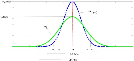
Figure 2.
Probability density distribution of the random variable.
Proposition 3.
In the decentralized model with an overconfident supplier–rational retailer, the retailer’s profit increases and the supplier’s profit decreases with supplier’s overconfidence factor .
When the supplier is overconfident of future demand, he will overestimate the effects of his emission-reduction efforts on product demand. According to Proposition 1, increasing in will stimulate the supplier to exert more emission-reduction efforts, which further results in a carbon emission reduction overinvestment, as a result, the supplier’s profit will be hurt by his own overconfidence eventually. However, it is good for the retailer, as the retailer does not need to bear the emission reduction investment cost but benefits from the expansion effect of low-carbon products on market demand. In reality, the retailer is more likely to seek an overconfident supplier or mislead the supplier’s cognition through distorting the demand information to achieve his free-riding.
Proposition 4.
In the decentralized model with a rational supplier–overconfident retailer, the supplier’s profit increases at for , and decreases at for , however, the retailer’s profit is independent of his overconfidence factor .
Proof.
Substituting Equations (16) and (17) into Equation (2), we can obtain
Due to , we have , where . According to the properties of the CDF, we know that when , so and the supplier’s profit increases at , similarly, when , so and the supplier’s profit decreases at .
Substituting Equations (16) and (17) into Equation (1), we can obtain
where , so and the retailer’s profit is independent of his overconfidence factor .
This completes the proof. ☐
When the retailer is overconfident of future demand, he will underestimate the variability of the stochastic demand. According to Proposition 2, when , the retailer will make his replenishment quantity increase as rises, which may make the supplier’s profit rise with the wholesale price and marginal production cost being constant; however, when , the retailer will make his replenishment quantity decrease as rises, which may make the supplier’s profit decline.
The retailer’s profit has no relation with his overconfidence factor , whether it is increasing or decreasing. The reason to this phenomenon may be: initial replenishment quantity from a rational retailer, due to his replenishment experience and information forecast, is already quite close to the actual market demand, however, an overconfident retailer tends to make replenishment quantity over-increased () or over-decreased () with respect to the overconfidence factor changing. When the replenishment quantity after increasing is more than the actual demand, the sale revenue, ordering cost, and holding cost increase, and the shortage cost decreases; when the replenishment quantity after decreasing is less than the actual demand, the sale revenue, ordering cost and holding cost decrease, and the shortage cost increases. The neutralization of revenues and costs results in that the retailer’s profit is independent of his overconfidence factor. What we find here is entirely different from those results in [32,35,36,37], which further enriches the related research involving overconfidence and low-carbon supply chain.
4. The Extension on Incorporating Different Carbon Emission Policies in the Modelling
Based on the above analysis, we can see consumer’s low-carbon preference give impetus to the supplier’s emission reduction efforts, while carbon emission policies of the government also have developed into important external motives for the development of low-carbon supply chain. Therefore, it is crucial to consider how the government participates in the game. On the basis of Scenario 3, in this section, we extend the proposed model to include three carbon policies: tax, cap-and-trade and hybrid carbon policies.
In the following, the subscript shows that the variable is under Scenario 3, where for tax policy; for cap-and-trade policy; for hybrid carbon policy.
4.1. Tax Policy
Under the carbon tax policy, the supplier is charged for his carbon emissions through taxes, which motivates the supplier to enhance emission reduction to further reduce the carbon tax penalty. This, in turn, implies that reducing in per unit emissions requires a certain amount of technical investment. Obviously, the supplier needs to make a trade-off between the tax rate and the investment cost to determine the carbon emission reduction effort level (as shown in Figure 3).
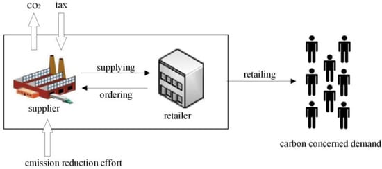
Figure 3.
The supply chain operation under tax policy.
Given the tax rate , we can rewrite the profit function (2) of the upstream supplier with the initial carbon emissions amount and emission-reduction efficiency as
As to the case without carbon policy and emission reduction investment, it is easy to obtain the retailer’s replenishment quantity as follows.
The difference of carbon emissions between the low-carbon supply chain and the traditional supply chain can be defined as , where represents the supplier’s carbon emissions in the low-carbon supply chain and represents the supplier’s carbon emissions in the traditional supply chain. Then, we can calculate and obtain as
The following proposition can be obtained.
Proposition 5.
(i) ; (ii) if and , then .
Proposition 5(i) indicates that the retailer always orders more in the low-carbon supply chain than in the traditional supply chain. The result in part (ii) of Proposition 5 is surprising: when is relatively high and is relatively low, the low-carbon supply chain under the optimal strategy will be no longer “low-carbon”. This demonstrates that for the pollution industries, the carbon tax policy may be invalid if environmental technology is not efficient enough to reduce carbon emissions.
4.2. Cap-and-Trade Policy
Under the cap-and-trade policy, the government allocates the supplier an initial carbon emission cap , and the supplier invests in green technology to reduce carbon emissions subject to the limited carbon quota. After the emissions reduction, the supplier will buy or sell emission permits at carbon price per unit of emission via a carbon trading market. The supplier’s trading willingness in the carbon market will depend on carbon price , that is, the supplier’s total cost after the transaction should be less than the pre-transaction one (see Figure 4).
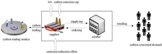
Figure 4.
The supply chain operation under cap-and-trade policy.
We can rewrite the profit function of the upstream supplier as
To further discuss the government allocates an emission cap based on the output of the enterprise, that is, the enterprise with higher output can get a larger cap and that with lower output can get a smaller cap. We can substitute for to make further analysis, where represents the carbon quota per unit of product allocated by the government.
Then, the supplier’s profit function can be changed equivalently to
Proposition 6.
The government allocates an emission cap according to the output brings higher supplier’s emission reduction level than according to the total cap, i.e., , and the difference between them is always positively influenced by both per-unit product allocation quota and carbon price .
Proof.
According Equations (21) and (22), similar to the proof for Proposition 5, we can solve the optimization problem faced by the supplier respectively, and when , the optimal effort level of emission reduction can be obtained as
Thus, it is easy to get .
This completes the proof. ☐
Proposition 6 shows that when the government allocates an emission cap based on the output, the supplier’s emission reduction level rises as increases and falls as decreases. That is, the supplier should develop different emission reduction strategies for different allocation policies of carbon quota set by the government in order to gain more market share.
4.3. The Analysis under the Joint Carbon Tax and Cap-and-Trade Policy
With a carbon tax policy, the firm’s carbon emissions reduction is affected by interactions between the tax rate and marginal costs of emission reduction. When the tax rate is lower while the marginal costs of emission reduction is higher, the effect of emissions reduction under the carbon tax policy will be worse, then a higher carbon price can be imposed by the market to achieve emission reduction. It is the same case with cap-and-trade policy. Based on the analysis, we investigate the joint carbon tax and cap-and-trade policy (see Figure 5).
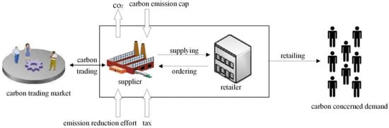
Figure 5.
The supply chain operation under the joint carbon tax and cap-and-trade policy.
Based on Equations (18) and (21), under the joint carbon tax and cap-and-trade policy, the optimal problem faced by the upstream supplier with policy parameters , , can be expressed as
Proposition 7.
Under the joint carbon tax and cap-and-trade policy, relationship between the carbon tax and the carbon price is complementary.
From the external policy standpoint, the carbon tax and carbon price are determined by the government regulation and carbon trading market respectively, therefore, the joint carbon tax and cap-and-trade policy is a mechanism of the government regulation and carbon trading market working together. As a result, relationship between the carbon tax and the carbon price is complementary, that is the lower the carbon price decided by the market is, the higher the tax rate imposed by the government is. With the rise of carbon price, intervention from the government experiences a gradual decline; similarly, with a relaxed tax rate, the carbon trading market will play a much larger role in reducing emissions.
5. Numerical Analysis
In this section, we present numerical analysis to graphically demonstrate the influence of emission reduction investment coefficient , consumer’s low-carbon preference , supplier’s overconfidence factor , and retailer’s overconfidence factor on managerial decisions and performance. Furthermore, we also provide numerical comparisons among three carbon policies under the supplier’s biased cognition. According to the model descriptions and assumptions in Section 2, we know that supplier’s overconfidence factor and retailer’s overconfidence factor satisfy and , respectively. Referring to literature [35,39], we specify that , , , , , , , , , , and .
5.1. The Optimal Emission Reduction Level, Replenishment Quantities, and Supply Chain Carbon Emissions
As can be seen from Figure 6 and Figure 7, under an overconfident supplier–rational retailer decentralized scenario, the supplier’s emission reduction level increases with both his overconfidence factor and consumer’s low-carbon preference , and decreases with emission reduction investment coefficient . Furthermore, Figure 8 shows the impact of the supplier’s overconfidence factor on his carbon emission reduction level; Figure 9 and Figure 10 respectively show under situation and under situation, how the supplier’s overconfidence factor and retailer’s overconfidence factor affect retailer’s replenishment quantity, here the parameters assignment are given as , , , under situation and , , , under situation; Figure 11, Figure 12 and Figure 13 show the impact of consumer’s low-carbon preference on the difference of carbon emissions . Meanwhile, is set to 0.4 in Figure 8, Figure 9 and Figure 10, is set to 0.6 in Figure 12, and is fixed to 1.5 in Figure 12 and Figure 13.
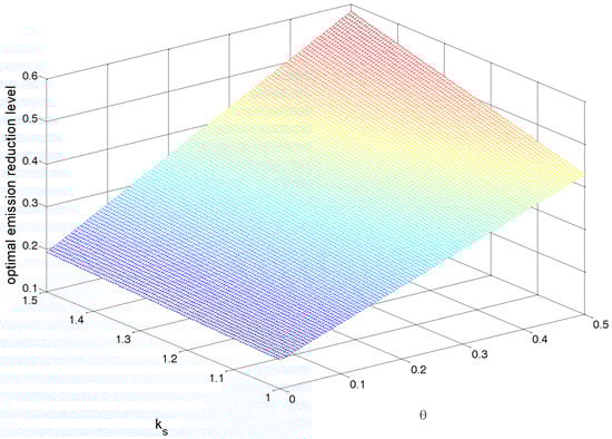
Figure 6.
Impacts of and on emission reduction level.
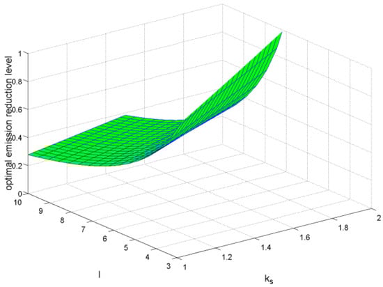
Figure 7.
Impacts of and on emission reduction level.
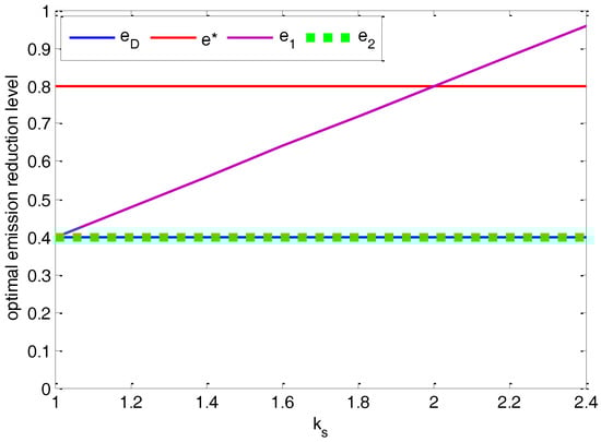
Figure 8.
Impacts of on emission reduction level.
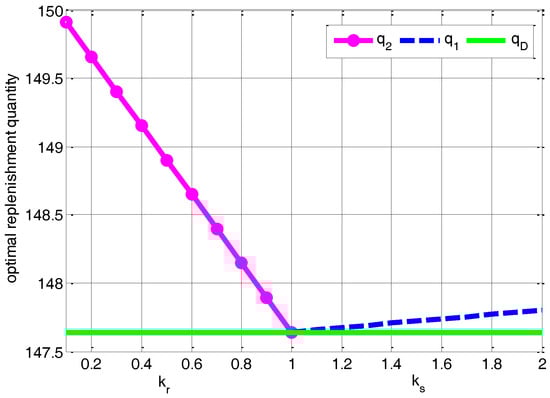
Figure 9.
Impacts of and on replenishment quantity under situation.
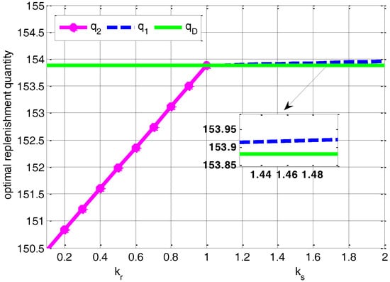
Figure 10.
Impacts of and on replenishment quantity under situation.
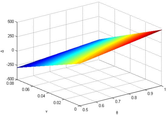
Figure 11.
Impacts of and on the difference of carbon emissions .
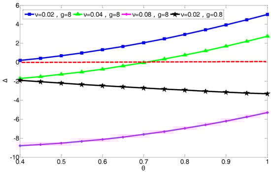
Figure 12.
Impacts of on the difference of carbon emissions .
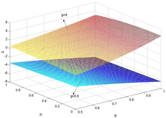
Figure 13.
Impacts of and on the difference of carbon emissions .
From Figure 8, we can see that if and , which shows that the supplier’s overconfidence mitigates double marginalization, if and , and if and , then the supplier’s emission reduction level exceeds the optimal one of the centralized system. Figure 8 also shows that , which illustrates that in a rational supplier–overconfident retailer decentralized scenario, the retailer’s overconfidence factor has no effect on the supplier’s emission reduction level.
Figure 9 exhibits that when , the increasing of retailer’s overconfidence factor results in the falling of his replenishment quantity under decentralized decision with a rational supplier–overconfident retailer and ; Figure 10 exhibits that when , the retailer’s replenishment quantity rises as increases and . In both cases, as the increases, the retailer will get the replenishment closer to the expected demand in response to the risk from underestimating of demand fluctuation. Incorporating Figure 9 and Figure 10, no matter what the critical fractile is, the retailer’s replenishment quantity see a constant rise with under decentralized decision with an overconfident supplier–rational retailer and .
Figure 11 reflects the relationship of carbon emissions between the low-carbon supply chain and the traditional supply chain. As can be seen from Figure 11, the difference of carbon emissions increases with consumer’s low-carbon preference and decreases with the emission-reduction efficiency .
In Figure 12, we set four cases to discuss the difference of carbon emissions . As is shown, when the emission-reduction efficiency is high (, ), carbon emissions of the low-carbon supply chain are less than those of the traditional supply chain; similarly, when is moderate (, ) and consumer’s low-carbon preference is low, carbon emissions of the low-carbon supply chain are also less than those of the traditional supply chain, but carbon emissions of the low-carbon supply chain increase in , and even surpass those of the traditional supply chain when increases to a certain high level, which makes the low-carbon supply chain no longer “low-carbon”; when is low (, ), carbon emissions of the low-carbon supply chain are more than those of the traditional supply chain. These results are consistent with Proposition 5. Interestingly, comparing , and , , we find that the values of initial carbon emissions amount decide on the correlation between the difference of carbon emissions and consumer’s low-carbon preference . As shown in Figure 13, our further analysis illustrates this issue.
From Figure 13, we can find that when , the difference of carbon emissions decreases in consumer’s low-carbon preference and carbon tax ; on the contrary, when , increases in and . The above results mean that for the clean industry, driven doubly by carbon tax and consumer’s low-carbon preference, the supplier in low-carbon supply chain would like to enhance emission reduction by technological innovation, and it is easy to reduce emissions; in turn, this implies that for the dirty industry, such a drive is counter-productive, and the reason might be that the cost of emission reduction by technological innovation is far more than carbon tax, and it is hard to reduce emissions. Meanwhile, if there are no effective substitute products, then the supplier would like to produce more to obtain profit, resulting in the rising of carbon emissions in low-carbon supply chain. Due to the symmetry of models, we can obtain the same results on cap-and-trade policy and the joint carbon tax and cap-and-trade policy. In summary, the government (the carbon trading market) should tighten the carbon constraint for the clean industry and relax the carbon constraint for the dirty industry.
5.2. Profitability Analysis
Figure 14 shows in the supplier overconfident case, the rising of supplier’s overconfidence factor results in the decreasing of the supplier’s profit and increasing of the retailer’s profit. Due to the profit decrement of the supplier being less than the profit increment of the retailer, the total supply chain profit is actually increased as increases. That is, the supplier’s overconfidence enhances the retailer's profit as well as the total supply chain at the cost of dropping his own profit.
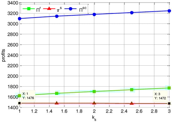
Figure 14.
Impacts of on profits.
In Figure 15, the plane () divides the curved surface into two parts. Let , , and , then when , the critical fractile is just equal to 0.5. When (i.e., the lower part of curved surface), the supplier’s profit increases in , but when (i.e., the upper part of curved surface), the supplier’s profit decreases in , which is in accordance with Proposition 4.
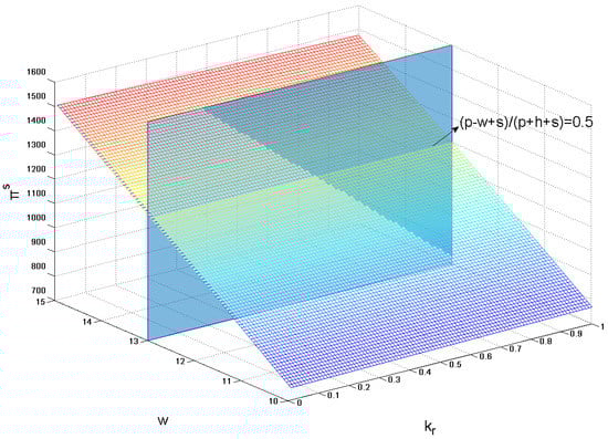
Figure 15.
Impacts of and on the supplier’s profit.
5.3. A Comparative Analysis of the Three Emission Policies
Figure 16A,B are used to compare the effect of emissions reduction in the supply chain under each carbon policy. We can see that all three policies are effective in reducing emissions, and the joint carbon tax and cap-and-trade policy results in lower carbon emissions than the tax and cap-and-trade do respectively; from the perspective of emission-reduction efficiency, the data cursors in Figure 16A,B demonstrate that the emission-reduction efficiency of the joint carbon tax and cap-and-trade policy is respectively more than that of the tax and of the cap-and-trade; incorporating Figure 16A,B, in case of parameters selections consistent with each other, the cap-and-trade could help firms to reduce more emissions than the tax, which implies that cap-and-trade policy is superior to tax policy under the same conditions. Figure 16A,B indicate respectively that carbon emissions in the supply chain remain high when the tax rate (carbon price ) is relatively low, and therefore it is necessary to supplement a cap-and-trade (a tax) that is lower carbon tax (carbon price ) to facilitate the market adjustment (the government intervention) to reduce the carbon emissions.
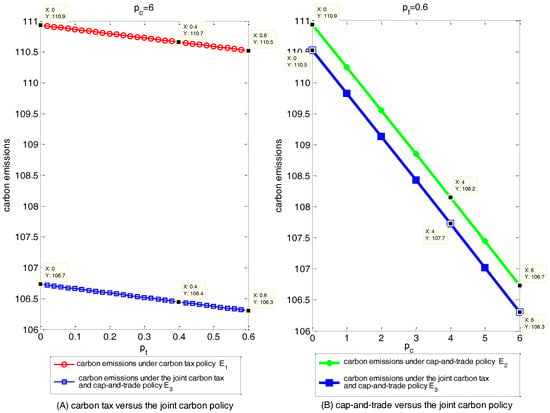
Figure 16.
The comparison of carbon emissions under different carbon policies.
Figure 17 reflects the complementary relationship between carbon tax and carbon price under the joint carbon tax and cap-and-trade policy. A certain carbon tax corresponds to a carbon price , and the corresponding carbon price decreases as the tax rate rises. That is when the government relaxes carbon tax policy, the carbon trading market will play a much larger role in reducing emissions, while, when the government tightens carbon tax policy, the role of the carbon trading market will experience a gradual decline.

Figure 17.
Carbon tax versus carbon price .
6. Conclusions
The paper develops models and game-theoretically analyzes low-carbon operations under four different scenarios (integrated SC, decentralized SC, decentralized SC with an overconfident supplier, and decentralized SC with an overconfident retailer). We characterize respectively supplier’s overconfidence and retailer’s overconfidence, and examine how overconfidence and consumer’s low-carbon preference impact the performances of each SC player and the whole SC.
The research makes several key contributions. First, unlike previous studies, we prove that the supplier’s overconfidence can mitigate double marginalization but hurt self-profit, while the retailer’s overconfidence can be an irrelevant factor for self-profit. Second, our research findings have some interesting managerial insights. For instance, the retailer aiming at short-term trading should actively seek an overconfident supplier, while the supplier should actively seek a rational retailer for whom the critical fractile is more than 0.5, whereas for an overconfident retailer, the critical fractile is less than or equal to 0.5. Finally, our simulation results also provide important policy implications. For example, cap-and-trade policy is superior to tax policy under the same conditions; the joint carbon tax and cap-and-trade policy works best for emission-reduction amount or emission-reduction efficiency; the government (the carbon trading market) should tighten the carbon constraint for the clean industry and relax the carbon constraint for the dirty industry.
Further studies may consider the wholesale price as an endogenous variable, which changes with emission reduction level of the supplier, and concentrate on the case that the supplier’s and the retailer’s overconfidence are asymmetric.
Acknowledgments
This work was supported by the National Natural Science Foundation of China (No. 71572031), Philosophy and Social Science Fund of Liaoning, China (No. L16AZY032).
Author Contributions
Shoufeng Ji and Dan Zhao contributed in developing the ideas of this research. Shoufeng Ji, Dan Zhao, and Xiaoshuai Peng performed this research. All the authors involved in preparing this manuscript.
Conflicts of Interest
The authors declare no conflict of interest.
Nomenclature
The following notations are used in this paper.
| Parameters: | |||
| market demand | supplier’s overconfidence factor | ||
| market potential | retailer’s overconfidence factor | ||
| sensitivity coefficient of demand on retail price | marginal production cost of the supplier | ||
| consumer’s low-carbon preference | emission reduction investment coefficient | ||
| random variable of the market demand | unit holding cost from retailer | ||
| product retail price | unit shortage cost from retailer | ||
| product wholesale price | |||
| Decision variables: | |||
| the level of emission reduction effort devoted by the supplier | retailer’s replenishment quantity | ||
Appendix A
Proof of Proposition 2.
(i) From Equation (13), we have by differentiating with respect to , thus incorporating the assumption , we get , i.e., the retailer’s replenishment quantity rises as supplier’s overconfidence factor increases. Similarly, according to Equations (8) and (13), we have , and incorporating the assumption and , we can obtain .
(ii) Equation transformed from equation can be expressed as , where . According to the properties of the CDF, we know that when , so and the retailer’s replenishment quantity rises as his overconfidence factor falls. Similarly, when , so and the retailer’s replenishment quantity falls as decreases. From Equations (8) and (17), we obtain , where , , and . According to the properties of the CDF, we know that when , so , and when , so .
Proof of Proposition 3.
Substituting Equations (12) and (13) into Equation (2), we can obtain . The first derivation of regarding is , so the supplier’s profit decreases with his overconfidence factor ; substituting Equations (12) and (13) into Equation (1), we obtain , where . The first derivation of regarding is , the retailer’s profit increases with supplier’s overconfidence factor .
Proof of Proposition 5.
Combining Equation (18) with Equation (11) yields , we further derive and . It is obvious that when , and set , we can obtain the optimal emission reduction efforts of the supplier as .
However, Equation (11) is a mathematical projection under tax policy when the supplier is overconfident, and the actual response function of the retailer should be expressed as , and incorporating , we can obtain that the optimal replenishment quantity of the retailer is .
This completes the proof.
References
- GBD 2013 Mortality and Causes of Death Collaborators. Global, regional, and national age-sex specific all-cause and cause-specific mortality for 240 causes of death, 1990–2013: A systematic analysis for the global burden of disease study 2013. Lancet 2015, 385, 117–171. [Google Scholar]
- Liu, Z.; Anderson, T.D.; Cruz, J.M. Consumer environmental awareness and competition in two-stage supply chains. Eur. J. Oper. Res. 2012, 218, 602–613. [Google Scholar] [CrossRef]
- Cachon, G.P. Retail store density and the cost of greenhouse gas emissions. Manag. Sci. 2014, 60, 1907–1925. [Google Scholar] [CrossRef]
- Hoen, K.M.; Tan, T.; Fransoo, J.C.; van Houtum, G.-J. Switching transport modes to meet voluntary carbon emission targets. Transp. Sci. 2013, 48, 592–608. [Google Scholar] [CrossRef]
- Hua, G.; Cheng, T.; Wang, S. Managing carbon footprints in inventory management. Int. J. Prod. Econ. 2011, 132, 178–185. [Google Scholar] [CrossRef]
- Bouchery, Y.; Ghaffari, A.; Jemai, Z.; Dallery, Y. Including sustainability criteria into inventory models. Eur. J. Oper. Res. 2012, 222, 229–240. [Google Scholar] [CrossRef]
- Drake, D.F.; Kleindorfer, P.R.; Van Wassenhove, L.N. Technology choice and capacity portfolios under emissions regulation. Prod. Oper. Manag. 2016, 25, 1006–1025. [Google Scholar] [CrossRef]
- Du, S.; Hu, L.; Wang, L. Low-carbon supply policies and supply chain performance with carbon concerned demand. Ann. Oper. Res. 2017, 255, 569–590. [Google Scholar] [CrossRef]
- Plambeck, E.L. Reducing greenhouse gas emissions through operations and supply chain management. Energy Econ. 2012, 34, 64–74. [Google Scholar] [CrossRef]
- Uebelhoer, K.; Guder, J.; Holst, J.C.; Heftrich, B. Greenhouse gas management along the supply chain at siemens. In Proceedings of the 6th International Conference on Life Cycle Management, Gothenburg, Sweden, 25–28 August 2013. [Google Scholar]
- Dong, C.; Shen, B.; Chow, P.S.; Yang, L.; Chi, T.N. Sustainability investment under cap-and-trade regulation. Ann. Oper. Res. 2016, 240, 509–531. [Google Scholar] [CrossRef]
- Xu, J.; Chen, Y.; Bai, Q. A two-echelon sustainable supply chain coordination under cap-and-trade regulation. J. Clean. Prod. 2016, 135, 42–56. [Google Scholar] [CrossRef]
- Benjaafar, S.; Li, Y.; Daskin, M. Carbon footprint and the management of supply chains: Insights from simple models. IEEE Trans. Autom. Sci. Eng. 2013, 10, 99–116. [Google Scholar] [CrossRef]
- Chen, X.; Benjaafar, S.; Elomri, A. The carbon-constrained eoq. Oper. Res. Lett. 2013, 41, 172–179. [Google Scholar] [CrossRef]
- Toptal, A.; Özlü, H.; Konur, D. Joint decisions on inventory replenishment and emission reduction investment under different emission regulations. Int. J. Prod. Res. 2014, 52, 243–269. [Google Scholar] [CrossRef]
- Żuchowski, W. Division of environmentally sustainable solutions in warehouse management and example methods of their evaluation. LogForum 2015, 11, 171–182. [Google Scholar] [CrossRef]
- Chen, X.; Wang, X.; Kumar, V.; Kumar, N. Low carbon warehouse management under cap-and-trade policy. J. Clean. Prod. 2016, 139, 894–904. [Google Scholar] [CrossRef]
- Atasu, A.; Sarvary, M.; Wassenhove, L.N.V. Remanufacturing as a marketing strategy. Manag. Sci. 2008, 54, 1731–1746. [Google Scholar] [CrossRef]
- Chitra, K. In search of the green consumers: A perceptual study. J. Serv. Res. 2007, 7, 173–191. [Google Scholar]
- Geyer, R.; Van Wassenhove, L.N.; Atasu, A. The economics of remanufacturing under limited component durability and finite product life cycles. Manag. Sci. 2007, 53, 88–100. [Google Scholar] [CrossRef]
- Savaskan, R.C.; Bhattacharya, S.; Van Wassenhove, L.N. Closed-loop supply chain models with product remanufacturing. Manag. Sci. 2004, 50, 239–252. [Google Scholar] [CrossRef]
- Savaskan, R.C.; Van Wassenhove, L.N. Reverse channel design: The case of competing retailers. Manag. Sci. 2006, 52, 1–14. [Google Scholar] [CrossRef]
- Li, X.; Li, Y. Chain-to-chain competition on product sustainability. J. Clean. Prod. 2016, 112, 2058–2065. [Google Scholar] [CrossRef]
- Zhang, L.; Wang, J.; You, J. Consumer environmental awareness and channel coordination with two substitutable products. Eur. J. Oper. Res. 2015, 241, 63–73. [Google Scholar] [CrossRef]
- Zhou, Y.; Bao, M.; Chen, X.; Xu, X. Co-op advertising and emission reduction cost sharing contracts and coordination in low-carbon supply chain based on fairness concerns. J. Clean. Prod. 2016, 133, 402–413. [Google Scholar] [CrossRef]
- Swami, S.; Shah, J. Channel coordination in green supply chain management. J. Oper. Res. Soc. 2013, 64, 336–351. [Google Scholar] [CrossRef]
- Du, S.; Zhu, J.; Jiao, H.; Ye, W. Game-theoretical analysis for supply chain with consumer preference to low carbon. Int. J. Prod. Res. 2015, 53, 3753–3768. [Google Scholar] [CrossRef]
- Moore, D.A.; Healy, P.J. The trouble with overconfidence. Psychol. Rev. 2008, 115, 502–517. [Google Scholar] [CrossRef] [PubMed]
- Bostian, A.J.A.; Holt, C.A.; Smith, A.M. Newsvendor “pull-to-center” effect: Adaptive learning in a laboratory experiment. Manuf. Serv. Oper. Manag. 2008, 10, 590–608. [Google Scholar] [CrossRef]
- Van den Steen, E. Overconfidence by bayesian-rational agents. Manag. Sci. 2011, 57, 884–896. [Google Scholar] [CrossRef]
- Hambrick, D.C. Upper echelons theory: An update. Acad. Manag. Rev. 2007, 32, 334–343. [Google Scholar] [CrossRef]
- Ancarani, A.; Mauro, C.D.; D’Urso, D. Measuring overconfidence in inventory management decisions. J. Purch. Supply Manag. 2016, 22, 171–180. [Google Scholar] [CrossRef]
- Bendoly, E.; Croson, R.; Goncalves, P.; Schultz, K. Bodies of knowledge for research in behavioral operations. Prod. Oper. Manag. 2010, 19, 434–452. [Google Scholar] [CrossRef]
- Croson, D.; Croson, R.; Ren, Y. How to Manage an Overconfident Newsvendor; Working Paper; Cox School of Business, Southern Methodist University: Dallas, TX, USA, 2008. [Google Scholar]
- Lu, X.; Shang, J.; Wu, S.-Y.; Hegde, G.G.; Vargas, L.; Zhao, D. Impacts of supplier hubris on inventory decisions and green manufacturing endeavors. Eur. J. Oper. Res. 2015, 245, 121–132. [Google Scholar] [CrossRef]
- Ren, Y.; Croson, R. Overconfidence in newsvendor orders: An experimental study. Manag. Sci. 2013, 59, 2502–2517. [Google Scholar] [CrossRef]
- Li, M.; Petruzzi, N.C.; Zhang, J. Overconfident competing newsvendors. Manag. Sci. 2016, 63, 2637–2646. [Google Scholar] [CrossRef]
- Yue, J.; Austin, J.; Wang, M.-C.; Huang, Z. Coordination of cooperative advertising in a two-level supply chain when manufacturer offers discount. Eur. J. Oper. Res. 2006, 168, 65–85. [Google Scholar] [CrossRef]
- Wang, Q.; Zhao, D.; He, L. Contracting emission reduction for supply chains considering market low-carbon preference. J. Clean. Prod. 2016, 120, 72–84. [Google Scholar] [CrossRef]
- Petruzzi, N.C.; Dada, M. Pricing and the newsvendor problem: A review with extensions. Oper. Res. 1999, 47, 183–194. [Google Scholar] [CrossRef]
© 2018 by the authors. Licensee MDPI, Basel, Switzerland. This article is an open access article distributed under the terms and conditions of the Creative Commons Attribution (CC BY) license (http://creativecommons.org/licenses/by/4.0/).