Environmental Fiscal Reform and the Double Dividend: Evidence from a Dynamic General Equilibrium Model


1
Department of Economics, Harvard University, Cambridge, MA 02138, USA
2
ENT Environment and Management, Sant Joan, 39, 1, Vilanova i la Geltrú, 08800 Barcelona, Spain
3
Harvard China Project on Energy, Economy and Environment, Harvard University, Cambridge, MA 02138, USA
*
Author to whom correspondence should be addressed.
Sustainability 2018, 10(2), 501; https://doi.org/10.3390/su10020501
Submission received: 12 December 2017
/
Revised: 29 January 2018
/
Accepted: 2 February 2018
/
Published: 13 February 2018
(This article belongs to the Section Economic and Business Aspects of Sustainability)
Abstract
:An environmental fiscal reform (EFR) represents a transition of a taxation system toward one based in environmental taxation, rather than on taxation of capital, labor, or consumption. It differs from an environmental tax reform (ETR) in that an EFR also includes a reform of subsidies which counteract environmental policy. This research details different ways in which an EFR is not only possible but also a good option that provides economic and environmental benefits. We have developed a detailed dynamic CGE model examining 101 industries and commodities in Spain, with an energy and an environmental extension comprising 31 pollutant emissions, in order to simulate the economic and environmental effects of an EFR. The reform focuses on 39 industries related to the energy, water, transport and waste sectors. We simulate an increase in taxes and a reduction on subsidies for these industries and at the same time we use new revenues to reduce labor, capital and consumption taxes. All revenue recycling options provide both economic and environmental benefits, suggesting that the “double dividend” hypothesis can be achieved. After three to four years after implementing an EFR, GDP is higher than the base case, hydrocarbons consumption declines and all analyzed pollutants show a reduction.
1. Introduction
There is a growing consensus in the European Union that environmental taxes are a promising policy for reducing environmental impacts and also as a way to increase public revenues and reduce fiscal pressure [1]. Revenues from environmental taxes in Spain are the lowest in the EU-27, accounting for 1.57% of gross domestic product (GDP), far below the EU average, which was 2.40% in 2012. As is the case in most of the EU’s member states, environmental taxation in Spain is mostly focused on energy (1.3% of GDP) [2]. In the recent years, the European Commission has recommended that Spain increase its environmental taxes in order to converge with those of other Member States and to increase its public revenues [3]. The “Europe 2020” strategy calls for implementing policies that shift part of the tax base to environmentally damaging activities; this strategy is a vital part of an overall policy package that aims to tackle these multiple challenges [4].
The theoretical basis of environmental taxes has been well documented in early discussions of Baumol, Baumol and Oates [5,6]; such taxes create incentives to change behaviors toward sustainability targets in a Pigouvian sense [7]. The objective of an environmental tax is to reduce/internalize a negative externality such as pollution or natural resources exhaustion. The social benefits of a Pigouvian tax could outstrip its costs.
An environmental tax reform (ETR) consists in transitioning the national taxation system based on extant taxes on labor (personal income tax and social contributions), capital and consumption (VAT and other indirect taxes) to one based on consumption and production activities that generate environmental pressures, without affecting the overall government revenues coming from taxation. This shift could provide better signals to economic agents, leading to better functioning of markets. In a more general way, an environmental fiscal reform (EFR) also includes the elimination of environmentally harmful subsidies [1]. Some authors argue that this type of reform would reduce environmental impacts while at the same time improving the economy.
The “double dividend hypothesis” suggests that introducing environmental taxes and using the associated revenues to reduce other taxes not only reduces environmental problems but also has a positive impact on the economy, so long as the state maintains a constant level of total revenue and/or government expenditure [8,9,10,11]. However, the literature shows that there are uncertainties regarding the economic and environmental effects of such a reform in a specific region [12,13,14,15]. These studies also show that different schema for implementing an ETR or an EFR would lead to different results in terms of economic and environmental achievements.
Computable general equilibrium (CGE) models are the most comprehensive way to take into account the most relevant aspects of an economic system [16]. They allow researchers to assess the effect on different macroeconomic variables from external impacts or policies, such as changes to a taxation system. Some recent studies that have used CGE methods to model the effects of an ETR. Bye (2000), Ciaschini et al. (2012), Fernández et al. (2011), Holmlund and Kolm (2000), Jorgenson et al. (2013), Patuelli et al. (2005) and Wendner (2001) [17,18,19,20,21,22,23] all found that a carbon tax on the United States economy could achieve a double dividend by recycling revenues in capital taxes. A literature review on CGE modeling and the double dividend can be found in Freire-González [24] which draws two main conclusions: first, an environmental tax improves environmental conditions, which is the main objective of imposing such a tax; and second, the post-reform improvement of economic conditions remains uncertain. However, most simulations analyzed achieved a double dividend and literature shows that recycling government revenues to reduce other pre-existing taxes minimize costs. Bosquet [25] reviews the early literature on the use of simulations to analyze the double dividend hypothesis, finding some evidence of support in particular cases but also suggests potential improvements that this approach would benefit from. Also, Ekins and Speck [26] conducted a review of the subject, suggesting that in practice in the EU, many industries have circumvented the environmental taxes due to fears over competitiveness in the EU.
In the specific context of Spain, there are a number of extant studies that analyze the effects of environmental taxation and address their potential (e.g., [27,28,29,30]). Some studies use CGE models to assess the impact of environmental taxes, especially energy taxes, on the Spanish economy [31,32,33,34]. Few scholars have analyzed different forms of an ETR from a general equilibrium perspective [35,36,37].
In this research, we develop a dynamic CGE model that is highly disaggregated, encompassing 101 industries and commodities, to assess the economic and environmental effects of an EFR focused on the energy, water, transport and waste sectors in Spain. This is something that has never done before at this detail. We increase output taxes and reduce subsidies for 39 industries related to those sectors and use the government revenues generated to cut other pre-existing taxes, thus instituting a revenue-neutral reform. Specifically, we use these revenues to reduce value-added taxes along with taxes on capital and labor, testing the double dividend hypothesis for an EFR in Spain. Beyond the economic impacts of the reform, we also assess its effects on 31 different local and global pollutants and on the total use of coal, oil and gas. While a direct tax on pollutant emissions would create effective incentives, changing output taxes and subsidies is currently a common way to do an EFR in Spain and in Europe, even though there are many countries in the context of Europe, or the rest of the world that use pollutant or externality taxes (like a carbon tax). A description of the model follows in Section 2; Section 3 describes the data and the assumptions on exogenous variables; Section 4 describes the scenarios and the results of simulations and Section 5 lays out the main conclusions of the research.
2. The Energy-Environment-Economy Dynamic CGE Model
A dynamic CGE model for the Spanish economy is developed in this research. It is based on and has a structure similar to previous models developed by Dale Jorgenson and colleagues, previously used in Cao et al. (2009), Cao et al. (2013), Ho and Jorgenson (2007), Jorgenson et al. (2013) and Jorgenson and Wilcoxen (1993) [21,38,39,40,41], among others. A previous version of this model can be found in Freire-González and Ho [42]. The relevant features and adaptations are detailed in this section and in the technical Appendix A. The main characteristic of this model is that growth is driven by savings; thus, conceptually, it is a Solow growth based model. Savings come from three main sources: households, enterprises and the foreign sector. Households save a share of their income, enterprises retain part of their earnings and foreign sector invests through foreign investment. These savings finance the government deficit and are used for investment in domestic capital. Economic growth depends on population growth, capital accumulation and technical change or growth in total factor productivity.
As in many other CGE models, different agents are identified. They both receive and spend incomes and have other roles represented by the equations system shown in Appendix A. The four main agents represented in this system are:
- Households: Their main role is to supply labor, purchase goods and services and receive incomes from the labor they supply, from the capital and land they own, from the government and from the rest of the world. Households also pay taxes to government and save part of their total income.
- Government: Its main economic role is to collect and redistribute other agents’ incomes though taxes, subsidies and transfers. In our model, we categorize these taxes as tax on capital; tax on labor; property tax; tax on dividends; value-added tax (VAT) on products; special taxes on alcohol, tobacco, hydrocarbons, electricity and retail hydrocarbons; sales tax; other taxes on production; social security contributions; and import taxes (or tariffs). We also factor in other non-tax revenues from households and companies, along with production subsidies. The government also buys goods and services, invests and pays interests for government bonds. Government deficits are covered by domestic and foreign borrowing.
- Enterprises: Their role is mainly to produce commodities using intermediate and primary inputs purchased in the market; their revenue includes government output subsidies and other payments. They spend their earnings on dividends to households and taxes to government; they also save a share of their income by retaining part of the earnings. Regarding production, the model identifies 101 industries that produce 101 commodities, with high levels of detail in the electricity generation and waste treatment technology sectors.
The factors of production are capital, labor, land, energy and other intermediates. Production functions are specified as Cobb-Douglas technology functions with constant returns to scale, as output expands in proportion to inputs (There are no estimates of elasticities of substitution at this level of detail. Many models assume a fixed coefficient—Leontief—function for intermediate inputs, however, this is not consistent with data at the industry level; time series of input-output tables in many countries show substantial changes in most input coefficients.) Technical coefficients can change over time in two different ways: (1) there is technical progress, meaning that there is more output with the same inputs; and (2) there is biased technical change, i.e. changes in input demands unrelated to prices. The capital input for each industry is rented from a total capital stock that changes over time; it increases with new investments and decreases with depreciation. Labor is assumed to be mobile across sectors and the labor supply depends on the level of unemployment. The land factor has been designated for the agriculture, forestry and fishing industries and its supply is fixed exogenously.
- Rest of world: Its main role it to purchase exports, sell imports and provide foreign investment. It also receives and pays incomes from other agents. Imports and domestic output follow Armington’s assumption [43], to be combined through constant elasticity of substitution (CES) functions, producing a composite commodity supply.
The CGE model includes a submodel describing energy use and the emissions of 31 pollutants. Specifically, consumption of coal, oil, natural gas and electricity are identified. These energy coefficients (described in Appendix A) were estimated using data from the International Energy Agency (IEA) on total energy consumption and input-output tables for Spain; in this way, we were able to estimate total energy consumption over time and under the different policies simulated. As there is no available data at the industry level on the use of hydrocarbons for the 101 sectors considered, an average coefficient has been used. This allows for an estimation of overall energy use.
To obtain CO2 emissions from energy use, we linked them using data from IEA (2016) [44] on CO2 emissions from fuel combustion of coal, oil and natural gas. Along with CO2, we have included 31 additional pollutants in the environmental module—some related to global warming, others more related to health risks. Coefficients for each pollutant and industry have been calculated from emissions data from Exiobase datasets for each industry.
3. Data
Implementing the model described above requires a massive amount of data. In this section, we describe the data we used to feed the model. A combination of economic and environmental data translated into the various parameters and variables needed to first calibrate the model and then to run simulations.
The main source of the economic data is a social accounting matrix (SAM) for the Spanish economy. This is a square matrix that provides information on the different flows of payments among the various elements of the economic system described: commodities, industries, capital, labor, land, households, enterprises, government, taxes and tariffs, investments, savings and the exterior sector. We have built a SAM that differentiates between commodities and industries, employing both supply and use tables. Supply and use tables have been developed using information from the National Statistics Institute of Spain (INE) and Exiobase [45,46]. Exiobase provides an input-output framework for 2007 that includes environmental information at a detailed industry level, disaggregated for 163 industries and 200 commodities. With the INE tables as a starting point, we developed new supply and use matrices by breaking down electricity and waste treatment industries using information from the Exiobase tables. In this way, we were able to complete the SAM while avoiding heterogeneity problems with other sources of information. The other information needed to complete the SAM comes from the INE and the Spanish government. After adjustments (Some industries have been aggregated to correspond with similar industries or commodities, thus reducing the number of very small or irrelevant industries from the analysis.), the resulting matrix encompasses 101 industries and 101 commodities, with high detail in the areas of electricity generation technologies (coal, gas, nuclear, hydro, wind, petroleum, biomass, solar, wave, geothermal and other) and waste treatment technologies (incineration, biogasification, composting and landfill). INE and Exiobase tables also provide other information needed to feed the SAM, such as final demand components, imports and data on taxes, compensation of employees, employment and operating surplus. The EU KLEMS project on growth and productivity provided data on the stock of capital and depreciation rates by industry [47]. The SAM also includes details on different forms of industry taxation, including VAT, sales taxes, other taxes on products, tariffs and VAT imports.
The matrix also includes economic information on income flows between agents. Figures for government accounts, including social security and tax accounts, have been obtained from the General Intervention Board of the State Administration (IGAE). Figures for foreign sector accounts have been obtained from the INE; they contain a detail on the balance of payments. Enterprise accounts have been obtained from the Bank of Spain and include details on the annual accounts of firms.
Besides the economic information, the model is fed with energy and environmental data. Figures for the consumption of coal, oil and natural gas and the resultant CO2 emissions, have been obtained from the IEA [44]. The information on the emissions of the other pollutants modeled have been obtained from the Exiobase dataset.
A summary of the described SAM for the Spanish economy for 2007 is shown in Table 1. We have four different agents represented in the SAM: households, government, enterprises and foreign sector. There are 15 big columns and rows, representing the different aspects we detail in our system. The detailed SAM contains a total of 119 columns and rows, including all industries, all commodities, a detail of different taxes, etc. Columns represent the payments and rows represent the receipts of incomes. In this way, all transactions between economic sectors and agents are represented as a square matrix. For instance, in the Households column we can see expenditures of €604,429 million in goods and services; the Government column shows total transfers of €155,808 million from public institutions to households. Cells should not be read literally, as in some cases we have considered net values, implying payments less charges. For instance, the Enterprise column considers payments to government (mainly from corporate income tax) minus transfers from the government to enterprises, yielding a net payment from enterprises to government of €89,388 million.
Some of the variables of the model are set exogenously. Most of them have been kept constant during the entire 30-year period assessed in this research, given the uncertainty regarding their evolution and the purpose of this research. However, different projections can be assumed depending on the expected evolution or the objective of the analysis. The variables that has been kept constant are government deficit share of GDP, interest paid by government, government payments to the rest of the world, net transfers from the rest of the world to households and dividend rate. The parameters of household consumption and investments have also kept constant. Savings rate and technical input-output coefficients are assumed to be unchanged during the period of analysis. Projections on population for the next years have been obtained from the INE. The sectoral labor force figure is based on working-age population data from Exiobase and has been assumed to increase at a same rate as the population. Growth of total factor productivity (TFP) is calibrated to produce an annual GDP growth rate of around 2% per year and the current account deficit is projected to decline.
4. Scenarios and Results
This section describes the policy scenarios simulated with the model and the results obtained in terms of economic and environmental impacts. The literature discusses the best option for recycling the revenues generated by environmental taxes. Most studies suggest that recycling them through lowering distortionary taxes is more efficient than returning them via lump-sum transfers to households or other economic agents [14,21,48,49,50,51].
The EFR we simulate is predicated on adding/increasing a tax on 39 different industry outputs while reducing/eliminating subsidies in those same industries. Specifically, the new tax represents a 20% of total output; subsidies are correspondingly reduced by 20% of their total output (Total output is variable QI, detailed in Equation (A3) from the Appendix A.1). The new tax is equivalent to an ad valorem tax of 20%. Levied industries are related to energy sectors; water supply; sales of motor vehicles and water and air transport; and waste treatment activities:
- Energy industry reforms are expected to increase the price of energy, thus reducing overall demand and consequently the emission of several pollutants. Particularly, they are expected to have a specific impact on GHG emissions. In our model, there are 16 industries in this category: coal and lignite peat; extraction of crude petroleum and services related to crude oil extraction; extraction of natural gas and services related to natural gas extraction, excluding surveying and mining of uranium and thorium ores; coke, refinement of petroleum and nuclear fuel; electricity by coal; electricity by gas; electricity by nuclear; electricity by hydro; electricity by wind; electricity by petroleum and other oil derivatives, electricity by biomass and waste, electricity by solar photovoltaic; electricity by solar thermal; electricity (other); transmission services of electricity; distribution and trade services of electricity; and production and distribution of natural gas.
- Water supply industry fiscal reform is expected to increase the price of water and thereby reduce its consumption. This reduction is not reflected in air pollutants modeled in this research but is consistent with an EFR that aims to reduce environmental loads. Given the constraints of the model, we tax the overall sector; in practice, however, the reform should be implemented as a progressive tax. The specific industry affected is: “Collected and purified water, distribution services of water”.
- Fiscal reform of transport industries is expected to have an effect similar to that of taxation of water, increasing the price of levied transport and reducing its consumption. We have simulated affectation on three transport industries, with different types of effects, some related to the production of transport units and some to their use: (i) “Sale of motor vehicles” would reduce purchases of motor vehicles and thus the externalities associated with their production; (ii) “Retail trade services of motor fuel” would reduce the use of motor vehicles and therefore the externalities associated with their use; (iii) “Air transport services” would reduce the use of air transportation.
- Waste-treatment industry reform aims to increase the costs and market prices of waste treatment and thereby to reduce waste generation. Consequently, pollutants associated with waste treatment would drop. There are 19 industries in this category: food waste for treatment—incineration; paper waste for treatment—incineration; plastic waste for treatment—incineration; inert/metal waste for treatment—incineration; textiles waste for treatment—incineration; wood waste for treatment—incineration; oil/hazardous waste for treatment—incineration; food waste for treatment—biogasification and land application; paper waste for treatment—biogasification and land application; sewage sludge for treatment—biogasification and land application; food waste for treatment—composting and land application; food waste for treatment—wastewater treatment; other waste for treatment—wastewater treatment; food waste for treatment—landfill; paper for treatment—landfill; plastic waste for treatment—landfill; inert/metal/hazardous waste for treatment—landfill; textiles waste for treatment—landfill; and wood waste for treatment—landfill.
Additionally, we use the increase in government revenues (from the new environmental taxes) and the reduction in government spending (from reduced subsidies) from these fiscal changes to reduce other pre-existing taxes. We set four different scenarios related to revenue recycling: a reduction of taxes on capital; a reduction of taxes on labor; a reduction of value-added taxes; and a scenario where revenues are not recycled, so there is more government spending. If the government’s deficit is kept constant, government spending must be the same as in the base case. We introduce an additional endogenous variable into the equations system, to scale the tax rates:
where is the tax rate for the tax (in our case, the tax on capital, the tax on labor, or the VAT) and industry , under the EFR and the 0 subscript denotes base case values. We also incorporate an additional restriction into the model to keep government expenditures neutral:
where is the quantity of aggregate government purchases (see Equation (A29) in the Appendix A.3). This variable is endogenous in the base case and exogenous in the policy scenario. In this policy scenario, the tax scale variable () and tax rates of modified pre-existing taxes become endogenous.
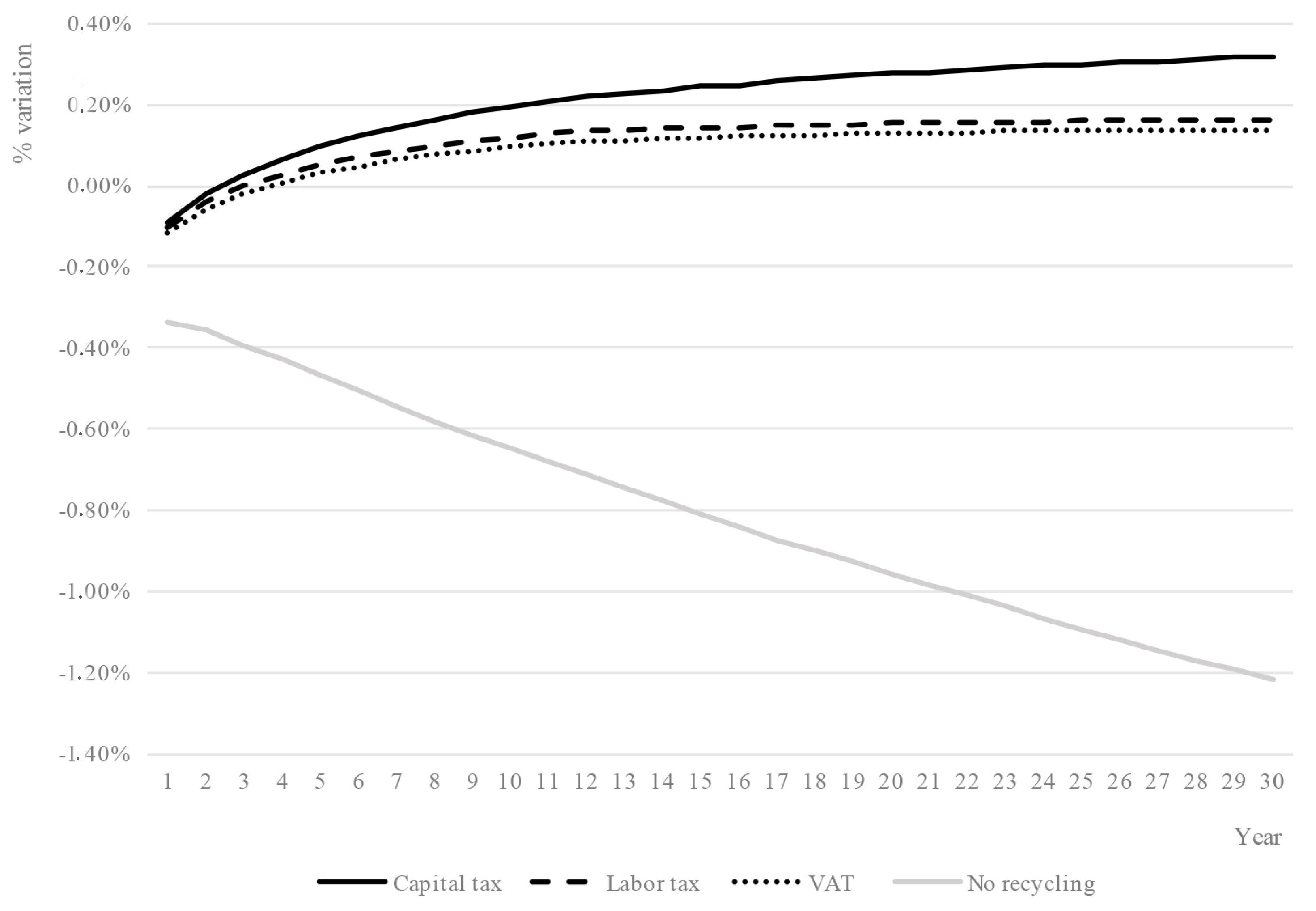
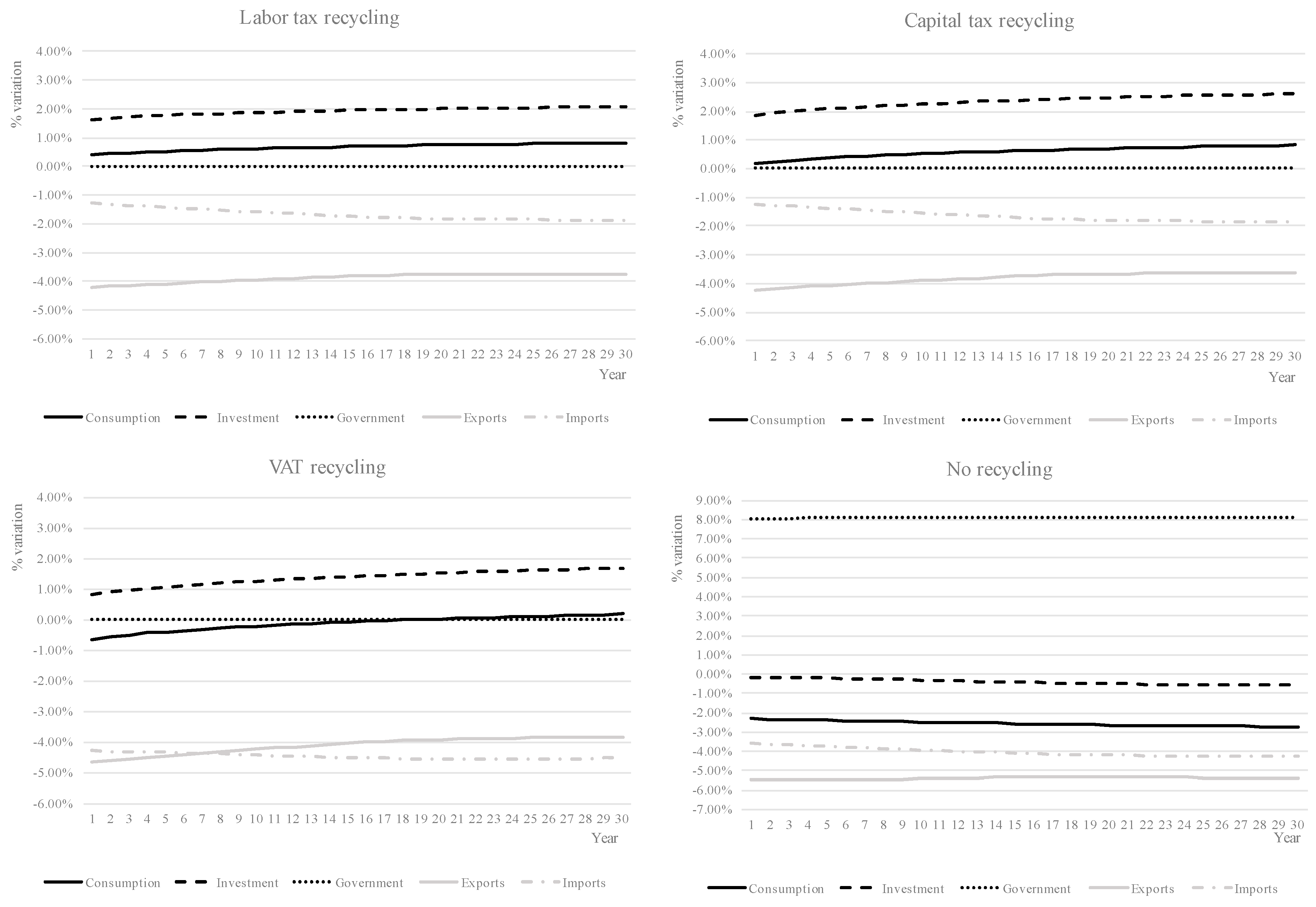
The first simulation conducted—the base case scenario—was performed using the initial information included in the SAM, using the actual tax rates to obtain a base-case growth path. Then, we ran the model with the EFR—adding or modifying taxes and subsidies on targeted industries in order to compare the obtained results with the base case. The main macroeconomic results for the described scenarios are presented in Figure 1 and Figure 2. Figure 1 shows the evolution of the percentage variation of GDP of an EFR under the different recycling scenarios described. Figure 2 shows the percentage variation of different components of GDP under the different scenarios—specifically, consumption, investment, public spending, exports and imports—projected for 30 years.
In all revenue-recycling scenarios, we observe a fall in GDP in the first few years of the EFR but higher investment eventually led to a higher GDP than in the base case. The scenario with no recycling of revenues, by contrast, shows a sustained decrease in GDP when compared to the base case. In pure efficiency terms, cutting capital taxes is the option that generates the highest economic benefit in the mid- and long-term. Different recycling scenarios lead to evolution of GDP components along different paths, as shown in Figure 2. Labor and capital tax recycling produce a greater increase in consumption than in other components, while capital tax recycling triggers the greatest improvement in investment. This shift towards investment comes from improved terms of trade that reduces exports in the 3 recycling scenarios. In the VAT cut case there is also a reduction in consumption in the first few years. We observe that in the scenario with no revenue recycling, only government purchases increase; the rest of the components decrease.
Analyzing industry-level results, we observe that as the new taxes rise, cost and prices increase and output falls; this is particularly pronounced in directly levied industries but also occurs in other related industries that buy inputs from them. This pattern is observed in all recycling scenarios, with small differences.
Regarding the energy consumption and the environmental consequences of an EFR, we observe an annual average reduction in coal consumption of 24.6%; an annual average reduction of 7% for oil consumption; and 36.9% for natural gas consumption. The differences among the scenarios are so small as to be insignificant, so a mean value is shown. Similarly, Table 2 shows the average annual percentage variation on emissions of 31 pollutants for the different projected scenarios.
All pollutants show a reduction in relation to the base case, as most of them are directly or indirectly related to the affected industries. Greenhouse gases or climate change related pollutants deserve special consideration here; they experience an important annual reduction with the EFR: CO2 drops by 14%; CH4 reduces 44.14%; N2O reduces 4.9% and HFC reduces 3.42%. There is also an important reduction in some pollutants that produce damaging health effects, such as SO2, which sees a 24.47% reduction; NOx, with a 16.3% reduction; and Se, with a 22.39% reduction. Thus, the tested EFR triggers an important reduction of pollutant emissions related to both climate change and health risks.
5. Conclusions
This article investigates the potential of an EFR to tackle climate change and health risks without disrupting the economic system. We develop a dynamic CGE model with an energy and environmental extension that models 31 different pollutant emissions; using this model, we simulate an increase in output taxes of 20% and a reduction in subsidies of 20% for several industries related to energy, water supply, transport and waste treatment activities.
Our observations show that this reform reduces the annual consumption of coal, oil and gas and reduces all 31 different pollutant emissions assessed. Moreover, we obtain a long-term double dividend if a revenue-neutral EFR is implemented by reducing capital taxes, labor taxes, or VAT (or some combination). GDP increases within three to four years after implementation, so under some conditions, both an economic and an environmental benefit are possible at the same time if specific pre-existing taxes are reduced as taxation is imposed. In only one scenario, under which the revenues of the EFR were not used to reduce other taxes, did we observe a persistent reduction of GDP.
The EU is committed to reducing the 1990 level of emissions by 40% by the year 2030. We show that it is possible to meet the reduction objectives of CO2 with limited costs, or even with benefits, in a big Member State like Spain, using taxation. Another important point is the collateral effects, that is, how an EFR like this would affect the emission of other pollutants. We show that this is possible in a framework like the one we have developed. Our modeling method assumes a somewhat flexible degree of substitution in production and consumption, a more inelastic framework could estimate smaller gains or even losses. We aim to investigate this in future research.
It is worth considering that we tested a general EFR, not focusing on pollutants but with focus on some particular industries. Other reforms could be more focused on the reduction of specific pollutants, as by levying those industries that directly and indirectly push their emissions; this would require a quite different approach to future research. Another important aspect for further investigation is the redistribution effects of a reform like this. This research is focused primarily on the efficiency of a fiscal reform effort and on its global costs; however, the implementation of such a reform could take different forms, each of which would have a different effect on income distribution. All aspects related to the design and implementation of any EFR and its implications for the population, need to be fully considered; these considerations fall outside the scope of this investigation. This research, however, shows how trade-offs between environment and economy can be overcome with well-designed fiscal systems.
Acknowledgments
This project received funding from the European Union’s Horizon 2020 Research and Innovation Program under the Marie Sklodowska-Curie grant agreement, No. 654189. Mun Ho is supported by the Harvard Global Institute.
Author Contributions
Jaume Freire-González and Mun S. Ho developed the social accounting matrix and the CGE model. Additionally, Jaume Freire-González found the data and wrote the paper.
Conflicts of Interest
The authors declare no conflict of interest.
Appendix A. Detailed Description of the Model
This appendix contains a detailed description of the energy-environment-economic model. As explained in Section 2, the main characteristics of the model are based on the previous work of Cao et al. (2009), Cao et al. (2013), Garbaccio et al. (1999), Ho and Jorgenson (2007), Jorgenson and Wilcoxen (1993) and Jorgenson et al. (2013) [21,38,41,52]; many adaptations, extensions and special features have been added to this modeling framework.
Appendix A.1. Firms
Industries produce their output using constant returns to scale technology. For each sector j, this can be generally expressed as:
where are capital, labor, land, energy and materials needed for production. The before-tax gross return to the owners of fixed capital in sector j is:
where are the prices of the production factors and the intermediate inputs. Given the capital stock and prices in each industry, the first-order conditions from maximizing Equation (A2) subject to Equation (A1) determine the input demands. Production functions used are Cobb-Douglas with constant returns to scale using three primary factors (capital, labor and land) and all 101 intermediate inputs, which have been disaggregated between energy and materials.
where are the shares of each input into the production process of the industry . As there are constant returns to scale, . Input shares are obtained from technical coefficients in the use table in an input-output framework. These coefficients are allowed to change over time in order to project different economic structures. The coefficient is the technical progress, exogenously determined in this version of the model.
Equation (A3) also employs two aggregates, and ; the first one encompasses all energy inputs and the second all non-energy inputs. They are also allowed to change over time:
where is the input-output technical coefficient type for industry ; in Equation (A4) is the share of energy of type within the aggregate energy input; and in Equation (A5) is the share of non-energy input of type within the aggregate non-energy intermediate input.
Once we have defined the industry output at producers’ price , the price at purchasers—that is, the market price—of this output includes indirect taxes on output:
where is a sales tax, are production subsidies, are special taxes (which can also be disaggregated into special taxes on alcohol, tobacco, hydrocarbons, electricity and retail hydrocarbons) and are other taxes.
Appendix A.2. Households
Households have different roles in the model. They obtain utility by consuming commodities, supplying labor (inelastically) and owning a share of capital stock. In addition, they receive income transfers and interest from owning public debt and pay taxes and other fees. Equation (A7) shows how disposable private income is formulated:
In Equation (A7), is labor income from supplying hours of effective labor at euros per hour, deducting income taxes ( represents the tax rate of income tax) and social contributions of employers ( represents the tax rate of social contributions). Households also obtain incomes from enterprise dividends (), after deducting dividend taxes ( is the tax rate of dividends) to gross dividends () and from land (). Other sources of income for households are transfers— is the interest on government bonds paid to households, is net government transfer payments to households, is payments from social security system to households, is net transfers from the rest of the world and is the value of net capital income to the rest of the world. Finally, represents other fees paid by households to government. In the dynamics of the model, government and social security system transfers evolve with population growth.
In this model, labor supply () depends on the working age population (, the average annual hours of effective work () and an index of labor quality ().
Disposable income is allocated between consumption () and savings. Saving rate () for the first year is obtained from the SAM; however, we have designated it an exogenous variable for the other years in order to determine private savings (). A Solow growth formulation provides the dynamics of the model.
Utility in households in each period of time is derived from the consumption of goods and services. We employ a Cobb-Douglas utility function using the consumption patterns from the SAM for the first year. This function, however, is allowed to change over time for the dynamics of the model.
First order conditions from Equation (A12) determine household demand for commodities (). Therefore, budget of households can be set as:
Appendix A.3. Government
The government’s roles are defined in the model as imposing taxes, purchasing commodities and redistributing incomes. Government revenues () come from direct taxes on capital (), labor (), property () and dividends (); indirect taxes on production and commodities—VAT (), sales tax (), special taxes on alcohol, tobacco, hydrocarbons, electricity and retail hydrocarbons () and other taxes (); social security contributions (); tariffs on imports (); and other non-tax revenues from households () and enterprises (). Production subsidies () are deducted from revenues as a negative income.
where different revenue sources are:
where is the VAT rate, is the exchange rate, is imports tax rate, is the coefficient for non-tax payments by households to government, the coefficient for non-tax payments by enterprises to government and is gross domestic product.
On the other side, total government expenditures are modeled:
where is government spending on goods and services, is government investments, is net government payments to the rest of the world, is social contribution payments, is interest paid by government for public debt endowments and is net transfers to households. Government purchases of specific commodities are allocated as shares of the total value of government expenditures:
The real quantity of government purchases is derived from nominal purchases () and a price index—. Real quantity of government purchases () can be defined as . The government budget deficit for each period () comes from the difference between expenditures () and revenues () and is set exogenously.
Appendix A.4. Capital, Investment and Financial System
Capital stock in each period for each industry () is defined as the capital stock of the previous period ( less depreciation (), plus investments in the current period ():
Each sector can “rent” capital from the total stock. The allocation of market capital to individual sectors is based on sectoral rates of return. The supply of capital stock is a function of all market capital rental prices;
Land is a factor of production in three sectors—agriculture, livestock and hunting; products of forestry, logging and related services; and fish and other fishing products. We assume that land is supplied inelastically. Income derived from land is distributed to households, while income derived from capital is distributed to enterprises. Then enterprises distribute this income among dividends, corporate income taxes () and retained earnings ():
If we focus now total investment demand, in each period total investment () is determined by total savings. In order to determine individual investments in each sector, we calculate fixed industry shares from the use matrix ():
where is the price of investment and is the quantity.
Appendix A.5. Foreign Sector
The goods and services produced in the rest of the world are considered imperfect substitutes for domestic commodities. The total supply of commodity is an Armington constant elasticity of substitution (CES) function of the domestic () and imported commodities ().
The total value of supply is:
The price of imports at purchasers’ price is the foreign price () plus tariffs () and VAT for imports () (less export subsidies implicit in tariffs), multiplied by a world-relative price (). Relative prices of foreign commodities and the current account balance are set exogenously.
Exports are modeled as a function of the domestic price () relative to world prices () adjusted for export subsidies ().
where are total exports demand; is the elasticity of exports demand. In order to provide a downward-sloping demand curve, we have chosen a value of −1.2. Finally, are exports in the base case, that are projected exogenously.
The current account balance is modeled as follows:
where is the value of net capital income to the rest of the world; are net government payments to the rest of the world and are net transfers from the rest of the world to households. Current account deficit is set exogenously.
Appendix A.6. Markets
Prices are endogenous in the model and adjust in order to clear all markets; thus, the economy is in equilibrium in period , when prices clear the markets for the 101 commodities and the three factors of production. The supply of commodity must equal the sum of intermediate and final demands:
We assume that labor is perfectly mobile across sectors, so on average market wage balances supply and demand. We distribute this wage using wage distribution coefficients (). Industries pay per unit of labor. Labor market equilibrium is then:
Equation (A10) details how households supply labor each period (). The capital market adjusts in a similar way, using capital rental price distribution coefficients ():
The rental price adjusts to clear the market for land for the sectors “agriculture, livestock and hunting”, “products of forestry, logging and related services” and “fish and other fishing products”.
Investment is equal to savings in this model. There is no market wherein the supply of savings equals the demand for investment. The total savings of households (), enterprises (as retained earnings) and government () is equal to the total value of investment () plus the budget deficit () and net foreign investment ().
Appendix A.7. Energy and Pollutant Emissions
We model pollutant emissions as consumption externalities. These emissions come from the burning of fossil fuels (coal, oil and gas). Total emission of CO2 and other externalities is calculated as:
where the emission of x from the use of domestic commodity is given by the coefficient and the emission from one unit of import is . In our model, we first obtain the quantity in tons of different hydrocarbons (coal, oil and gas), then calculate the energy used and, finally, the quantity of emissions. We use quantity, energy and emissions coefficients:
where is quantity coefficients in tons per euro for hydrocarbon , is energy coefficients in tons per joule for hydrocarbon and are emissions coefficients in tons of pollutant per joule for hydrocarbon . Pollutants, coal and oil are measured in tons, while natural gas is measured in cubic meters.
The model also includes the effects on other pollutants. Following the approach of Lvovsky and Hughes [53], we calculate total emissions from industry as the sum of process emissions and combustion emissions from coal, oil and gas.
where is pollutants; is hydrocarbons (coal, oil and gas); is emissions; is quantities of hydrocarbons used; is the process emissions factor that transforms quantity of production of into emissions of ; and is the combustion emissions factor that transforms quantities of hydrocarbons used in into emissions of . Three pollutants have been modeled this way, given the available information on combustion emissions factors—suspended particulates (PM10), sulfur dioxide (SO2) and nitrogen oxide (NOx)—so we can obtain specific information on the source (coal, oil, or gas, respectively) that generates the particular emission.
For the other pollutants, there is no information on the combustion emissions factors. However, Exiobase provides information on 31 different pollutant emissions from combustion and non-combustion (process emissions) at the industry level, so we have followed another approach that employs information on both total emissions from all combustion sources and total emissions from non-combustion.
where are the pollutants; are emissions, is the process emissions factor that transforms quantity of production of into emissions of and is the combustion emissions factor that transforms quantity of production of into emissions of .
References
- European Environment Agency. Using the Market for Cost-Effective Environmental Policy: Market-Based Instruments in Europe; Report No. 1/2006; EEA: Copenhagen, Denmark, 2006. [Google Scholar]
- Eurostat. Taxation Trends in the European Union Data for the EU Member States Iceland and Norway; Publication Office of the European Union: Luxembourg, 2013. [Google Scholar]
- COM. Council Recommendation on Spain’s 2014 National Reform Programme and Delivering a Council Opinion on Spain’s Stability Programme; European Commission: Brussels, Belgium, 2014. [Google Scholar]
- European Environment Agency. Environmental Fiscal Reform: Illustrative Potential in Spain; Staff Position Note SPN12/01; EEA: Copenhagen, Denmark, 2012. [Google Scholar]
- Baumol, W. On taxation and the control of externalities. Am. Econ. Rev. 1972, 62, 307–321. [Google Scholar]
- Baumol, W.; Oates, W. The use of standards and prices for the protection of the environment. Swed. J. Econ. 1971, 73, 42–54. [Google Scholar] [CrossRef]
- Pigou, A.C. The Economics of Welfare; Macmillan and Company: London, UK, 1920. [Google Scholar]
- Grubb, M.; Edmonds, J.; Ten Brink, P.; Morrison, M. The cost of limiting fossil-fuel CO2 emissions: A survey and analysis. Annu. Rev. Energy Environ. 1993, 18, 397–478. [Google Scholar] [CrossRef]
- Nordhaus, W. Optimal greenhouse gas reductions and tax policy in the “DICE” model. Am. Econ. Rev. 1993, 83, 313–317. [Google Scholar]
- Pearce, D. The role of carbon taxes in adjusting to global warming. Econ. J. 1991, 101, 938–948. [Google Scholar] [CrossRef]
- Repetto, R.; Dower, R.; Jenkins, R.; Geoghegan, J. Green Fees: How a Tax Shift Can Work for the Environment and the Economy; World Resource Institute: New York, NY, USA, 1992. [Google Scholar]
- Babiker, M.H.; Metcalf, G.E.; Reilly, J. Tax distortions and global climate policy. J. Environ. Econ. Manag. 2003, 46, 269–287. [Google Scholar] [CrossRef]
- Bovenberg, A.L.; Goulder, L.H. Environmental taxation and regulation. In Handbook of Public Economics; Auerbach, A., Feldstein, M., Eds.; Elsevier: Amsterdam, The Netherlands, 2002; pp. 1471–1545. [Google Scholar]
- Carbone, J.; Morgenstern, R.D.; Williams, R.C., III; Burtraw, D. Deficit Reduction and Carbon Taxes: Budgetary, Economic and Distributional Impacts; Resources for the Future: Washington, DC, USA, 2013. [Google Scholar]
- Devarajan, S.; Go, D.S.; Robinson, S.; Thierfelder, K. Tax policy to reduce carbon emissions in a distorted economy: Illustrations from a South Africa CGE model. B E J. Econ. Anal. Policy 2011, 11, 1–24. [Google Scholar] [CrossRef]
- Dixon, P.B.; Jorgenson, D.W. Handbook of Computable General Equilibrium Modeling; Newnes: Boston, MA, USA, 2012. [Google Scholar]
- Bye, B. Environmental tax reform and producer foresight: An intertemporal computable general equilibrium analysis. J. Policy Model. 2000, 22, 719–752. [Google Scholar] [CrossRef]
- Ciaschini, M.; Pretaroli, R.; Severini, F.; Socci, C. Regional double dividend from environmental tax reform: An application for the Italian economy. Res. Econ. 2012, 66, 273–283. [Google Scholar] [CrossRef] [Green Version]
- Fernández, E.; Pérez, R.; Ruiz, J. Optimal green tax reforms yielding double dividend. Energy Policy 2011, 39, 4253–4263. [Google Scholar] [CrossRef]
- Holmlund, B.; Kolm, A.S. Environmental tax reform in a small open economy with structural unemployment. Int. Tax Public Financ. 2000, 7, 315–333. [Google Scholar] [CrossRef]
- Jorgenson, D.W.; Goettle, R.J.; Ho, M.S.; Wilcoxen, P.J. Double Dividend: Environmental Taxes and Fiscal Reform in the United States; MIT Press: Cambridge, MA, USA, 2013. [Google Scholar]
- Patuelli, R.; Nijkamp, P.; Pels, E. Environmental tax reform and the double dividend: A meta-analytical performance assessment. Ecol. Econ. 2005, 55, 564–583. [Google Scholar] [CrossRef]
- Wendner, R. An applied dynamic general equilibrium model of environmental tax reforms and pension policy. J. Policy Model. 2001, 23, 25–50. [Google Scholar] [CrossRef]
- Freire-González, J. Environmental taxation and the double dividend hypothesis in CGE modeling literature: A critical review. J. Policy Model. 2018. [Google Scholar] [CrossRef]
- Bosquet, B. Environmental Tax Reform: Does it Work? A Survey of the Empirical Evidence. Ecol. Econ. 2000, 34, 19–32. [Google Scholar] [CrossRef]
- Ekins, P.; Speck, S. Competitiveness and Exemptions from Environmental Taxes in Europe. Environ. Resour. Econ. 1999, 13, 369–396. [Google Scholar] [CrossRef]
- Gago, A.; Labandeira, X.; Picos, F.; Rodríguez, M. Environmental Taxes in Spain: A Missed Opportunity; International Studies Program Working Paper 06–09; Georgia State University, Andrew Young School of Policy Studies: Atlanta, GA, USA, 2006. [Google Scholar]
- Gago, A.; Labandeira, X. Un Nuevo Modelo de Reforma Fiscal Verde, Rede; Working Paper; Universidad de Vigo: Pontevedra, Spain, 2012. [Google Scholar]
- López-Guzmán, T. Environmental Taxes in Spain; Research Paper; Department of Social Sciences, Roskilde University: Roskilde, Denmark, 2004; pp. 1–21. [Google Scholar]
- Markandya, A.; Gonzalez-Eguino, M.; Escapa, M. Environmental Fiscal Reform and Unemployment in Spain; Working Paper Series 2012-4; BC3: Bilbao, Spain, 2012. [Google Scholar]
- Barker, T.; Köhler, J. Equity and ecotax reform in the EU: Achieving a 10 percent reduction in CO2 emissions using excise duties. Fisc. Stud. 1998, 19, 375–402. [Google Scholar] [CrossRef]
- Bosello, F.; Carraro, C. Recycling energy taxes: Impacts on a disaggregated labour market. Energy Econ. 2001, 23, 569–594. [Google Scholar] [CrossRef]
- Carraro, C.; Galeotti, M.; Gallo, M. Environmental taxation and unemployment: Some evidence on the “double dividend hypothesis” in Europe. J. Public Econ. 1996, 62, 141–181. [Google Scholar] [CrossRef]
- Conrad, K.; Schmidt, T. Economic effects of an uncoordinated versus a coordinated carbon dioxide policy in the European Union: An applied general equilibrium analysis. Econ. Syst. Res. 1998, 10, 161–182. [Google Scholar] [CrossRef]
- De Miguel, C.; Manzano, B. Gradual Green Tax Reforms. Energy Econ. 2011, 33, S50–S58. [Google Scholar] [CrossRef]
- Labandeira, X.; Labeaga, J.M.; Rodríguez, M. Green tax reforms in Spain. Eur. Environ. 2004, 14, 290–299. [Google Scholar] [CrossRef]
- Manresa, A.; Sancho, F. Implementing a double dividend: Recycling ecotaxes towards lower labour taxes. Energy Policy 2005, 33, 1577–1585. [Google Scholar] [CrossRef]
- Cao, J.; Ho, S.; Jorgenson, D.W. The local and global benefits of green tax policies in China. Rev. Environ. Econ. Policy 2009, 3, 189–208. [Google Scholar] [CrossRef]
- Cao, J.; Ho, S.; Jorgenson, D.W. The economics of environmental policies in China. In Clearer Skies over China; Nielsen, C.P., Ho, M.S., Eds.; MIT Press: Cambridge, MA, USA, 2013; pp. 329–372. [Google Scholar]
- Ho, M.S.; Jorgenson, D. Policies to control air pollution damages. In Clearing the Air: The Health and Economic Damages of Air Pollution in China; Ho, M.S., Nielsen, C.P., Eds.; MIT Press: Cambridge, MA, USA, 2007; pp. 331–372. [Google Scholar]
- Jorgenson, D.W.; Wilcoxen, P.J. Reducing U.S. carbon emissions: An econometric general equilibrium assessment. Resour. Energy Econ. 1993, 14, 243–268. [Google Scholar]
- Freire-González, J.; Ho, M.S. Carbon taxes and the double dividend hypothesis in a dynamic CGE framework. 2018. under review. [Google Scholar]
- Armington, P.S. A theory of demand for products distinguished by place of production. Staff Pap. 1969, 16, 159–178. [Google Scholar] [CrossRef]
- IEA. World CO2 Emissions from Fuel Combustion; OECD/IEA: Paris, France, 2016. [Google Scholar]
- Tukker, A.; de Koning, A.; Wood, R.; Hawkins, T.; Lutter, S.; Acosta, J.; Rueda Cantuche, J.M.; Bouwmeester, M.; Oosterhaven, J.; Drosdowski, T.; et al. EXIOPOL: Development and illustrative analyses of a detailed global MR EE SUT/IOT. Econ. Syst. Res. 2013, 25, 50–70. [Google Scholar] [CrossRef]
- Wood, R.; Stadler, K.; Bulavskaya, T.; Lutter, S.; Giljum, S.; de Koning, A.; Kuenen, J.; Schütz, H.; Acosta-Fernández, J.; Usubiaga, A.; et al. Global sustainability accounting: Developing Exiobase for multi-regional footprint analysis. Sustainability 2015, 7, 138–163. [Google Scholar] [CrossRef] [Green Version]
- Jäger, K. EU KLEMS Growth and Productivity Accounts 2016 Release, Statistical Module. Available online: http://www.euklems.net/TCB/2016/Metholology_EU%20KLEMS_2016.pdf (accessed on 12 February 2018).
- Bohm, P. Environmental taxation and the double dividend: Fact or fallacy? In Ecotaxation; O’Riordan, T., Ed.; Earthscan: London, UK, 1997; pp. 106–124. [Google Scholar]
- Kemfert, C.; Welsch, H. Energy-capital-labor substitution and the economic effects of CO2 abatement: Evidence for Germany. J. Policy Model. 2000, 22, 641–660. [Google Scholar] [CrossRef]
- McKitrick, R. Double dividend environmental taxation and Canadian carbon emissions control. Can. Public Policy/Anal. Polit. 1997, 23, 417–434. [Google Scholar] [CrossRef]
- Sajeewani, D.; Siriwardana, M.; Mcneill, J. Household distributional and revenue recycling effects of the carbon price in Australia. Clim. Chang. Econ. 2015, 6, 1550012-1–1550012-23. [Google Scholar] [CrossRef]
- Garbaccio, R.F.; Ho, M.S.; Jorgenson, D.W. Controlling carbon emissions in China. Environ. Dev. Econ. 1999, 4, 493–518. [Google Scholar] [CrossRef]
- Lvovsky, K.; Hughes, G. An Approach to Projecting Ambient Concentrations of SO2 and PM-10. Unpublished. 1997. [Google Scholar]
Figure 1.
Percentage variation in GDP of an EFR in relation to the base case, under different tax recycling scenarios.
Figure 1.
Percentage variation in GDP of an EFR in relation to the base case, under different tax recycling scenarios.

Figure 2.
Percentage variation of consumption, investment, public spending, exports and imports for an EFR under different recycling scenarios.
Figure 2.
Percentage variation of consumption, investment, public spending, exports and imports for an EFR under different recycling scenarios.


Table 1.
Summary of the social accounting matrix of the Spanish economy, 2007, in millions of euros.
Table 1.
Summary of the social accounting matrix of the Spanish economy, 2007, in millions of euros.
| Commodity | Industry | Labor | Capital | Land | Households | Enterprise | Government | Taxes Less Subs. on Products | Other Taxes on Products | Social Security | Tariff | VAT for Import | Capital a/c | Rest of World | Total | |
|---|---|---|---|---|---|---|---|---|---|---|---|---|---|---|---|---|
| Commodity | 1,126,644 | 604,429 | 193,474 | 326,422 | 283,331 | 2,534,300 | ||||||||||
| Industry | 2,151,706 | 2,151,706 | ||||||||||||||
| Labor | 510,296 | 510,296 | ||||||||||||||
| Capital | 414,982 | 414,982 | ||||||||||||||
| Land | 18,822 | 18,822 | ||||||||||||||
| Households | 373,879 | 18,822 | 299,539 | 155,808 | –20,312 | 827,736 | ||||||||||
| Enterprise | 404,703 | 404,703 | ||||||||||||||
| Government | 10,279 | 84,363 | 89,388 | 80,238 | 724 | 136,417 | 145 | 28,330 | –14,238 | 415,646 | ||||||
| Taxes less subs. on products | 80,238 | 80,238 | ||||||||||||||
| Other taxes on products | 724 | 724 | ||||||||||||||
| Social Security | 136,417 | 136,417 | ||||||||||||||
| Tariff | 145 | 145 | ||||||||||||||
| VAT for import | 28,330 | 28,330 | ||||||||||||||
| Capital a/c | 138,944 | 15,776 | 49,467 | 107,996 | 312,184 | |||||||||||
| Rest of World | 354,119 | 16,897 | 371,016 | |||||||||||||
| Total | 2,534,300 | 2,151,706 | 510,296 | 414,982 | 18,822 | 827,736 | 404,703 | 415,646 | 80,238 | 724 | 136,417 | 145 | 28,330 | 312,184 | 371,016 |
Source: Own elaboration.
Table 2.
Average annual percentage variation in emissions of different pollutants for an EFR in relation to the base case in Spain.
Table 2.
Average annual percentage variation in emissions of different pollutants for an EFR in relation to the base case in Spain.
| Pollutant Emissions | % Variation | Pollutant Emissions | % Variation |
|---|---|---|---|
| CO2 | −13.99% | HCB | −12.35% |
| CH4 | −44.14% | NMVOC | −3.50% |
| N2O | −4.91% | TSP | −6.17% |
| HFC | −3.42% | PCBs | −10.44% |
| PM10 | −11.89% | As | −6.61% |
| PM2.5 | −6.25% | Cd | −6.28% |
| SO2 | −24.47% | Cr | −5.07% |
| NOx | −16.30% | Cu | −6.25% |
| NH3 | −1.76% | Hg | −6.57% |
| CO | −7.59% | Ni | −8.39% |
| Benzo(a)pyrene | −1.72% | Pb | −3.62% |
| Benzo(b)fluoranthene | −0.86% | Se | −22.39% |
| Benzo(k)fluoranthene | −3.97% | Zn | −7.30% |
| Indeno(1,2,3-cd)pyrene | −5.16% | SF6 | −8.61% |
| PAH | −1.60% | PFC | −5.50% |
| PCDD_F | −5.18% |
Source: Own elaboration.
© 2018 by the authors. Licensee MDPI, Basel, Switzerland. This article is an open access article distributed under the terms and conditions of the Creative Commons Attribution (CC BY) license (http://creativecommons.org/licenses/by/4.0/).
Share and Cite
MDPI and ACS Style
Freire-González, J.; Ho, M.S. Environmental Fiscal Reform and the Double Dividend: Evidence from a Dynamic General Equilibrium Model. Sustainability 2018, 10, 501. https://doi.org/10.3390/su10020501
AMA Style
Freire-González J, Ho MS. Environmental Fiscal Reform and the Double Dividend: Evidence from a Dynamic General Equilibrium Model. Sustainability. 2018; 10(2):501. https://doi.org/10.3390/su10020501
Chicago/Turabian StyleFreire-González, Jaume, and Mun S. Ho. 2018. "Environmental Fiscal Reform and the Double Dividend: Evidence from a Dynamic General Equilibrium Model" Sustainability 10, no. 2: 501. https://doi.org/10.3390/su10020501
Note that from the first issue of 2016, this journal uses article numbers instead of page numbers. See further details here.