Partitioning Convolutional Neural Networks to Maximize the Inference Rate on Constrained IoT Devices


Institute of Computing, University of Campinas, Campinas 13083-852, SP, Brazil
*
Authors to whom correspondence should be addressed.
Future Internet 2019, 11(10), 209; https://doi.org/10.3390/fi11100209
Submission received: 3 September 2019
/
Revised: 26 September 2019
/
Accepted: 26 September 2019
/
Published: 29 September 2019
(This article belongs to the Special Issue Innovative Topologies and Algorithms for Neural Networks)
Abstract
:Billions of devices will compose the IoT system in the next few years, generating a huge amount of data. We can use fog computing to process these data, considering that there is the possibility of overloading the network towards the cloud. In this context, deep learning can treat these data, but the memory requirements of deep neural networks may prevent them from executing on a single resource-constrained device. Furthermore, their computational requirements may yield an unfeasible execution time. In this work, we propose Deep Neural Networks Partitioning for Constrained IoT Devices, a new algorithm to partition neural networks for efficient distributed execution. Our algorithm can optimize the neural network inference rate or the number of communications among devices. Additionally, our algorithm accounts appropriately for the shared parameters and biases of Convolutional Neural Networks. We investigate the inference rate maximization for the LeNet model in constrained setups. We show that the partitionings offered by popular machine learning frameworks such as TensorFlow or by the general-purpose framework METIS may produce invalid partitionings for very constrained setups. The results show that our algorithm can partition LeNet for all the proposed setups, yielding up to 38% more inferences per second than METIS.
1. Introduction
In the next few years, a burst in the number of Internet-of-Things (IoT) devices is expected [1,2,3]. IoT devices present many sensors and can generate a large amount of data per second, which will prevent these data from being sent to the cloud for processing due to the high and variable latency and limited bandwidth of current networks [1,4]. Thus, an approach to process the large amount of data generated by the IoT and to efficiently use the IoT limited resources is fog computing, which allows the applications or part of them to be executed closer to the devices or on the devices themselves [5].
To achieve the billions of devices estimated for the IoT system, many of them will have to be constrained, for instance, in size and cost. A constrained device presents limited hardware in comparison to the current devices connected to the Internet. Recently, a classification of constrained devices has been proposed, showing the increasing importance of them in the IoT [6]. These devices are constrained due to their embedded nature and/or size, cost, weight, power, and energy. Considering that these constraints impact on the amount of memory, computational power, communication performance, and battery life, these resources must be properly employed to satisfy applications requirements. The proposed classification not only differentiates more powerful IoT devices such as smartphones and single-board computers such as Raspberry Pi from constrained devices but also delimits the IoT scope, which does not include servers either desktop or notebook computers.
To obtain valuable information from the vast amount of data generated by the IoT, deep learning can be used since it can extract automatic features from the data and strongly benefits from large amounts of data [7]. Nevertheless, deep learning techniques often present a high computational cost, which brings more challenges in using resource-limited devices even if we only consider executing the inference phase of these methods. These constrained devices may impact an application that has as requirements real-time responses or a high inference rate, for instance.
The size and computational requirements of current Deep Neural Networks (DNNs) may not fit constrained IoT devices. Two approaches are commonly adopted to enable the execution of DNNs on this type of device. The first approach prunes the neural network model so that it requires fewer resources. The second approach partitions the neural network and executes in a distributed way on multiple devices. In some works that employ the first approach, pruning a neural network results in accuracy loss [8,9,10]. On the other hand, several works can apply the first approach to reduce DNN requirements and enable its execution on limited devices without any accuracy loss [11,12,13]. However, it is important to notice that, even after pruning a DNN, its size and computational requirements may still prevent the DNN from being executed on a single constrained device. Therefore, our focus is on the second approach. In this scenario, the challenge of how to distribute the neural network aiming to satisfy one or more requirement arises.
Some Machine Learning (ML) and IoT frameworks that offer the infrastructure to distribute the neural network execution to multiple devices already exist such as TensorFlow, Distributed Artificial Neural Networks for the Internet of Things (DIANNE), and DeepX [14,15,16]. However, they require the user to manually partition the neural network and they limit the partitioning into a per-layer approach. The per-layer partitioning may prevent neural networks from being executed on devices with more severe constraint conditions, for instance, some devices from the STM32 32-bit microcontroller family [17]. This may happen because there may be a single DNN layer whose memory requirements do not fit the available memory of these constrained devices. On the other hand, other general-purpose, automatic partitioning tools such as SCOTCH [18] and METIS [19] do not take into account the characteristics of neural networks and constrained devices. For this reason, they provide a suboptimal result or, in some cases, they are not able to provide any valid partitioning.
Recently, we proposed Kernighan-and-Lin-based Partitioning [20], an algorithm to automatically partition neural networks into constrained IoT devices, which aimed to reduce the number of communications among partitions. Communication reduction is important so that the network is not overloaded, a situation that can be aggravated in a wireless connection shared with several devices. Even though reducing communication may help any system, in several contexts, one of the main objectives is to optimize (increase) the inference rate, especially on applications that need to process a data stream [5,21,22,23].
In this work, we extend this preliminary work and propose Deep Neural Networks Partitioning for Constrained IoT Devices (DNPCIoT), an algorithm to automatically partition DNNs into constrained IoT devices, including inference rate maximization or communication reduction as objective functions. Additionally, for both objective functions, this new algorithm accounts more precisely for the amount of memory required by the shared parameters and biases of Convolutional Neural Networks (CNNs) in each partition. This feature allows our algorithm to provide valid partitionings even when more constrained setups are employed in the applications.
We are concerned with scenarios in which data are produced within constrained devices and only constrained devices such as the ones containing microphones and cameras are available to process these data. Although constrained devices equipped with cameras might not be constrained in some of their resources, we have to consider that only part of these resources is available for extra processing. After all, the devices have to execute their primary task in the first place.
Several IoT resources can be considered when designing an IoT solution to improve quality of service. The main IoT issues include the challenges in the network infrastructure and the large amount of data generated by the IoT devices, but other requirements such as security, dependability, and energy consumption are equally important [24]. Additionally, minimizing communication is important to reduce interference in the wireless medium and to reduce the power consumed by radio operations [25]. These issues and requirements usually demand a trade-off among the amount of memory, computational power, communication performance, and battery life of the IoT devices. For instance, by raising the levels of security and dependability, offloading processing to the cloud, and/or processing data on the IoT devices, energy consumption is raised as well, impacting on the device battery life. In this work, we are concerned with the requirement that many DNN applications presents: the DNN inference rate maximization. Our objective is to treat the large amount of data generated by the IoT devices by executing DNNs on the devices themselves. We also address some of the challenges in the network infrastructure by reducing communication between IoT devices.
We use the inference rate maximization objective function to partition the LeNet CNN model using several approaches such as per-layer partitionings provided by popular ML frameworks, partitionings provided by METIS, and by our algorithm DNPCIoT. We show that DNPCIoT starting from random partitionings or DNPCIoT starting from partitionings generated by the other approaches results in partitionings that achieve up to 38% more inferences per second than METIS. Additionally, we also show that DNPCIoT can produce valid partitionings even when the other approaches cannot. The main contributions of this article are summarized as follows:
- the DNPCIoT algorithm that optimizes partitionings aiming for inference rate maximization or communication reduction while properly accounting for the memory required by the CNNs’ shared parameters and biases;
- a case study whose results show that the DNPCIoT algorithm is capable of producing partitionings that achieve higher inference rates and that it is also capable of producing valid partitionings for very constrained IoT setups;
- a case study of popular ML tools such as TensorFlow, DIANNE, and DeepX, which may not be able to execute DNN models on very constrained devices due to their per-layer partitioning approach;
- a study of the METIS tool, which indicates that it is not an appropriate tool to partition DNNs for constrained IoT setups because it may not provide valid partitionings under these conditions;
- an analysis of the DNN model granularity results to show that our DNN with more grouping minimally affects the partitioning result;
- an analysis of how profitable it is to distribute the inference rate execution among multiple constrained devices; and
- a greedy algorithm to reduce the number of communications based on the available amount of memory of the devices.
This paper is organized as follows. Section 2 provides the background in CNNs and neural networks represented as a dataflow graph; it also presents the related work in ML and IoT tools and in general-purpose, automatic partitioning algorithms. Section 3 presents the DNPCIoT algorithm. Section 4 explains how LeNet was modeled, the adopted approaches, and the experiment setups. Section 5 presents and discusses the results. Finally, Section 6 provides the conclusions.
2. Background and Related Work
In this section, the background in CNNs and important concepts in modeling neural networks as a dataflow graph are discussed, as well as the related work in specific ML and IoT tools and general-purpose partitioning algorithms.
2.1. Convolutional Neural Network
CNNs are composed of convolution layers, pooling layers, and fully connected layers [26]. The pooling layers transform the high-resolution input data into a coarser resolution and also make the input invariant to translations. At the neural network end, a fully connected layer indeed classifies the input. CNNs arrange the neurons of each layer in three dimensions: height, width, and depth.
The LeNet model that we used in this work was the first successful CNN, which was first applied to recognize handwritten digits in images [27]. However, it can be applied to other kinds of recognition as well [28]. In convolution layers, there is a set of shared parameters and biases for each layer, which is shared among all the neurons of that layer. For pooling layers, in this version of LeNet, there is a set of biases and trainable coefficients for each layer, which is also shared among all the neurons of that layer. In fully connected layers, in this version of LeNet, each neuron has its own parameter set and bias.
2.2. Dataflow Graphs and Neural Network Models
Some important concepts need to be defined before proceeding with the related work in ML, IoT, and partitioning tools. Neural networks can be modeled as a dataflow graph. Dataflow graphs are composed of a directed acyclic graph that models the computation of a program through its data flow [29]. In a dataflow graph, vertices represent computations and may send/receive data to/from other vertices in the graph. In our approach, a vertex represents one or more neural network neurons and may also require an amount of memory to store the intermediate (layer) results and the neural network parameters required by the respective neurons it represents. Dataflow graph edges may contain weights to represent different amounts of data that are sent to other vertices.
Figure 1a shows a simple fully connected neural network represented as a dataflow graph. In this graph, each dataflow vertex represents one neural network neuron. The first layer is the input layer with two vertices; each vertex requires 4 bytes (B) to store the neuron input value, if we use data represented by 4 B. The second layer is the hidden fully connected layer; each vertex requires 12 B, being 4 B to store the neuron intermediate result and the other 8 B to store the neuron parameters, which are the edge weights that are multiplied by each input value. It is worth noting that, in this example, no bias is used, so the bias weight is not needed. Furthermore, in the case of CNNs, there is only one set of parameters per layer in the case of convolution layers and not parameters per neurons as in this example. Each vertex in this layer performs 4 floating-point operations (FLOP) per inference, which correspond to the multiplication of the input values by the parameters, to the sum of both multiplied values, and the application of a function to this result. The last layer is a fully connected output layer that contains one vertex; this vertex requires 16 B, being 4 B to store the final result and the other 12 B to store the neuron parameters. It performs 6 FLOP, which correspond to the three multiplications of the parameters by the layer input values, to the two sums of the multiplied values, and the application of a function to this result.
Figure 1b shows the same dataflow graph partitioned for distributed execution on two fictional devices: device A, which can perform 18 FLOP/second (FLOP/s) and provide 20 B of memory and device B, which can perform 18 FLOP/s and provide 52 B of memory. Additionally, the communication link between these devices can transfer 4 B per second. The amount of transferred data per inference in this partitioning is 8 B because, although six edges are crossing the partitions, they represent the data transfer of only 8 B.
We define the cost of a partitioning as the calculation of the objective (or cost) function for that partitioning. If we want to optimize the neural network for the inference rate, then this cost is the inference rate calculation for the partitioning that we have at hand. Since all devices and communication links can work in parallel, the inference rate of a partitioned neural network can be calculated as the minimum value between the inference rate of the devices and the inference rate of the communication links between each pair of devices, according to
The inference rate of the devices is calculated as the minimum value between each device computational power divided by the total computational requirement of the vertices that compose the partition assigned to that device:
in which p is the number of devices in the system. The inference rate of the communication links between each pair of devices is calculated as the minimum value between the transfer performance of each link divided by the total communication requirement of the two partitions involved in this link:
in which represents the communication link between devices d and q.
Thus, taking into account the previous equations, in the partitioning of Figure 1b, device A can perform inferences/s, which means device A does not limit the inference rate. The communication link between device A and device B can perform inference/s. Device B can perform inference/s. Therefore, the inference rate of this partitioning is 0.5 inference/s, which is the minimum value among the inference rate of the devices and the communication links. It is worth noting that this partitioning is valid because both partitions respect the memory limit of the devices.
2.3. Problem Definition
In this subsection, we formally define the partitioning problem as a partitioning objective-function optimization problem subject to constraints. First, we define a function that returns 1 if an element n is assigned to partition p and 0 otherwise:
The partitioning problem can be defined as a partitioning objective-function optimization problem subject to memory constraints:
in which is the objective function (detailed below), N is the number of neurons in the DNN, is the memory required by element n, L is the number of layers of the DNN, and is the shared parameters and biases.
If we want to reduce communication, we can define a function that returns 1 if two elements are assigned to different partitions and 0 otherwise:
Then, we can define the communication cost as
in which are the adjacent neurons of neuron i and edge weight is the edge weight between neurons i and j.
2.4. Machine Learning and IoT Tools
When dealing with the problem of deploying deep learning models on IoT devices, two approaches are commonly used: either the neural network is reduced so that it fits constrained devices (the neural network can use fewer neurons and/or fewer parameters) or the neural network execution is distributed among more than one device, which is an approach that may present performance issues.
One approach to reducing the neural network size to enable its execution on IoT devices is the Big-Little approach [8]. In this approach, a small, critical neural network is obtained from the original DNN to classify the most important classes that should be identified in real time such as the occurrence of fire in a room. For other noncritical classes, data are sent to the cloud for inference in the complete neural network. This approach depends on the cloud for the complete inference and presents some accuracy loss.
Some accuracy loss also happens in the work proposed by Leroux et al. [10], which build several neural networks with an increasing number of parameters. Their approach is called Multi-fidelity DNNs. The neurons of these neural networks are designed to match different IoT devices according to their computational resources. This design aims to satisfy the heterogeneity of IoT systems. However, there is some accuracy loss for each version of the original neural network that they used. This loss may not be acceptable under some circumstances.
DeepIoT proposes a unified approach to compress DNNs that works for CNNs, fully connected neural networks, and recurrent neural networks [13]. The compression makes smaller dense matrices by extracting redundant neurons from the DNN. It can greatly reduce the DNN size, which also greatly reduces the execution time and energy consumption without loss of accuracy. However, as discussed in the Introduction, even after pruning a DNN, its requirements may still prevent it from being executed on a single constrained device. Thus, this approach may not be sufficient and we focus on distributing the execution of DNNs to multiple constrained devices.
Regarding the distributed execution of neural networks, TensorFlow is the Google ML framework that distributes both the training and the inference of neural networks among heterogeneous devices, ranging from mobile devices to large servers [14]. The partitioning must be defined by the user, which is limited to a per-layer fashion to enable the use of TensorFlow’s implemented functions. The per-layer partitioning not only produces suboptimal results [20] but also cannot be deployed on very constrained devices. Additionally, TensorFlow aims to speed up the training of neural networks and does not consider the challenges of constrained IoT systems, for instance, memory, communication, computation, and energy requirements.
Distributed Artificial Neural Networks for the Internet of Things (DIANNE) is an IoT-specific framework that models, trains, and evaluates neural networks distributed among multiple devices [15]. The tool is optimized for streaming inference, but here again, the user must manually partition the model into layers, which may limit the performance and may not work for very constrained scenarios.
When it is not possible to run an application on a single IoT device, another approach is to offload some parts of the code onto the cloud. DeepX is a hybrid approach that not only reduces the neural network size but also offloads the execution of some neural network layers onto the cloud, dynamically deciding between its local CPU, GPU, or the cloud itself [16]. Besides the fact that the DeepX runtime may be computationally too heavy to run on constrained devices that are more constrained than smartphones, the model must be partitioned into layers again. Additionally, DeepX may not be able to distribute the neural network to other local devices.
The code offloading approach was also used by Benedetto et al. [30] in a framework that decides if some general computation should be executed locally or should be offloaded onto the cloud. Although this approach is interesting, as well as the fact that constrained IoT devices may prevent their runtime program to execute on such a small device, in this work, we are considering a scenario in which it is not possible to send data to the cloud all the time and we have only constrained devices that can perform the inference of DNNs.
Li, Ota, and Dong [31] proposed the opposite situation: a tool to offload deep learning on cloud computing onto edge computing, i.e., deep learning processing that would be first executed on the cloud can also be offloaded onto IoT gateways and other edge devices. This offload aims to improve learning performance while reducing network traffic, but it also employs a per-layer approach.
Finally, Zhao, Barijough, and Gerstlauer [32] proposed DeepThings, a framework for the inference distribution with a partitioning along the neural network data flow to resource-constrained IoT edge devices. However, they used a small number of devices and a high amount of memory, avoiding the use of more constrained devices such as the ones used in this work.
We summarize all the ML and IoT tools discussed in this subsection in Table 1 with their main characteristics.
2.5. Partitioning Algorithms
As explained above, the computation distribution may affect inference performance. One solution to avoid these issues is to use automatic, general-purpose partitioning algorithms to define a profitable partitioning for the DNN inference. One of the tools to do that is SCOTCH, which performs graph partitioning and static mapping [18]. The goal of this tool is to balance the computational load while reducing communication costs. However, as SCOTCH was not designed for constrained devices, there is no memory constraint treatment and it may produce invalid partitionings. Additionally, this tool cannot factor redundant edges out, which are edges that represent the same data transfer to the same partition, a situation that often happens in partitioned neural networks.
Kernighan and Lin originally proposed an algorithm [33] to partition graphs that has a large application in distributed systems [34,35,36]. First, their heuristic randomly partitions a graph that may represent the computation of some application among the partitions. Then, the algorithm calculates the communication cost for this random initial partitioning and tries to improve it by swapping vertices from different partitions and calculating the gain or loss in performing this swap. The best swap operation in each iteration is chosen and its respective vertices are locked for the next iterations and cannot be selected anymore until every pair is selected. When every pair is selected, the whole process may be repeated while improvements are made so that it is possible to achieve a near-optimal partitioning, according to the authors. This algorithm also accounts for partition balance in the hope of achieving an adequate performance while reducing communication.
Another tool is METIS, an open-source library and software from the University of Minnesota that partitions large graphs and meshes and also computes orderings of sparse matrices [19]. This tool employs an algorithm that partitions graphs in a multilevel way, i.e., first, the algorithm gradually groups the graph vertices based on their adjacency until the graph presents only hundreds of vertices. Then, the algorithm applies some partitioning algorithm such as Kernighan and Lin [33] to the small graph and, finally, returns to the original graph also in a multilevel way, performing refinements with the vertices of the edges of the partitions during this return. METIS also reduces communication while balances all the other constraints, which may be memory and computational load, for instance. However, METIS does not present an appropriate treatment of memory constraints either and, thus, may produce invalid partitionings. Additionally, METIS cannot eliminate redundant edges either.
A multilevel Kernighan and Lin approach was developed aiming to achieve the near-optimal solutions of Kernighan and Lin and the fast execution time of METIS to partition software components in mobile cloud computing [37]. This solution takes into account the system heterogeneity and local devices but does not consider memory constraints or redundant edges. Furthermore, the aim is to minimize bandwidth (by reducing weighted communication), which may not yield the best result for other objective functions such as inference rate. This solution is fast but sacrifices the bandwidth result.
All the general-purpose approaches discussed so far in this subsection are edge-cut partitionings, i.e., the algorithms partition the graph vertices into disjoint subsets [38]. Another strategy to general-purpose graph partitioning is vertex-cut partitioning, which partitions the graph edges into disjoint subsets, while the vertices may be replicated among the partitions. Rahimian et al. [39] proposed JA-BE-JA-VC, an algorithm that performs vertex-cut partitioning. Their approach attempts to balance the partitioning aiming to satisfy memory constraints. The main disadvantage of this approach is that it needs vertex replicas, that is, computation replicas, and synchronization, which may involve more communication. When we consider constrained IoT devices and their computational performance, the computation replicas may decrease the inference rate of neural networks to a value that does not comply with the application requirements. As this algorithm is for general purpose, it also does not eliminate redundant edges and does not account for the shared parameters and biases of CNNs adequately.
The tools presented in this section may be useful for distributed execution of neural networks, although the ML frameworks do not present an automatic, flexible partitioning and the general-purpose partitioning algorithms do not treat memory restrictions, redundant edges, shared parameters, and biases properly. We summarize the partitioning algorithms discussed in this subsection in Table 2 with their main characteristics. The next section presents the proposed DNPCIoT and discusses how we deal with these issues.
3. Proposed Deep Neural Networks Partitioning for Constrained IoT Devices (DNPCIoT)
The DNPCIoT algorithm is inspired by the Kernighan and Lin’s approach, which attempts to find a better solution than its initial partitioning by swapping vertices from different partitions. The Kernighan and Lin’s algorithm avoids some local minimum solutions by allowing swaps that produce a partitioning that is worse than the previous one. This situation can happen if such a swap is the best operation at some point in the algorithm.
DNPCIoT accepts a dataflow graph as the input for the neural network, in which the vertices represent the neural network neurons (input data, operations, or output data), and the edges represent data transfers between the vertices. This same approach is used in SCOTCH and METIS. DNPCIoT also receives a target graph, which contains information about the devices (the number of them in the system, computational power, communication performance, and system topology) in a way similar to SCOTCH.
To work with more than two partitions, the original Kernighan and Lin’s heuristic repeatedly applies its two-partition algorithm to pairs of subsets of the partitions. This approach may fall into local minima and we avoid some of these local minima by allowing the algorithm to work with multiple partitions by considering swaps between any partitions during the whole algorithm.
The swap operation in the original Kernighan and Lin’s algorithm also led to other local minima since it was limited to produce partitions with the same number of vertices of the initial partitioning. To solve this limitation, we introduced a “move” operation, in which the algorithm considers moving a single vertex from one partition to another, without requiring another vertex from the destination partition to be moved back to the source partition of the first vertex.
In the case of the communication reduction objective (or cost) function, this move operation allows all vertices to be moved to a single partition and, thus, the communication would be zero, which is the best result for this objective function. However, the dataflow graph containing the neural network model may not fit a single memory-constrained IoT device due to memory limitations. Hence, we added memory requirements for each vertex in the dataflow graph and modified the graph header to contain information about the shared parameters and biases for CNNs. Furthermore, we designed the DNPCIoT algorithm to consider the amount of memory of the devices as a restriction for the algorithm, i.e., the operations cannot be performed if there is not sufficient memory in the partitions. This feature allowed the initial partitioning and any partitioning in the middle and at the end of the algorithm to be unbalanced. At this point, unlike SCOTCH and METIS, DNPCIoT could always produce valid partitionings.
The DNPCIoT algorithm also includes a feature to factor redundant edges out of the cost computation. Redundant edges represent the transfer of the same data between partitions, which happens when there are multiple edges from one vertex to vertices that are assigned to the same partition. Neither SCOTCH nor METIS considers redundant edges, i.e., they show a number of communications that are much larger than the real value that must be indeed transferred.
Another feature that is not present in SCOTCH or METIS is the account for shared parameters and biases in the memory computation. The shared parameters are an important feature in CNNs because they can greatly reduce the amount of memory required to store the neural network. Besides that, they also help in the training phase and in avoiding overfitting as there are fewer parameters to train. A conservative solution that could be applied to SCOTCH or METIS would be to copy each set of shared parameters and biases for every vertex that needs them, however, the resultant graph would require much more memory than it is really necessary. DNPCIoT accounts for shared parameters and biases only when they are necessary, i.e., there is one corresponding set of shared parameters and biases per partition only if there is at least one neuron that needs it in the partition. This feature allows DNPCIoT to produce valid partitionings that require a realistic amount of memory and to produce valid partitionings even for very constrained devices, unlike METIS.
Finally, we designed DNPCIoT to produce partitionings that maximize the neural network inference rate or reduce the amount of transferred data per inference. Other objective functions can be easily employed in DNPCIoT due to its design. Different from METIS, which reduces the number of communications while attempting to balance the computational load and memory requirements in the hope of achieving good computational performance, DNPCIoT directly optimizes the partitioning for inference rate maximization, using the equations explained in Section 2.2 and Section 2.3. In the inference rate maximization, the device or connection between devices that most limit the result is the maximum inference rate that some partitioning can provide.
The pseudocode of DNPCIoT is listed in Algorithm 1. The first step of the algorithm is to initialize bestP, which contains the best partitioning found so far, with the desired initial partitioning. This initial partitioning can be random-generated or defined by the user in an input file, which can be the result of another partitioning tool, for instance. It is worth noting that neither METIS nor SCOTCH can start from a partitioning obtained by another algorithm. After that, the algorithm runs in epochs, which are the iterations of the outer loop (Lines 3–26). This outer loop runs some epochs until the best partitioning found so far is no longer improved. For each epoch, the algorithm first unlocks all the vertices (Line 5) and initializes the current partitioning with the best partitioning found so far (Line 6). After that, the inner loop, which is a step of the epoch, searches for a better partitioning and updates the current and best partitionings (Lines 7–25). In each step, DNPCIoT seeks the best operation locally to identify which operation (swap or move) according to the objective function is better for the current partitioning (Line 8). This function is further detailed in Algorithm 2. Then, the best operation chosen in this function is applied to the current partitioning and the corresponding vertices are locked (Lines 10–15), i.e., they are not eligible to be chosen until the current epoch finishes. The best operation in each step may worsen the current partitioning because, if there are no operations that improve the partitioning, then the best operation is the one that increases the cost minimally. If there are no valid operations, the current step and the epoch finish (Lines 16–18). This happens when all vertices are locked or when there are unlocked vertices, but they cannot be moved or swapped due to memory constraints, i.e., if they are moved or swapped, then the partitioning becomes invalid. When the current partitioning is updated, its cost is compared to the best partitioning cost (Line 21) and, if the current partitioning cost is better, then the best partitioning is updated and the bestImproved flag is set to true so that the algorithm runs another epoch to attempt a better partitioning. Figure 2 shows the flowchart related to Algorithm 1 and represents a general view of our proposal (DNPCIoT).
| Algorithm 1 DNPCIoT algorithm. |
|
Algorithm 2 shows the pseudocode for the findBestValidOperation() function. First, the algorithm initializes the op type with “invalid”. If this function returns this value, then there are no operations that maintain the partitioning valid. After that, a loop runs through all the unlocked vertices searching for the best valid operation for each vertex in this set (Lines 3–32). For each vertex, the algorithm searches for the best move for it (Lines 4–15) and the best swap using this vertex (Lines 16–31). In the best move search, a loop runs through all the partitions (Lines 5–15). In this loop, the algorithm changes the current partition of the vertex being analyzed (Line 6), checks if the partitioning remains valid (Line 7), calculates the new cost of this partitioning according to the objective function (Line 8), checks if this new partitioning has a better cost than the current one (larger inference rate or fewer communications) or if no valid operation was found so far (Line 9), and updates, if necessary, bestCost with the better value and op with the move operation and the corresponding vertex and partition (Lines 10–12). In the best swap search, another loop runs through all the unlocked vertices (Lines 16–31). In this loop, the algorithm changes the current partition of both vertices that are being analyzed (Lines 17–19), checks if the partitioning remains valid (Line 20), calculates the new cost of this partitioning according to the objective function (Line 21), checks if this new partitioning has a better cost than the current one (larger inference rate or fewer communications) or if no valid operation was found so far (Line 22), and updates, if necessary, bestCost with the better value and op with the swap operation and the corresponding vertices and partitions (Lines 23–25). At the end of the loop, the original partitions of the vertices being analyzed are restored to proceed with the swap search (Lines 28–29). After the outer loop finishes, the best operation found in this function is returned to DNPCIoT (or the “invalid” operation, if no valid operations were found).
| Algorithm 2findBestValidOperation function. |
|
4. Methodology
In this section, we show the LeNet models and the device characteristics that we used in the experiments as well as the experiment details and approaches.
4.1. LeNet Neural Network Model
In this work, we used the original LeNet-5 DNN architecture [27] as a case study. Although LeNet is the first successful CNN, its lightweight model is suitable for constrained IoT devices. In this paper, we show that even a lightweight model such as LeNet requires partitioning to execute on constrained IoT devices. Furthermore, several works have been recently published using LeNet [40,41,42], causing this CNN to be still relevant nowadays.
The LeNet neurons were grouped into vertices. The neurons in the depth dimension of the LeNet convolution and pooling layers were grouped into one vertex because two neurons in these layers in the same position of width and height but different positions in depth present the same communication pattern. Thus, a partitioning algorithm would tend to assign these vertices to the same partition. For the inference rate, this modeling only affects the number of operations that a vertex will need to calculate. In the fully connected layers, as the width and height have size one, the depth was not modeled as having size one because this would limit too much the partitioning and the constrained devices able to execute this partitioning. For instance, only one setup of our experiments would fit a partitioning with this grouping, which is the least memory-constrained setup that we used in this work.
Two versions of LeNet were modeled:
- LeNet 1:1: the original LeNet with 2343 vertices (except for the depth explained above); and
- LeNet 2:1: LeNet with 604 vertices, in which the width and height of each convolution and pooling layer were divided by two, except for the last pooling layer, and the depth of the fully connected layers was divided by four, i.e., every four neurons in each of these layers were grouped to form one vertex in the model.
Figure 3 shows the dataflow graph of each LeNet version with the following per-layer data: the number of vertices in height, width, and depth, the layer type, and the amount of transferred data in byte required by each edge in each layer. In Figure 3, the cubes represent the original LeNet neurons and the circles and ellipses represent the dataflow graph vertices.
The grouping of the LeNet neurons reduces the dataflow graph size as we can see by the difference in the number of vertices for each graph. This reduction decreases the partitioning execution time so that we can perform more experiments in a shorter time frame. LeNet 1:1 is a more fine-grained model, thus, it may achieve better results than a less fine-grained model such as LeNet 2:1. We are aware that this approach constrains the partitioning algorithm because it cannot assign vertices in the original graph to different partitions since they are now grouped. However, in this work, we also want to show that a coarse-grained model such as LeNet 2:1 can achieve comparable results to a fine-grained model such as LeNet 1:1 and, thus, can be employed for partitionings with adequate performance. It is also important to highlight that our approach for grouping the vertices is different from the METIS multilevel approach and we show that DNPCIoT produces better results than METIS.
Finally, Table 3 shows the number of shared parameters and biases per layer for each layer and the amount of memory and computation (the number of FLOP per inference) required by each vertex per layer per LeNet model. It is worth noting that, in the LeNet model used in this work, the pooling layers present biases and trainable coefficients. In this table and hereafter, the convolution layers are represented by C, the pooling layers are represented by P, and the fully connected layers, by FC.
4.2. Device Characteristics
Four different devices inspired the setups that we used in the experiments. These setups are progressively constrained in memory, computational power, and communication performance and these values are shown in Table 4. The first column shows the maximum number of devices allowed to be used in each experiment. The second column shows the name of the device model that inspired each experiment. The third column shows the amount of Random Access Memory (RAM) that each device provides, which is available in the respective device datasheet [43,44,45,46]. The amount of RAM that each device provides varies from 16 KiB to 388 KiB (1 Kibibyte (KiB) = 1024 B). The fourth column represents the estimated computational performance of each device, which varies from 1.6 MFLOP/s to 180 MFLOP/s. Finally, communication is performed through a wireless medium. As this medium is shared with all the devices, the communication performance is an estimation that depends on the number of devices used in the experiments. Therefore, considering connections able to transfer up to 300 Mbits/s, the communication performance for each device varies from 9.4 KiB/s to 6103.5 KiB/s.
The reasoning for the maximum number of devices allowed to participate in the partitioning is the following. As the amount of memory provided by each device decreases, we need to employ more devices to enable a valid partitioning. Furthermore, the memory of shared parameters and biases should be taken into account when choosing the number of devices in an experiment because of the experiments that start with random-generated partitionings. To make these experiments work, each device should be able to contain at least one vertex of each neural network layer and its respective shared parameters and biases. This condition, in some cases, may increase the number of needed devices. For instance, the memory needed for LeNet (to store intermediate results, parameters, and biases) is 546.625 KiB if each layer is entirely assigned to one device. If the devices provide up to 64 KiB, it is possible to achieve valid partitionings using nine devices to fit the LeNet model. However, to start with random-generated partitionings and, thus, requiring that each device can contain at least one vertex of each layer and its respective shared parameters and biases, the number of required devices increases to 11 to produce valid random-generated partitionings.
For each experiment, the communication links between each device present the same performance, which is constant during the whole partitioning algorithm. The difference in the communication performance for the most constrained setups (with 56 and 63 devices) is due to the different number of devices sharing the same wireless connection. Thus, for the experiment in which the system can employ up to 63 devices for the partitioning, the communication links perform a little worse than with up to 56 devices, although the same device models with the same available memory and computational power are used.
4.3. Types of Experiments
For each setup in Table 4, two experiments were performed:
- the free-input-layer experiment, in which all the LeNet model vertices were free to be swapped or moved; and
- the locked-input-layer experiment, in which the LeNet input layer vertices were initially assigned to the same device and, then, they were locked, i.e., the input layer vertices could not be swapped or moved during the whole algorithm.
The free-input-layer experiments allow all the vertices to freely move from one partition to the others, including the input layer vertices. These experiments represent situations in which the device that produces the input data is not able to process any part of the neural network and, thus, must send its data to nearby devices. In this case, we would have to add more communication to send the input data (the LeNet input layer) from the device that contains these data to the devices chosen by the approaches in this work. However, as the increased amount of transferred data involved in sending the input data to nearby devices is fixed, it does not need to be shown here. On the other hand, the locked-input-layer experiments represent situations in which the device that produces the input data can also perform some processing, therefore, no additional cost is involved in this case.
Nine partitioning approaches were employed for each experiment listed in this subsection (for each setup and free and locked inputs). These approaches are explained in the next subsections and the corresponding visual partitionings are shown for the approaches that cause it to be necessary. It is worth noting that these visual partitionings are not considered the results of this paper and are shown here for clarification of the approaches.
4.4. Per Layers: User-Made per-Layer Partitioning (Equivalent to Popular Machine Learning Frameworks)
The first approach to performing the experiments is the per-layer partitioning performed by the user. In this approach, the partitioning is performed per layers, i.e., a whole layer should be assigned to a device. This partitioning is offered by popular ML tools such as TensorFlow, DIANNE, and DeepX. TensorFlow allows a fine-grained partitioning, but only if the user does not use its implemented functions for each neural network layer type.
Considering the LeNet model [27] used in both versions of our experiments, it is possible to calculate the layer that requires the largest amount of memory. This layer is the second fully connected layer (the last but one LeNet layer), which requires 376.875 KiB for the parameters, the biases, and to store the layer final result. Thus, when considering the constrained devices chosen for our experiments (Table 4), it is possible to see that there is only one setup that is capable of providing the necessary amount of memory that a LeNet per-layer partitioning requires. This setup is the least constrained in our experiments and allows a maximum of two devices to be employed in the partitioning.
In the per-layer partitioning approach, the partitioning is performed by the user, so we partitioned LeNet for the first setup and show the resultant partitioning in Figure 4. In this figure, only the partitioning for LeNet 2:1 is shown because the partitioning for LeNet 1:1 is equivalent. It is worth noting that each color in this figure and in all the figures that represent visual partitionings corresponds to a different partition.
4.5. Greedy: A Greedy Algorithm for Communication Reduction
The second approach is a simple algorithm that aims to reduce communication. In this algorithm, whose pseudocode is listed in Algorithm 3, the layers are assigned to the same device in order until it has no memory to fit some layer. Next, if there is any space left in the device and the layer type is convolution, pooling, or input, then a two-dimensional number of vertices (width and height) that fit the rest of the memory of this device are assigned to it or, if the layer is fully connected, then a number of vertices that fit the rest of the memory of this device are assigned to it. After that or if there is any space left in the device, the next layer or the rest of the current layer is assigned to the next device and the process goes on until all the vertices are assigned to a device. It is worth noting that Algorithm 3 assumes that there is a sufficient amount of memory provided by the setups for the neural network model. Furthermore, this algorithm can partition graphs using fewer devices than the total number of devices provided. This algorithm contains two loops that depend on the number of layers (L) and the number of devices (D) of the setup, which render the algorithm complexity equals to O(L+D). However, it is worth noticing that both L and D are usually much smaller than the number of neurons of the neural network.
Figure 5 shows the visual partitioning using the greedy algorithm for each experiment. It is worth noting that this algorithm works both for the free-input-layer and the locked-input-layer experiments because the input layer could be entirely assigned to the same device for all setups. Furthermore, as the partitioning scheme is similar for LeNet 2:1 and LeNet 1:1 in the experiments with 2, 4, and 11 devices, only the partitionings for LeNet 2:1 are shown in Figure 5a–c for the sake of simplicity. For the experiments with 56 and 63 devices, the greedy algorithm results in the same partitioning because the same device model is employed in these experiments. However, as LeNet 2:1 employs 44 devices and LeNet 1:1 employs 38 devices, both results are shown in Figure 5d,e, respectively.
| Algorithm 3 Greedy algorithm for communication reduction. |
|
4.6. iRgreedy: User-Made Partitioning Aiming for Inference Rate Maximization
The third approach is a partitioning performed by the user that aims for the inference rate maximization. The rationale behind this greedy approach is to equally distribute the vertices of each layer to each device since all the experiments present a homogenous setup. Thus, this approach employs all the devices provided for the partitioning. Besides that, again, the partition vertices are chosen in two dimensions for the input, convolution, and pooling layers.
Figure 6a shows the visual partitioning for the 11-device free-input LeNet 2:1 experiment. It is worth noting that, for the two- and four-device free-input experiments, the partitioning follows the same pattern. For the 2-, 4-, and 11-device locked-input experiments, only the input layer partitioning was changed to be assigned to only one device. Thus, these partitionings are not shown here.
For the 56- and 63-device experiments, it was not possible to employ the same rationale due to memory issues. Thus, for these experiments, the rationale was to start by the layers that require most memory and assign to the same device the largest number of vertices possible of that layer. Furthermore, in these experiments, the vertices were assigned in a per-line way because the layers were not equally distributed to all the available devices. This approach reduces the number of copies of the shared parameters and biases and, thus, allows for a valid partitioning. For the locked-input experiments, besides the input layer being changed to be entirely assigned to only one device, some adjustments had to be performed to produce valid partitionings. Figure 6b,c show the visual partitionings for the 56-device free-input LeNet 2:1 and LeNet 1:1 partitioning, respectively. Additionally, in the 63-device experiments with LeNet 2:1, the vertices in the same positions of the first layers were assigned to the same devices to reduce communication. The visual partitioning, in this case, is shown in Figure 6d. As the approach for 63 devices in LeNet 1:1 was the same for the 56 devices, the visual partitioning for 63 devices in LeNet 1:1 is not shown here either. The two approaches detailed in this subsection are greedy and, therefore, are also called inference rate greedy approach (iRgreedy) in the rest of this paper.
4.7. METIS
In this approach, the program gpmetis from METIS was used to automatically partition LeNet and compare the results with our approaches. The reason to choose METIS is that it is considered a widely known state-of-the-art tool used to automatically partition graphs for general purpose.
This tool offers several parameters that can be modified by the user like the number of partitions, the number of different partitionings to compute, the number of iterations for the refinement algorithms at each stage of the uncoarsening process, the maximum allowed load imbalance among the partitions, and the algorithm’s objective function. The number of partitions corresponds to the maximum number of devices allowed to be employed in each setup described in Section 4.2. Thus, as METIS attempts to balance all the constraints, it always employs the maximum number of devices in each experiment. All the other parameters listed here were varied in our tests and, for our inference rate maximization objective function, the maximum allowed load imbalance among the partitions parameter was substituted for the maximum allowed load imbalance among partitions per constraint, which allows using different values for memory and the computational load. It is worth noting that, for the objective function parameter, both functions were used: edgecut minimization and total communication volume minimization. These parameters are detailed in the METIS manual [47].
For the locked-input experiments, the LeNet graph had the vertices from the input layer removed to run METIS with a small difference between the constraints proportion (target weights in METIS) related to the amount of memory and computational load that the input layer requires. After METIS performs the partitioning, the input layer is plugged back into the LeNet graph and we calculate the cost (inference rate or amount of transferred data) and if this partitioning is valid.
4.8. DNPCIoT 30R
The fifth approach that we used for the experiments was the application of DNPCIoT starting from random-generated partitionings. This approach executed DNPCIoT 30 times starting from different random-generated partitionings and we report the best value achieved in these 30 executions. It is worth noting that this approach was only executed for the LeNet 2:1 model due to the more costly execution of LeNet 1:1 starting from a random partitioning. This was the only approach that did not employ LeNet 1:1. Furthermore, DNPCIoT can discard some devices when they are not necessary, i.e., if DNPCIoT finds a better partitioning with fewer devices.
4.9. DNPCIoT after Approaches
The last approach corresponds to the execution of the proposed DNPCIoT starting from partitionings obtained by the other approaches considered in this work. Thus, four experiments were performed in this approach: DNPCIoT after per layers, DNPCIoT after greedy, DNPCIoT after iRgreedy, and DNPCIoT after METIS. This approach also allows the partitionings to employ fewer devices than the maximum number of devices allowed in each experiment. It is worth noting that no other approach in this paper can start from a partitioning obtained by another algorithm and try to improve the solution based on this initial partitioning.
5. Experimental Results
In this section, we show the results for all the experiments discussed in Section 4 (varying number of devices, free and locked input layer, and all the approaches) for the inference rate maximization objective function. After that, we show the pipeline parallelism factor for each setup to compare the performance of a single device to the distribution performance. Finally, the results of the inference rate maximization are plotted along with results for communication reduction to see how optimizing for one objective function affects the other. Our approaches (greedy algorithm, iRgreedy approach, DNPCIoT 30R, and DNPCIoT after the other approaches) were compared to two literature approaches: the per-layers approach (equivalent to popular ML frameworks such as TensorFlow, DIANNE, and DeepX) and METIS. We implemented DNPCIoT using C++ and executed the experiments on Linux-based operating systems.
5.1. Inference Rate Maximization
Table 5 shows the results for the inference rate maximization objective function for the approaches detailed in Section 4 that are compared to DNPCIoT. Table 6 shows the results for the inference rate maximization objective function for DNPCIoT 30R and DNPCIoT after all the approaches in Table 5. It is worth noting that both Table 5 and Table 6 present normalized results, i.e., these results are normalized by the maximum inference rate achieved in each experiment. For instance, in the free-input two-device experiments, considering both Table 5 and Table 6, the maximum inference rate was achieved by DNPCIoT after METIS with LeNet 2:1. We take this value and divide it by each result of the free-input two-device experiments. Thus, we have a value of 1.0 for the maximum inference rate in the DNPCIoT after METIS with LeNet 2:1 and the values of the other approaches reflect how many times the inference rate was worse than the maximum inference rate. In the first column of both tables, the number indicates the maximum number of devices allowed in each experiment, “free” refers to the free-input-layer experiments, and “locked” refers to the locked-input-layer experiments. For each experiment in the first column of both tables, there is a range of colors in which the red color represents the worst results while the green color represents the best results. Intermediate results are represented by yellow. As discussed in Section 4, some approaches were not able to produce valid partitionings and this is represented by an “x”. For LeNet 1:1, as it is a large graph with 2343 vertices, we had to interrupt some executions and we report the best value found followed by an asterisk (“*”).
As general results, it is possible to see in Table 5 and Table 6 that DNPCIoT 30R and DNPCIoT after approaches led to the best values for all the experiments. DNPCIoT 30R produced results that range from intermediate to the best results, with only 20% of the experiments yielding intermediate results. The DNPCIoT 30R results show the robustness of DNPCIoT, which can achieve reasonable results even when starting from random partitionings.
There are some important conclusions that we can draw from Table 5. The per-layer partitioning was the most limiting approach when considering constrained devices because it could only partition the model for the least constrained device setup, which used two devices. It is worth noting that this approach is the one offered by popular ML tools such as TensorFlow, DIANNE, and DeepX. Thus, we show that these tools are not able to execute DNNs in a distributed way in very constrained setups. Moreover, the per-layer partitioning produced suboptimal results for the only setup that it could produce valid partitionings. The quality of these results was due to the heavy unbalanced partitioning in the per-layer approach, which overloaded one device while a low load was assigned to the other device, as the least constrained setup offered two devices.
The state-of-the-art tool METIS also led to suboptimal results because it attempts to balance all the constraints, which are memory and computational load. Additionally, several partitionings provided by METIS were invalid because METIS does not consider a limit for the amount of memory in each partition. METIS could not produce any valid partitionings at all for the 56- and 63-device experiments because METIS cannot properly account for the memory required by the shared parameters and biases of CNNs. One way to solve this issue would be to add the memory required by the shared parameters and biases to every vertex that needs them, even if the vertices were assigned to the same partition. However, this solution would require much more memory and no partitioning using this solution would be valid for the setups used in this work. Thereby, we gave METIS the LeNet model without the memory information required by the shared parameters and biases in the hope that it would produce valid partitionings since our setups provided enough memory for LeNet and one full set of shared parameters and biases for each device. Unfortunately, METIS was not able to produce any valid partitionings in any of the 56- and 63-device constrained setups.
Finally, the greedy algorithm and the iRgreedy approach are simple approaches. Although they produced poor results, they could produce valid partitionings for all the proposed setups. Thus, considering the ability to produce valid partitionings, these approaches demonstrated to be better than METIS and the per-layer partitioning offered by popular ML frameworks in the proposed setups.
In Table 6, we can see that DNPCIoT starting from the partitioning produced by the other approaches also achieved results that range from intermediate to the best results. When comparing to the state-of-the-art tool METIS, DNPCIoT after METIS could improve the METIS result by up to 38%. Additionally, DNPCIoT after approaches is a better approach when compared to DNPCIoT 30R because DNPCIoT after approaches do not need to run 30 times to attempt to find the best partitioning as in the DNPCIoT 30R. Furthermore, the single execution required by DNPCIoT after each approach may run faster than DNPCIoT 30R because it starts from the intermediate result achieved by the other approaches instead of a random partitioning that usually requires several epochs to stop.
DNPCIoT after the greedy algorithm result also show the robustness of DNPCIoT because the greedy algorithm produced the worst results mostly. Nevertheless, DNPCIoT after greedy could improve the poor results of the greedy algorithm up to 11.1 times, yielding at least intermediate results in comparison to the other approaches.
The LeNet 1:1 model runs in a considerably larger time than the LeNet 2:1 model due to the difference in the number of vertices and edges of the graphs. When comparing the two LeNet models used in the experiments, it is possible to see that DNPCIoT for LeNet 2:1 led to the best result in 80% of the experiments. Thus, the results for the proposed setups suggest that it is possible to employ LeNet 2:1 for faster partitionings with limited impact on the results.
To conclude, our results show that DNPCIoT starting from 30 random-generated partitionings and DNPCIoT after the other approaches achieved the best results for inference rate maximization in all the proposed experiments and should be employed when partitioning CNNs for execution on multiple constrained IoT devices.
5.2. Pipeline Parallelism Factor
After showing the results for the inference rate maximization objective function, it is interesting to look at the pipeline parallelism factor to check if there is gain or loss when distributing the neural network execution. In the first column of Table 7, we have the device model and the maximum number of devices allowed to be used in each setup. The second column shows the inference rate if the entire LeNet model fit one device’s memory, i.e., the inference rate based on the computational power of the devices. In this column, it is possible to see that the diminishing computational power affects the inference rate performance, as expected. In the third column, there is the best inference rate achieved in the corresponding experiments of the previous subsection. Finally, the fourth column shows the pipeline parallelism factor, which is the best inference rate achieved in the experiments (third column) divided by the inference rate if the entire LeNet fit one device’s memory (second column). It is worth noting that the larger is the parallelism factor, the better, and results that are less than one indicate that there is some loss in the distribution of the neural network execution.
In Table 7, it is possible to note that there is a gain in the inference rate performance in using 2, 4, 56, and 63 devices. For the 11-device experiment, the communication among the partitions surpasses the distribution computational gain and negatively affects performance. In this case, we have 72% of the performance offered by a single device. However, we have to remember that this device cannot execute this model alone due to its memory limit. Additionally, it is worth noting that all the experiments in Table 7 were limited by the communication performance among the devices.
For the last device model, used in the 56- and 63-device experiments, we have different values for the best inference rate in the experiments due to the communication link among them, which is less powerful in the 63-device experiment and, consequently, its result is worse than for 56 devices, showing that communication impacts on the inference rate in this setup. Furthermore, the computational power of the most constrained devices used in these experiments is so low that we have gains of 4.7 and 3.9 when distributing LeNet, even considering the communication overhead. These results show that, even if we could execute LeNet in a single device, it would be more profitable to distribute the execution to achieve a higher inference rate, except for the 11-device setup.
It is important to note that, with this distribution, we enable such a constrained system to execute a CNN like LeNet. This would not be possible if only a single constrained device were employed due to the lack of memory. However, in the most constrained setups, the inference rate may be low. This can be the case, for instance, in an anomaly detection application that classifies incoming images from a camera. As most surveillance cameras generate 6–25 frames per second [48], most of the setups presented in this work satisfy the inference rate requirement for this application. Nonetheless, the most constrained setups do not satisfy the inference rate requirement of this application, thus the system may lose some frames. In the worst case, we still have 71% of the required inference rate (), allowing the system to execute the application, even if the inference rate is not ideal.
Additional time may be required for synchronization so that a system provides correct results. The synchronization guarantees that all the data that a vertex needs to calculate its computation arrive in its inputs. Techniques such as retiming [49] can be applied to the partitionings provided by DNPCIoT to enforce synchronization. Such a technique would increase the amount of memory required to execute the CNN in a distributed form. Although this is an important issue for the deployment of CNNs on constrained IoT devices, in this work, we are not concerned by it because one of our aims is to show how better DNPCIoT can be in partitioning CNNs for constrained IoT devices when comparing to one of the state-of-the-art partitioning algorithms, which does not include synchronization overhead as well.
5.3. Inference Rate versus Communication
Minimizing communication is important to reduce interference in the wireless medium and to reduce the power consumed by radio operations. Common real-time applications that need to process data streams in a small period of time such as anomaly detection from camera images, for instance, the detection of vehicle crashes and robberies, may require a minimum inference rate so that there is no frame loss while reducing communication or even energy consumption is desirable so that the network is not overloaded and device energy life is augmented. On the other hand, applications that process data at a lower rate such as non-real-time image processing may require a small amount of communication so that device battery life is augmented while desirable characteristics are the network non-overload and inference rate maximization.
Thus, in this subsection, we want to show how optimizing for one of the objective functions, for instance, inference rate maximization, affects the other, for instance, communication reduction. For this purpose, Figure 7 presents the results of Section 5.1 for the inference rate maximization along with their respective values for the amount of transferred data per inference for each partitioning. We also plotted in these graphs results for the communication reduction objective function, which allow for a fair comparison in the amount of transferred data. For instance, when the objective function is the inference rate, the amount of transferred data may be larger than when the objective function is communication reduction. The inverse may also occur for the inference rate. These results were obtained by executing all the approaches discussed in Section 4, including DNPCIoT 30R and DNPCIoT after the other approaches with the communication reduction objective function.
Each graph in Figure 7 corresponds to one setup. In this figure, “comm” in the legend parentheses stands for when the approach used the communication reduction objective function, “inf” stands for the inference rate maximization objective function, “free” stands for the free-input experiment, and “locked” stands for the locked-input experiment. It is worth noting that each approach in the legend corresponds to two points in the graphs of Figure 7, one for the execution of LeNet 2:1 and one for LeNet 1:1. DNPCIoT 30R is an exception because it was executed only for LeNet 2:1, thus each approach with DNPCIoT 30R in the legend corresponds to only one point in the graphs. Another exception is the per-layer partitioning, which yielded the same result for both LeNet models and, thus, its results are represented by only one point. In this subsection, we do not distinguish the two LeNet versions employed in this work because our focus is on the approaches and so that the graphs do not get polluted.
As we want to maximize the inference rate and minimize the amount of transferred data, the best trade-offs are the ones on the right and bottom side of the graph, i.e., in the southeast position. We draw the Pareto curve [50] using the results for inference rate maximization and communication reduction achieved by all the approaches listed in Section 4 to show the best trade-offs and we divided the graphs into four quadrants considering the minimum and maximum values for each objective function. These quadrants help the visualization and show within which improvement region each approach fell.
In Figure 7a, for the two-device experiments, the Pareto curve contains two points, which correspond to the free-input DNPCIoT after METIS for the inference rate maximization and most of the locked-input DNPCIoT after approaches for communication reduction. The only approach that falls within the southeast quadrant is the free-input DNPCIoT after METIS for the inference rate maximization, which is the best trade-off between the inference rate and the amount of transferred data for this setup. Although several points fell within the southeast quadrant, it is worth noting that the three points that are closest to this best trade-off all correspond to the free-input DNPCIoT for the inference rate maximization, showing the robustness of DNPCIoT.
In Figure 7b, for the four-device experiments, the approach that falls both in the Pareto curve and closest to the southeast quadrant is the free-input DNPCIoT after iRgreedy when reducing communication. Therefore, this approach presents the best trade-off for the four-device setup.
Six points compose the Pareto curve for the 11-device experiments in Figure 7c. Three of these points falls in the best trade-off quadrant and are the free-input DNPCIoT after iRgreedy for communication reduction and free- and locked-input METIS for inference rate maximization. In this case, the final choice for the best trade-off depends on which condition is more important: if the application requires a larger inference rate, then METIS is the appropriate choice. On the other hand, if the application requires a smaller amount of communication, then DNPCIoT after iRgreedy for communication reduction is a better approach.
Six points also compose the Pareto curve for the 56-device experiments in Figure 7d. In this graph, the approach that falls both in the Pareto curve and closest to the southeast quadrant is the free-input DNPCIoT 30R when maximizing the inference rate. Therefore, this approach presents the best trade-off for the 56-device setup.
Finally, in Figure 7e, for the 63-device experiments, the approach that falls both in the Pareto curve and closest to the southeast quadrant is the free-input DNPCIoT 30R when maximizing the inference rate. This approach presents the best trade-off for the 63-device setup.
Back to the example of anomaly detection in Section 5.2, in which the application requirements involve a minimum inference rate of around 24 inferences per second while reducing communication is desirable, we can choose the best trade-offs for each setup analyzed in this subsection. In Figure 7a–c, for the setups with 2, 4, and 11 devices, respectively, all the points in the Pareto curve satisfy the application requirement of a minimum inference rate. Thus, we can choose the points that provide the minimum amount of communication. However, in Figure 7d,e, for the setups with 56 and 63 devices, respectively, the points in the Pareto curve with the minimum amount of communication do not satisfy the application requirement of the minimum inference rate. Hence, we have to choose the points with the largest inference rate in the Pareto curve of each setup, which require more communication. These results evidence the lower computational power of the devices used in the 56- and 63-device setup.
Our results suggest that our tool also deliver the best trade-offs between the inference rate and communication, with DNPCIoT providing more than 90% of the results that belong to the Pareto curve. DNPCIoT after the approaches or DNPCIoT starting from 30 random partitionings achieved the best trade-offs for the proposed setups, although these approaches only aim at one objective function. Thus, DNPCIoT 30R and DNPCIoT after approaches are adequate strategies when both communication reduction and inference rate maximization are needed, although it is possible to improve DNPCIoT with a multi-objective function containing both objectives.
5.4. Limitations of Our Approach
Our algorithm presents a computational complexity of O(N), in which N is the number of vertices of the dataflow graph. Thus, the grouping of the neural network neurons may be necessary so that the algorithm executes in a feasible time. As our results suggest, the LeNet version that groups more neurons presents a limited impact on the results while the algorithms may execute faster, as the problem size is smaller. Other algorithms such as METIS performs an aggressive grouping and, thus, can execute in a feasible time. However, it is worth noting that, with 30 executions, our algorithm achieves results that are close to the best result that DNPCIoT can achieve for an experiment. On the other hand, we had to execute METIS with many different parameters to achieve valid partitionings and find the best result that METIS can get, adding up to more than 98,000 executions. Thus, METIS execution time is also not negligible.
Current CNNs such as VGG and ResNet would require more constrained devices and/or devices with a larger amount of memory so that partitioning algorithms can produce valid partitionings. However, as they are also composed of convolution, pooling, and fully connected layers, the partitioning patterns [20] tend to be similar. Additionally, as current CNNs present more neurons, strategies that groups more neurons similar to LeNet 2:1 or in multilevel partitioning algorithms such as METIS may also be required so that the partitioning algorithm executes in a feasible time.
Other strategies that we can use to reduce our algorithm execution time are to start from partitionings obtained with other tools and to interrupt execution as soon as the partitioning achieves a target value or the improvements are smaller than a specified threshold. Our algorithm can also be combined with other strategies such as the multilevel approach, which automatically groups graph vertices, but without the shortcomings of METIS, which are suboptimal values and invalid partitionings. Even with the limitations of our approach, the results suggest that there is a large space for improvements when we consider constrained devices and compare to well-known approaches.
6. Conclusions
In this work, we partitioned a Convolutional Neural Network for distributed inference into constrained Internet-of-Things devices using nine different approaches and we propose Deep Neural Networks Partitioning for Constrained IoT Devices (DNPCIoT), an algorithm that partitions graphs representing Deep Neural Network for distributed execution on multiple constrained IoT devices aiming for inference rate maximization or communication reduction. This algorithm adequately treats the memory required by the shared parameters and biases of CNNs so that DNPCIoT can produce valid partitionings for constrained devices. Additionally, DNPCIoT makes it easy to use other objective functions as well.
We partitioned two versions of the LeNet model with different levels of neuron grouping into five different setups aiming for inference rate maximization. Several approaches were employed for the partitionings, including the per-layer approach, which is the approach offered by popular ML tools such as TensorFlow, DIANNE, and DeepX, and the widely used tool METIS. We compared these approaches to DNPCIoT and showed that either the approaches could not produce valid partitionings for more constrained setups or they yielded suboptimal results, with DNPCIoT achieving up to 38% more inferences per second than METIS. We also calculated the inference rate for a single device of each experiment assuming the memory of this device was sufficient to execute the whole LeNet. We showed that, even if it were possible to execute the inference on a single device, there might be performance advantages of distributing its execution among multiple devices such as gains from 1.7 to 4.69 times in the inference rate provided by DNPCIoT. Finally, the results for the inference rate maximization objective function were plotted along with the respective amount of transferred data so that it was possible to see how optimizing for one objective function affects the other. Our results suggest that our tool can also deliver the best trade-offs between the inference rate and communication, with DNPCIoT providing more than 90% of the results that belong to the Pareto curve. The partitionings for both versions of LeNet achieved comparable results, with the less fine-grained LeNet model leading to the best results in 80% of the experiments. Thus, we showed that a less fine-grained model can be used in the partitionings with limited impact on the results.
Author Contributions
Conceptualization, F.M.C.d.O. and E.B.; Data curation, F.M.C.d.O.; Formal analysis, F.M.C.d.O. and E.B.; Funding acquisition, E.B.; Investigation, F.M.C.d.O.; Methodology, F.M.C.d.O. and E.B.; Project administration, F.M.C.d.O. and E.B.; Resources, E.B.; Software, F.M.C.d.O. and E.B.; Supervision, E.B.; Validation, F.M.C.d.O. and E.B.; Visualization, F.M.C.d.O.; Writing—original draft, F.M.C.d.O.; and Writing—review and editing, F.M.C.d.O. and E.B..
Funding
This study was financed in part by the Coordenação de Aperfeiçoamento de Pessoal de Nível Superior – Brasil (CAPES) – Finance Code 001 and PROCAD 2966/2014 –, by CNPq (142235/2017-2 and 313012/2017-2), FAPESP (2013/08293-7), Microsoft, and Petrobras.
Acknowledgments
The authors would like to thank the Multidisciplinary High Performance Computing Laboratory for its infrastructure and contributions.
Conflicts of Interest
The authors declare no conflict of interest. The funders had no role in the design of the study; in the collection, analyses, or interpretation of data; in the writing of the manuscript, or in the decision to publish the results.
Abbreviations
The following abbreviations are used in this manuscript:
| B | Byte |
| C | Convolution layer |
| CNN | Convolutional Neural Network |
| DIANNE | Distributed Artificial Neural Networks for the Internet of Things |
| DNPCIoT | Deep Neural Networks Partitioning for Constrained IoT Devices |
| DNN | Deep Neural Network |
| FC | Fully-connected layer |
| FLOP | Floating-point operation |
| IoT | Internet of Things |
| iRgreedy | Inference rate greedy approach |
| KiB | Kibibyte |
| ML | Machine learning |
| P | Pooling layer |
| RAM | Random Access Memory |
References
- Vaquero, L.M.; Rodero-Merino, L. Finding Your Way in the Fog: Towards a Comprehensive Definition of Fog Computing. SIGCOMM Comput. Commun. Rev. 2014, 44, 27–32. [Google Scholar] [CrossRef]
- Mehmood, Y.; Ahmad, F.; Yaqoob, I.; Adnane, A.; Imran, M.; Guizani, S. Internet-of-Things-Based Smart Cities: Recent Advances and Challenges. IEEE Commun. Mag. 2017, 55, 16–24. [Google Scholar] [CrossRef]
- Cisco Systems, I. Cisco Visual Networking Index: Global Mobile Data Traffic Forecast Update. Available online: https://www.cisco.com/c/en/us/solutions/collateral/service-provider/visual-networking-index-vni/white-paper-c11-738429.html (accessed on 22 July 2019).
- Miraz, M.H.; Ali, M.; Excell, P.S.; Picking, R. Internet of Nano-Things, Things and Everything: Future Growth Trends. Future Internet 2018, 10. [Google Scholar] [CrossRef]
- Lin, J.; Yu, W.; Zhang, N.; Yang, X.; Zhang, H.; Zhao, W. A Survey on Internet of Things: Architecture, Enabling Technologies, Security and Privacy, and Applications. IEEE Internet Things J. 2017, 4, 1125–1142. [Google Scholar] [CrossRef]
- Bormann, C.; Ersue, M.; Keranen, A. Terminology for Constrained-Node Networks. Technical report, Internet Engineering Task Force. 2014. Available online: https://doi.org/10.17487/RFC7228 (accessed on 4 April 2019).
- Najafabadi, M.M.; Villanustre, F.; Khoshgoftaar, T.M.; Seliya, N.; Wald, R.; Muharemagic, E. Deep learning applications and challenges in big data analytics. J. Big Data 2015, 2, 1. [Google Scholar] [CrossRef] [Green Version]
- De Coninck, E.; Verbelen, T.; Vankeirsbilck, B.; Bohez, S.; Simoens, P.; Demeester, P.; Dhoedt, B. Distributed neural networks for Internet of Things: The Big-Little approach. In Proceedings of the 2nd EAI International Conference on Software Defined Wireless Networks and Cognitive Technologies for IoT, Rome, Italy, 26–27 October 2015; pp. 1–9. [Google Scholar]
- Grimaldi, M.; Tenace, V.; Calimera, A. Layer-Wise Compressive Training for Convolutional Neural Networks. Future Internet 2018, 11. [Google Scholar] [CrossRef]
- Leroux, S.; Bohez, S.; Coninck, E.D.; Molle, P.V.; Vankeirsbilck, B.; Verbelen, T.; Simoens, P.; Dhoedt, B. Multi-fidelity deep neural networks for adaptive inference in the internet of multimedia things. Future Gener. Comput. Syst. 2019, 97, 355–360. [Google Scholar] [CrossRef]
- Han, S.; Pool, J.; Tran, J.; Dally, W. Learning both Weights and Connections for Efficient Neural Network. In Advances in Neural Information Processing Systems 28, Proceedings of the 29th Conference on Neural Information Processing Systems, Montréal, QC, Canada, 7–12 December 2015; Cortes, C., Lawrence, N.D., Lee, D.D., Sugiyama, M., Garnett, R., Eds.; Curran Associates, Inc.: Red Hook, NY, USA, 2015; pp. 1135–1143. [Google Scholar]
- Guo, Y.; Yao, A.; Chen, Y. Dynamic Network Surgery for Efficient DNNs. In Proceedings of the 30th International Conference on Neural Information Processing Systems (NIPS’16), Barcelona, Spain, 5–10 December 2016; pp. 1387–1395. [Google Scholar]
- Yao, S.; Zhao, Y.; Zhang, A.; Su, L.; Abdelzaher, T. DeepIoT: Compressing Deep Neural Network Structures for Sensing Systems with a Compressor-Critic Framework. In Proceedings of the 15th ACM Conference on Embedded Network Sensor Systems (SenSys ’17), Delft, The Netherlands, 5–8 November 2017; pp. 1–14. [Google Scholar]
- Abadi, M.; Barham, P.; Chen, J.; Chen, Z.; Davis, A.; Dean, J.; Devin, M.; Ghemawat, S.; Irving, G.; Isard, M.; et al. TensorFlow: A System for Large-scale Machine Learning. In Proceedings of the 12th USENIX Conference on Operating Systems Design and Implementation (OSDI’16), Savannah, GA, USA, 2–4 November 2016; pp. 265–283. [Google Scholar]
- De Coninck, E.; Verbelen, T.; Vankeirsbilck, B.; Bohez, S.; Leroux, S.; Simoens, P. DIANNE: Distributed Artificial Neural Networks for the Internet of Things. In Proceedings of the 2nd Workshop on Middleware for Context-Aware Applications in the IoT (M4IoT 2015), Vancouver, BC, Canada, 7–11 December 2015; pp. 19–24. [Google Scholar]
- Lane, N.D.; Bhattacharya, S.; Georgiev, P.; Forlivesi, C.; Jiao, L.; Qendro, L.; Kawsar, F. DeepX: A Software Accelerator for Low-Power Deep Learning Inference on Mobile Devices. In Proceedings of the 15th ACM/IEEE International Conference on Information Processing in Sensor Networks (IPSN), Vienna, Austria, 11–14 April 2016; pp. 1–12. [Google Scholar]
- STMicroelectronics. STM32 32-bit Arm Cortex MCUs. Available online: https://www.st.com/en/microcontrollers-microprocessors/stm32-32-bit-arm-cortex-mcus.html (accessed on 22 July 2019).
- Pellegrini, F. Distillating knowledge about SCOTCH. In Combinatorial Scientific Computing, Proceedings of the Dagstuhl Seminar, Dagstuhl, Germany, 3–8 May 2009; Naumann, U., Schenk, O., Simon, H.D., Toledo, S., Eds.; Schloss Dagstuhl-Leibniz-Zentrum fuer Informatik: Dagstuhl, Germany, 2009. [Google Scholar]
- Karypis, G.; Kumar, V. A Fast and High Quality Multilevel Scheme for Partitioning Irregular Graphs. SIAM J. Sci. Comput. 1998, 20, 359–392. [Google Scholar] [CrossRef]
- De Oliveira, F.M.C.; Borin, E. Partitioning Convolutional Neural Networks for Inference on Constrained Internet-of-Things Devices. In Proceedings of the 30th International Symposium on Computer Architecture and High Performance Computing (SBAC-PAD), Lyon, France, 24–27 September 2018; pp. 266–273. [Google Scholar]
- De Assunção, M.D.; Veith, A.S.; Buyya, R. Distributed Data Stream Processing and Edge Computing. J. Netw. Comput. Appl. 2018, 103, 1–17. [Google Scholar] [CrossRef]
- OpenFog Consortium Architecture Working Group. OpenFog Reference Architecture for Fog Computing. Available online: https://www.iiconsortium.org/pdf/OpenFog_Reference_Architecture_2_09_17.pdf (accessed on 22 July 2019).
- Zhao, H.; Zhang, W.; Sun, H.; Xue, B. Embedded Deep Learning for Ship Detection and Recognition. Future Internet 2019, 11. [Google Scholar] [CrossRef]
- Venckauskas, A.; Stuikys, V.; Damaševičius, R.; Jusas, N. Modelling of Internet of Things units for estimating security-energy-performance relationships for quality of service and environment awareness. Secur. Commun. Netw. 2016, 9, 3324–3339. [Google Scholar] [CrossRef]
- W, W.; Xia, X.; Wozniak, M.; Fan, X.; Damaševičius, R.; Li, Y. Multi-sink distributed power control algorithm for Cyber-physical-systems in coal mine tunnels. Comput. Netw. 2019, 161, 210–219. [Google Scholar] [CrossRef]
- Goodfellow, I.; Bengio, Y.; Courville, A. Deep Learning; MIT Press: Cambridge, MA, USA, 2016; ISBN 978-0262035613. [Google Scholar]
- Lecun, Y.; Bottou, L.; Bengio, Y.; Haffner, P. Gradient-based learning applied to document recognition. Proc IEEE 1998, 86, 2278–2324. [Google Scholar] [CrossRef] [Green Version]
- Tang, A.; Lu, K.; Wang, Y.; Huang, J.; Li, H. A Real-Time Hand Posture Recognition System Using Deep Neural Networks. ACM Trans. Intell. Syst. Technol. 2015, 6, 21:1–21:23. [Google Scholar] [CrossRef]
- Wolf, M. Chapter 5—Program Design and Analysis. In Computers as Components, 4th ed.; Wolf, M., Ed.; Morgan Kaufmann: Burlington, MA, USA, 2017; pp. 221–319. ISBN 978-0-12-805387-4. [Google Scholar]
- Benedetto, J.I.; González, L.A.; Sanabria, P.; Neyem, A.; Navón, J. Towards a practical framework for code offloading in the Internet of Things. Future Gener. Comput. Syst. 2019, 92, 424–437. [Google Scholar] [CrossRef]
- Li, H.; Ota, K.; Dong, M. Learning IoT in Edge: Deep Learning for the Internet of Things with Edge Computing. IEEE Netw. 2018, 32, 96–101. [Google Scholar] [CrossRef]
- Zhao, Z.; Barijough, K.M.; Gerstlauer, A. DeepThings: Distributed Adaptive Deep Learning Inference on Resource-Constrained IoT Edge Clusters. IEEE Trans. Comput. Aided Des. Integr. Circuits Syst. 2018, 37, 2348–2359. [Google Scholar] [CrossRef]
- Kernighan, B.W.; Lin, S. An efficient heuristic procedure for partitioning graphs. Bell Syst. Tech. J. 1970, 49, 291–307. [Google Scholar] [CrossRef]
- Al-Arnaout, Z.; Hart, J.; Fu, Q.; Frean, M. MP-DNA: A novel distributed replica placement heuristic for WMNs. In Proceedings of the 37th Annual IEEE Conference on Local Computer Networks, Clearwater, FL, USA, 22–25 October 2012; pp. 593–600. [Google Scholar]
- Wen, X.; Chen, K.; Chen, Y.; Liu, Y.; Xia, Y.; Hu, C. VirtualKnotter: Online Virtual Machine Shuffling for Congestion Resolving in Virtualized Datacenter. In Proceedings of the IEEE 32nd International Conference on Distributed Computing Systems Workshop, Macau, China, 18–21 June 2012; pp. 12–21. [Google Scholar]
- Cao, B.; Gao, X.; Chen, G.; Jin, Y. NICE: Network-aware VM Consolidation scheme for Energy Conservation in Data Centers. In Proceedings of the 20th IEEE International Conference on Parallel and Distributed Systems (ICPADS), Hsinchu, Taiwan, 16–19 December 2014; pp. 166–173. [Google Scholar]
- Verbelen, T.; Stevens, T.; Turck, F.D.; Dhoedt, B. Graph partitioning algorithms for optimizing software deployment in mobile cloud computing. Future Gener. Comput. Syst. 2013, 29, 451–459. [Google Scholar] [CrossRef] [Green Version]
- Guerrieri, A.; Montresor, A. Distributed Edge Partitioning for Graph Processing. arXiv 2014, arXiv:1403.6270v1. [Google Scholar]
- Rahimian, F.; Payberah, A.H.; Girdzijauskas, S.; Haridi, S. Distributed Vertex-Cut Partitioning. In Lecture Notes in Computer Science, Proceedings of the Distributed Applications and Interoperable Systems, Berlin, Germany, 3–5 June 2014; Magoutis, K., Pietzuch, P., Eds.; Springer: Berlin/Heidelberg, Germany, 2014; pp. 186–200. [Google Scholar] [Green Version]
- Lopez-Jimenez, E.; Vasquez-Gomez, J.I.; Sanchez-Acevedo, M.A.; Herrera-Lozada, J.C.; Uriarte-Arcia, A.V. Columnar cactus recognition in aerial images using a deep learning approach. Ecol. Inform. 2019, 52, 131–138. [Google Scholar] [CrossRef]
- Abd Mubin, N.; Nadarajoo, E.; Shafri, H.Z.M.; Hamedianfar, A. Young and mature oil palm tree detection and counting using convolutional neural network deep learning method. Int. J. Remote Sens. 2019, 40, 7500–7515. [Google Scholar] [CrossRef]
- Ningbo, L.; Yanan, X.; Yonghua, T.; Hongwei, M.; Shuliang, W. Background classification method based on deep learning for intelligent automotive radar target detection. Future Gener. Comput. Syst. 2019, 94, 524–535. [Google Scholar] [CrossRef]
- STMicroelectronics. STM32F469xx. Available online: https://www.st.com/resource/en/datasheet/stm32f469ae.pdf (accessed on 24 July 2019).
- Atmel. Atmel SAM G55G. Available online: http://ww1.microchip.com/downloads/en/devicedoc/Atmel-11289-32-bit-Cortex-M4-Microcontroller-SAM-G55_Datasheet.pdf (accessed on 24 July 2019).
- STMicroelectronics. STM32L433xx. Available online: https://www.st.com/resource/en/datasheet/stm32l433cc.pdf (accessed on 24 July 2019).
- STMicroelectronics. STM32L151x6/8/B. Available online: https://www.st.com/resource/en/datasheet/stm32l151vb.pdf (accessed on 24 July 2019).
- Karypis, G. METIS A Software Package for Partitioning Unstructured Graphs, Partitioning Meshes, and Computing Fill-Reducing Orderings of Sparse Matrices Version 5.1.0. Available online: http://glaros.dtc.umn.edu/gkhome/fetch/sw/metis/manual.pdf (accessed on 30 March 2019).
- Honovich, J. Frame Rate Guide for Video Surveillance. Available online: https://ipvm.com/reports/frame-rate-surveillance-guide (accessed on 14 July 2019).
- Leiserson, C.E.; Saxe, J.B. Retiming synchronous circuitry. Algorithmica 1991, 6, 5–35. [Google Scholar] [CrossRef]
- Kasprzak, E.; Lewis, K. Pareto analysis in multiobjective optimization using the collinearity theorem and scaling method. Struct. Multidiscip. Optim. 2001, 22, 208–218. [Google Scholar] [CrossRef]
Figure 1.
Example of: (a) how a fully connected neural network may be represented as a dataflow graph; and (b) how it can be partitioned for execution on two devices.
Figure 1.
Example of: (a) how a fully connected neural network may be represented as a dataflow graph; and (b) how it can be partitioned for execution on two devices.

Figure 2.
Flowchart of Algorithm 1.

Figure 3.
LeNet architecture and vertex granularity used in our experiments. Each cube stands for a CNN neuron while each circle is a vertex in the source dataflow graph. Edges represent data transfers and are labeled with the number of bytes per inference that each edge must transfer. (a) LeNet 1:1: the original LeNet with 2343 vertices. (b) LeNet 2:1: LeNet with 604 vertices, in which the width and height of each convolution and pooling layer were divided by two, except for the last pooling layer, and the depth of the fully connected layers was divided by four.

Figure 4.
LeNet 2:1 per-layer partitioning provided by the user.

Figure 5.
Partitionings using the greedy algorithm: (a) LeNet 2:1 for the two-device experiments; (b) LeNet 2:1 for the four-device experiments; (c) LeNet 2:1 for the 11-device experiments (used nine devices); (d) LeNet 2:1 for the 56- and 63-device experiments (used 44 devices); and (e) LeNet 1:1 for the 56- and 63-device experiments (used 38 devices).

Figure 6.
Partitionings using the inference rate greedy approach: (a) LeNet 2:1 for the 11-device experiments; (b) LeNet 2:1 for the 56-device experiments; (c) LeNet 1:1 for the 56-device experiments; (d) LeNet 2:1 for the 63-device experiments.
Figure 6.
Partitionings using the inference rate greedy approach: (a) LeNet 2:1 for the 11-device experiments; (b) LeNet 2:1 for the 56-device experiments; (c) LeNet 1:1 for the 56-device experiments; (d) LeNet 2:1 for the 63-device experiments.

Figure 7.
Inference rate and communication values for: (a) 2-device experiments; (b) 4-device experiments; (c) 11-device experiments; (d) 56-device experiments; and (e) 63-device experiments; and (f) legend for all graphs.
Figure 7.
Inference rate and communication values for: (a) 2-device experiments; (b) 4-device experiments; (c) 11-device experiments; (d) 56-device experiments; and (e) 63-device experiments; and (f) legend for all graphs.


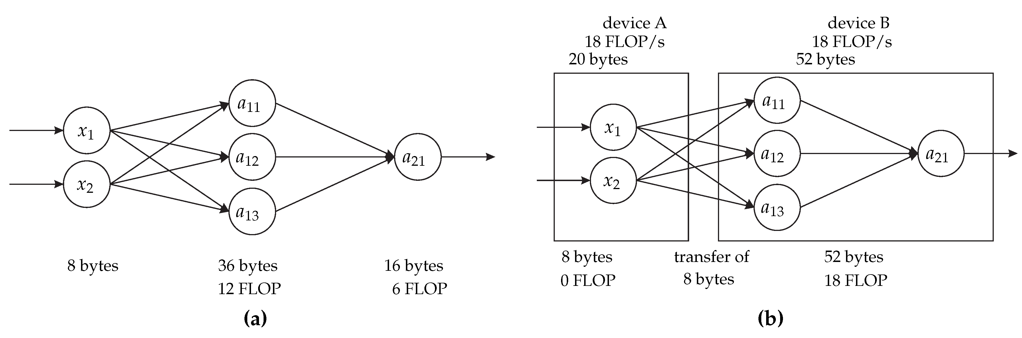
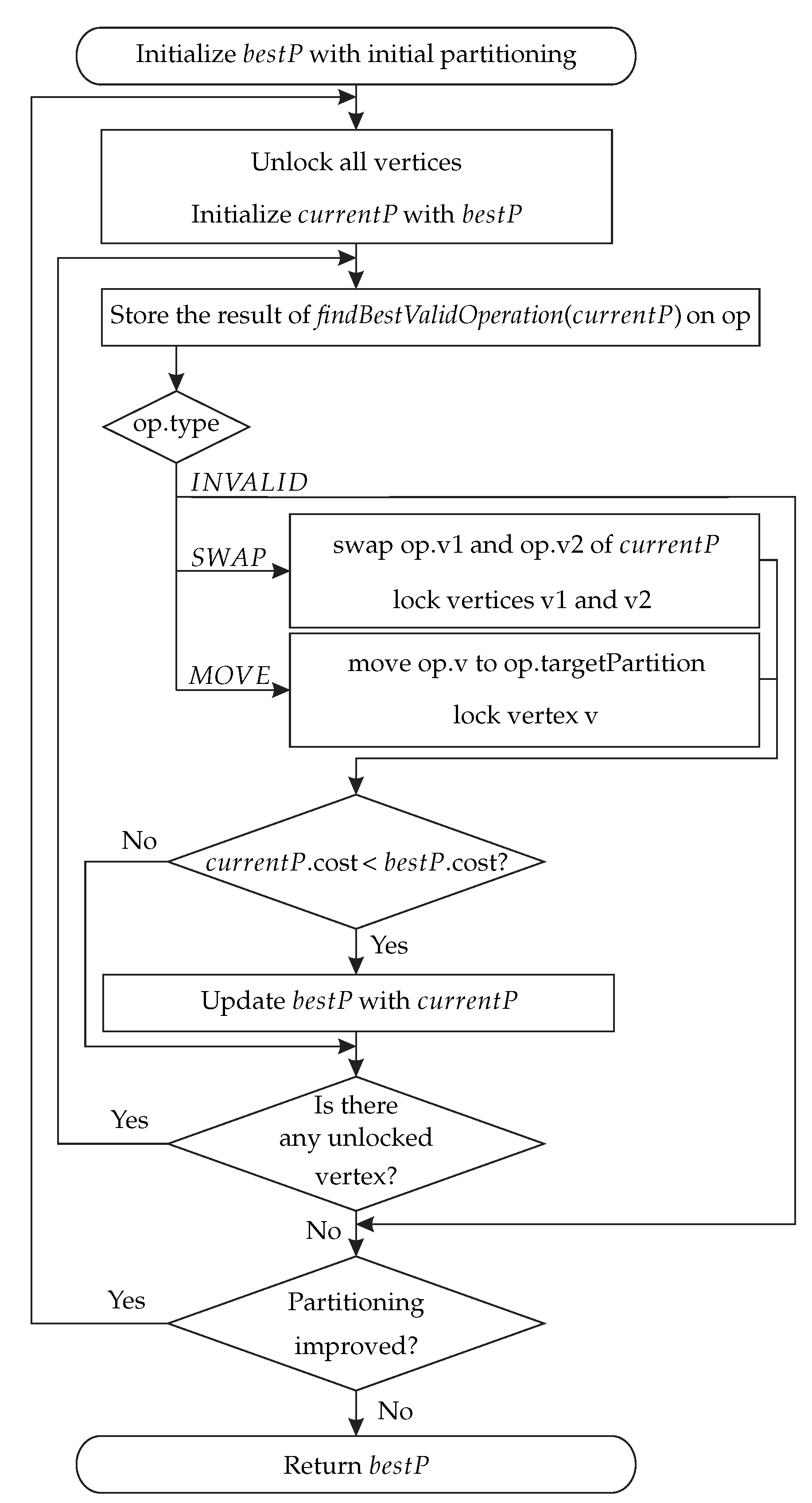
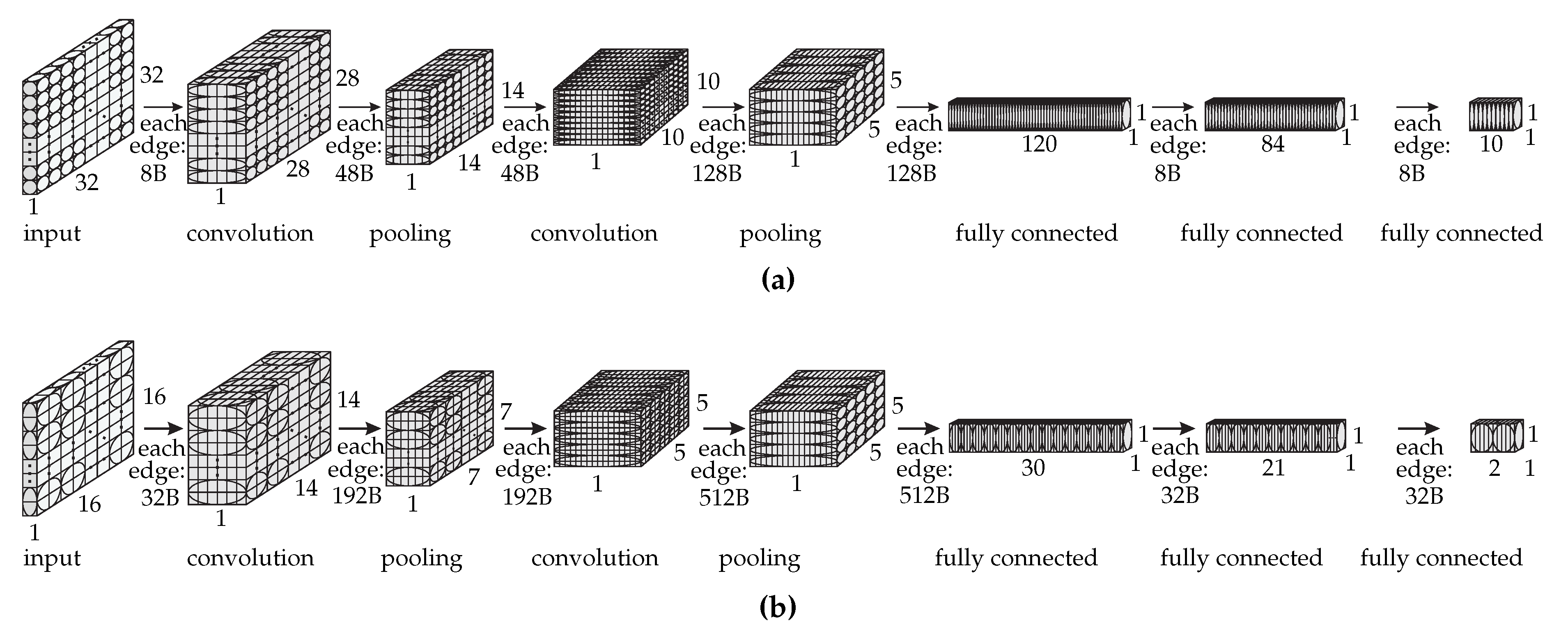
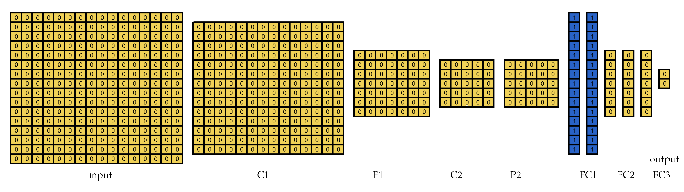
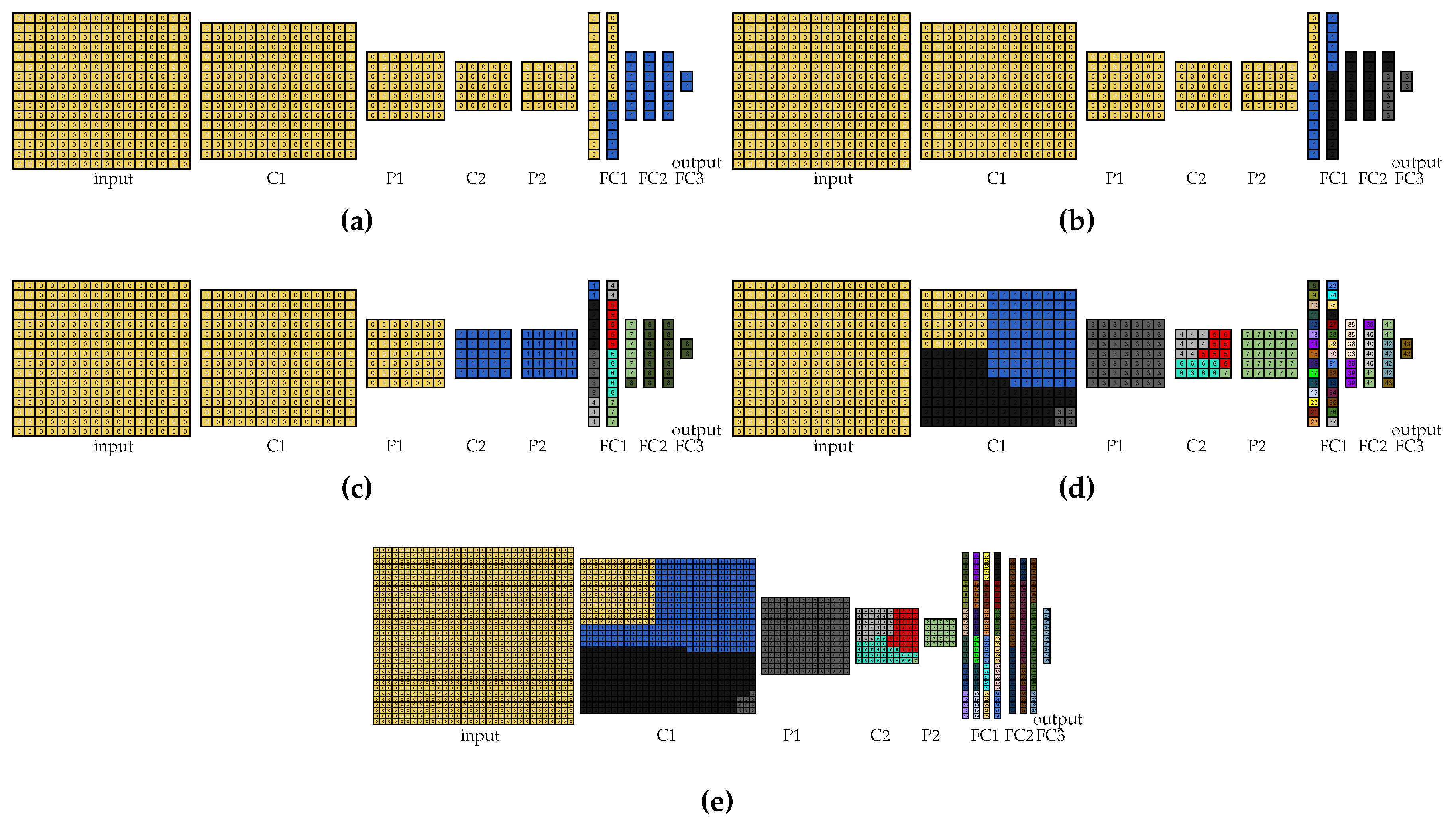
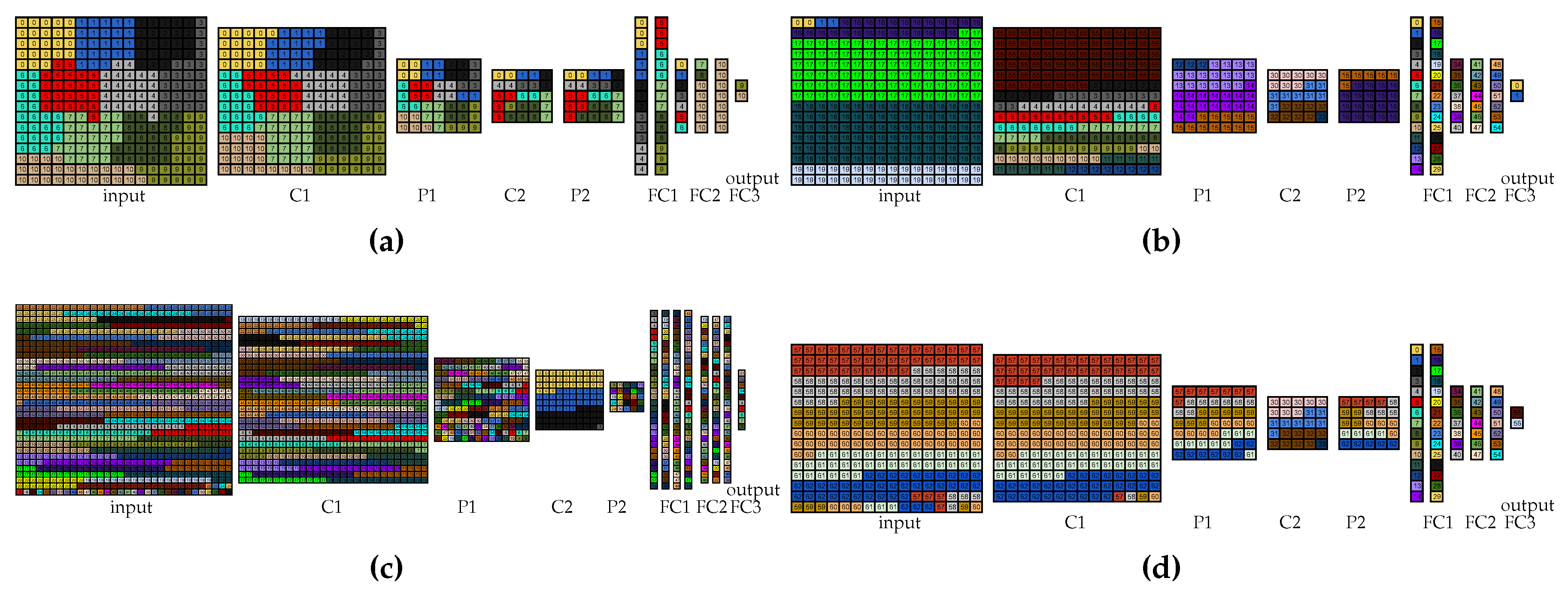
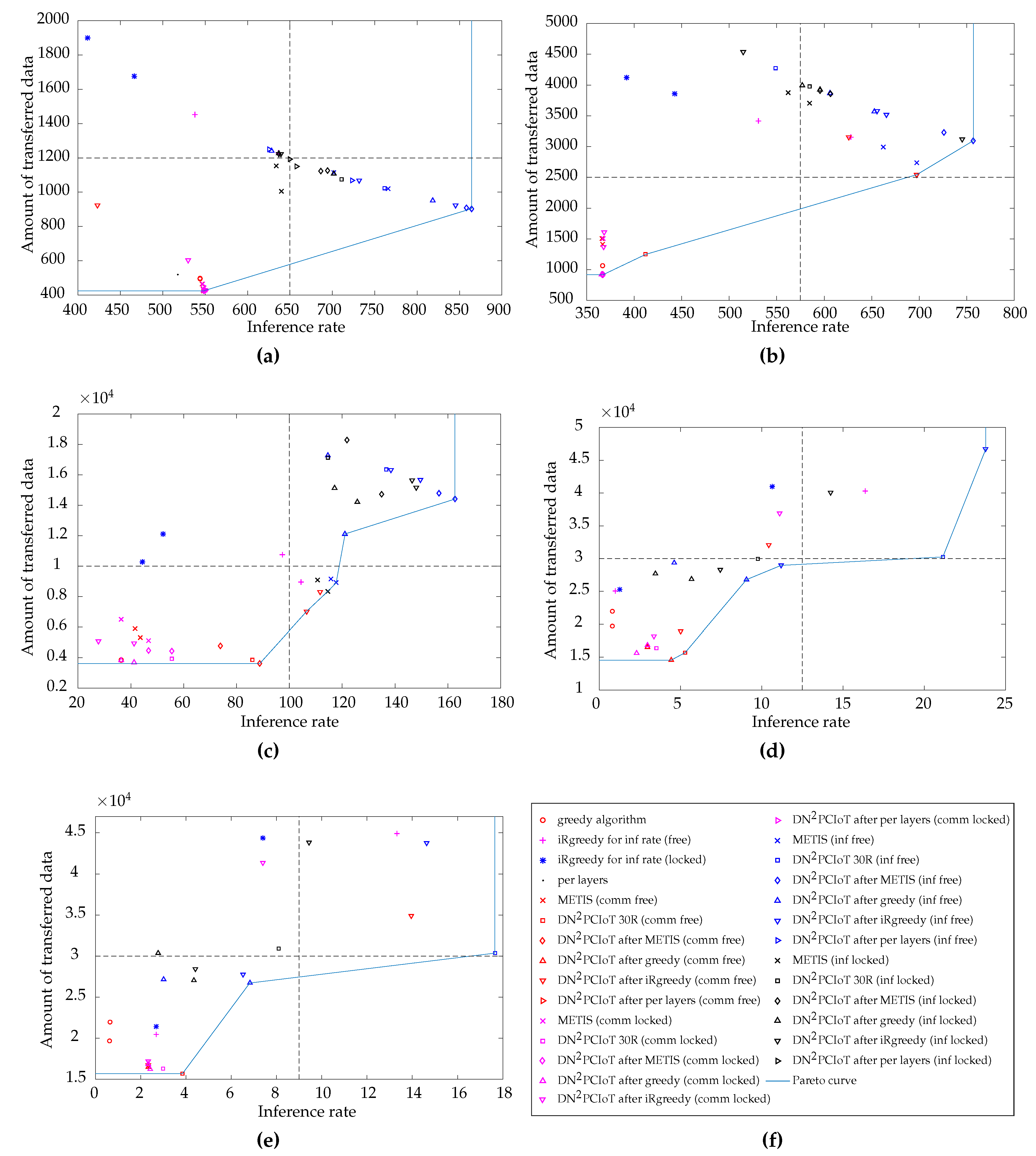
Table 1.
Summary of ML and IoT tools discussed in the related work.
| Approach | Reduce DNN to Fit Constrained Memory? | Loss of Accuracy? | Offload to the Cloud? | Partitioning Type | Type |
|---|---|---|---|---|---|
| Big-Little [8] | Yes | Yes | Yes | per layers | ML IoT |
| DIANNE [15] | No | No | No | per layers | ML IoT |
| DeepX [16] | Yes | Yes | Yes | per layers | ML IoT |
| TensorFlow [14] | No | No | No | per layers ** | ML |
| DeepIoT [13] | Yes | No | No | N/A * | ML IoT |
| Li, Ota, and Dong [31] | No | No | Yes | per layers | ML IoT |
| DeepThings [32] | No | No | No | along the neural | ML IoT |
| network layers | |||||
| Multifidelity [10] | Yes | Yes | No | N/A | ML IoT |
| Benedetto et al. [30] | No | No | Yes | per neurons | IoT |
* Not applicable. ** To use implemented functions.
Table 2.
Summary of partitioning algorithms discussed in the related work.
| Approach | Memory Constraints? | Partition Balance? | Eliminate Redundant Edges? | Objective-Function | Adequate Account of Shared Parameters? |
|---|---|---|---|---|---|
| SCOTCH [18] | No | With some load unbalancing | No | Reduce communication | No |
| KL [33] | Yes | With some unbalancing | No | Reduce communication | No |
| METIS [19] | No | With some unbalancing in the constraints | No | Reduce communication | No |
| Multilevel KL [37] | Yes | No | No | Reduce communication | No |
| JA-BE-JA-VC [39] | No | Yes | No | Balance partitions | No |
| Maximize | |||||
| Our approach | inference | ||||
| (DNPCIoT) | Yes | No | Yes | rate or | Yes |
| reduce | |||||
| communication |
Table 3.
Per-layer and per-vertex characteristics of each LeNet model used in this paper.
| Characteristic | Model | Input | C1 | P1 | C2 | P2 | FC1 | FC2 | FC3 |
|---|---|---|---|---|---|---|---|---|---|
| Memory of shared parameters and biases per layer (B) | both | 0 | 1248 | 96 | 12128 | 256 | 0 | 0 | 0 |
| Memory per vertex (B) | LeNet 1:1 | 8 | 48 | 48 | 128 | 128 | 3216 | 976 | 688 |
| LeNet 2:1 | 32 | 192 | 192 | 512 | 128 | 12864 | 3904 | 3440 | |
| Computation per vertex (FLOP) | LeNet 1:1 | 0 | 306 | 36 | 765 | 96 | 51 | 240 | 168 |
| LeNet 2:1 | 0 | 1224 | 144 | 3060 | 96 | 204 | 960 | 840 |
Table 4.
Device data and the maximum number of devices allowed to be used in the experiments.
| Number of Devices Allowed to Be Used in the Experiments | Device Model | Device Amount of RAM (KiB) | Device Estimated Computational Power (FLOP/s) | Communication Performance between Each Device (KiB/s) |
|---|---|---|---|---|
| 2 | STM32F469xx [43] | 388 | 6103.5 | |
| 4 | Atmel SAM G55G [44] | 176 | 3051.8 | |
| 11 | STM32L433 [45] | 64 | 332.9 | |
| 56 | STM32L151VB [46] | 16 | 11.9 | |
| 63 | STM32L151VB [46] | 16 | 9.4 |
Table 5.
Normalized results for the naive approaches. The minimum and maximum consider Table 5 and Table 6.
| Setup | Median of 30 Random | Per Layers 2:1 | Per Layers 2:1 | Greedy 2:1 | Greedy 1:1 | iRgreedy 2:1 | iRgreedy 1:1 | METIS 2:1 | METIS 1:1 |
|---|---|---|---|---|---|---|---|---|---|
| 2 free | 6.35 | 1.67 | 1.67 | 1.59 | 1.59 | 1.61 | 1.36 | 1.13 | 1.23 |
| 4 free | 4.09 | x | x | 2.06 | 2.06 | 1.43 | 1.21 | 1.09 | 1.14 |
| 11 free | 2.32 | x | x | 4.49 | 4.49 | 1.56 | 1.67 | 1.40 | 1.38 |
| 56 free | 2.12 | x | x | 29.25 | 29.53 | 24.00 | 1.45 | x | x |
| 63 free | 1.92 | x | x | 27.53 | 27.80 | 6.59 | 1.32 | x | x |
| 2 locked | 5.25 | 1.37 | 1.37 | 1.31 | 1.31 | 1.73 | 1.52 | 1.11 | 1.12 |
| 4 locked | 4.83 | x | x | 2.03 | 2.03 | 1.90 | 1.68 | 1.27 | 1.33 |
| 11 locked | 3.25 | x | x | 4.08 | 4.08 | 3.33 | 2.83 | 1.29 | 1.34 |
| 56 locked | 2.74 | x | x | 17.50 | 17.66 | 11.25 | 1.34 | x | x |
| 63 locked | 2.15 | x | x | 14.74 | 14.88 | 3.53 | 1.28 | x | x |
Table 6.
Normalized results for DNPCIoT 30R and DNPCIoT after approaches.
| DNPCIoT after | |||||||||
|---|---|---|---|---|---|---|---|---|---|
| Setup | 30R 2:1 | per Layers 2:1 | per Layers 2:1 | Greedy 2:1 | Greedy 1:1 | iRgreedy 2:1 | iRgreedy 1:1 | METIS 2:1 | METIS 1:1 |
| 2 free | 1.13 | 1.20 | 1.38 | 1.06 | 1.37 | 1.02 | 1.18 | 1.00 | 1.01 |
| 4 free | 1.38 | x | x | 1.16 | 1.25 | 1.16 | 1.14 | 1.00 | 1.01 |
| 11 free | 1.19 | x | x | 1.34 | 1.42* | 1.18 | 1.09 | 1.04 | 1.00 |
| 56 free | 1.12 | x | x | 2.62 | 5.14* | 2.12 | 1.00* | x | x |
| 63 free | 1.00 | x | x | 2.59 | 5.84* | 2.71 | 1.21* | x | x |
| 2 locked | 1.00 | 1.09 | 1.08 | 1.01 | 1.12 | 1.12 | 1.11 | 1.02 | 1.02 |
| 4 locked | 1.27 | x | x | 1.29 | 1.25 | 1.00 | 1.45 | 1.25 | 1.23 |
| 11 locked | 1.29 | x | x | 1.26 | 1.18 | 1.00 | 1.01 | 1.10 | 1.22 |
| 56 locked | 1.46 | x | x | 2.50 | 4.07* | 1.91 | 1.00* | x | x |
| 63 locked | 1.17 | x | x | 2.17 | 3.41* | 2.14 | 1.00* | x | x |
Table 7.
Pipeline parallelism factor for each experiment device.
| Setups | Single Device | Best Inference Rate | Pipeline |
|---|---|---|---|
| Inference Rate * | in the Experiments | Parallelism Factor | |
| 2x STM32F469xx | 507.265 | 864.22 | 1.70 |
| 4x Atmel SAM G55G | 338.177 | 757.03 | 2.24 |
| 11x STM32L433 | 225.451 | 162.65 | 0.72 |
| 56x STM32L151VB | 4.509 | 21.14 | 4.69 |
| 63x STM32L151VB | 4.509 | 17.65 | 3.91 |
* In the case that the device fits the memory required by the whole LeNet model.
© 2019 by the authors. Licensee MDPI, Basel, Switzerland. This article is an open access article distributed under the terms and conditions of the Creative Commons Attribution (CC BY) license (http://creativecommons.org/licenses/by/4.0/).
Share and Cite
MDPI and ACS Style
Martins Campos de Oliveira, F.; Borin, E. Partitioning Convolutional Neural Networks to Maximize the Inference Rate on Constrained IoT Devices. Future Internet 2019, 11, 209. https://doi.org/10.3390/fi11100209
AMA Style
Martins Campos de Oliveira F, Borin E. Partitioning Convolutional Neural Networks to Maximize the Inference Rate on Constrained IoT Devices. Future Internet. 2019; 11(10):209. https://doi.org/10.3390/fi11100209
Chicago/Turabian StyleMartins Campos de Oliveira, Fabíola, and Edson Borin. 2019. "Partitioning Convolutional Neural Networks to Maximize the Inference Rate on Constrained IoT Devices" Future Internet 11, no. 10: 209. https://doi.org/10.3390/fi11100209
Note that from the first issue of 2016, this journal uses article numbers instead of page numbers. See further details here.