Article

Effect of Climate Change Projections on Forest Fire Behavior and Values-at-Risk in Southwestern Greece

1
Department of Geography, University of the Aegean, 811 00 Mytilene, Greece
2
Institute for Environmental Research and Sustainable Development, National Observatory of Athens, 152 36 Athens, Greece
3
Navarino Environmental Observatory, Costa Navarino 240 01, Messinia, Greece
4
Research Center for Atmospheric Physics and Climatology, Academy of Athens, 106 72 Athens, Greece
*
Author to whom correspondence should be addressed.
Forests 2015, 6(6), 2214-2240; https://doi.org/10.3390/f6062214
Submission received: 21 January 2015 / Revised: 2 June 2015 / Accepted: 11 June 2015 / Published: 19 June 2015
(This article belongs to the Special Issue Climate Change and Forest Fire)

Abstract

:
Climate change has the potential to influence many aspects of wildfire behavior and risk. During the last decade, Greece has experienced large-scale wildfire phenomena with unprecedented fire behavior and impacts. In this study, thousands of wildfire events were simulated with the Minimum Travel Time (MTT) fire growth algorithm (called Randig) and resulted in spatial data that describe conditional burn probabilities, potential fire spread and intensity in Messinia, Greece. Present (1961–1990) and future (2071–2100) climate projections were derived from simulations of the KNMI regional climate model RACMO2, under the SRES A1B emission scenario. Data regarding fuel moisture content, wind speed and direction were modified for the different projection time periods to be used as inputs in Randig. Results were used to assess the vulnerability changes for certain values-at-risk of the natural and human-made environment. Differences in wildfire risk were calculated and results revealed that larger wildfires that resist initial control are to be expected in the future, with higher conditional burn probabilities and intensities for extensive parts of the study area. The degree of change in the modeled Canadian Forest Fire Weather Index for the two time periods also revealed an increasing trend in frequencies of higher values for the future.

Graphical Abstract

1. Introduction

Studies claim that global warming will eventually alter temperature and precipitation patterns around the world [1]. The trend in wildfire activity, according to climate and fire scientists, is expected to increase as the planet warms [1,2]. The impacts of climate change on wildfires might become more severe in the coming years due to the frequency of extreme weather events, rather than the overall change in the “average” climate patterns [3].
Changes in climate have the potential to significantly affect wildfire frequency, size and intensity; while higher fire risks, longer fire seasons and more severe fire effects are expected [3,4,5,6,7]. Therefore, these possible future changes on wildfire patterns will subsequently increase the risk of wildfire-related hazards and vulnerabilities such as microclimate alteration, floods, destruction of infrastructure, economic losses and human casualties. Many aspects of post-wildfire conditions will affect or accelerate other natural environmental disturbances, resulting in modified vegetation patterns and succession procedures, land degradation, desertification and hydrological cycle derangement. Even gradual and apparently small changes in climate can lead to catastrophic shifts in ecosystems when their resilience has been compromised by human exploitation [8]. Furthermore, carbon and other greenhouse gases emissions from wildfires cause feedback loops on the climate. An unfortunate feedback loop exists where more fires lead to greater emissions of greenhouse gases, leading to conditions increasingly conducive to wildfires [9,10,11]. The vulnerability of the Mediterranean region in anthropogenic climate change for the upcoming decades has been stressed in a number of articles (e.g., IPCC 2013 [12] and references thereafter). The redistribution of rainfall amounts is quite interesting in the complex topography of the Mediterranean in which areas with high precipitation are expected to receive less rainfall, while isolated regions such as the Aegean Sea show much less reduction of rainfall amounts in the future [13,14]. Studies of climate change for the Mediterranean region demonstrate the vulnerability of the area to human-made climate change, associated with a strong increase in temperature and decrease in rainfall [15,16,17,18,19]. Climate change indices for extreme events reveal changes especially in summer temperatures, where both minimum and maximum temperature extremes show statistically significant warming trends [20]. In addition, the number, intensity and length of heat waves were found to increase in the eastern Mediterranean region [21]. Future model predictions have shown that the number of days with maximum temperatures exceeding 35 °C and their total annual number are also expected to increase there [14,22]. Such changes may lead to an increase in the magnitude of forest fire risk in Greece and the eastern Mediterranean region.
The large fires that occurred in the Mediterranean Basin in the last decade were related not only to extremely warm and dry weather [23], but also to positive anomalies in the previous wet season that promoted plant growth and fuel build-up [24]. The large-scale wildfire events of Peloponnese, Greece, during the summer of 2007 raged for several days under the influence of high winds and low relative humidity, resulting in the most severe fire effects of the past 50 years [25]. The European Forest Fire Information System (EFFIS) reports that about 1500 fires broke out only in the Peloponnese peninsula in 2007, burning approximately 1000 km2 of land, 665 km2 of which was protected forests and natural areas [26]. According to the EFFIS dataset, the total burned area in Peloponnese for the 2000–2006 period was 540 km2, while based on the Hellenic Forest Service records, approximately 4500 major wildfires resulted in 2100 km2 of burned area from 1985 to 2004 [25]. Historical fire records and meteorological observations for Greece, spanning more than one century (1894–2010), revealed that fire occurrence, expressed as the annual number of fires and total burned area was strongly correlated with the mean maximum and the absolute maximum air temperatures [27]. Furthermore, Koutsias et al. [27] stated that the total burned area was strongly negatively correlated with fire-season precipitation, and positively correlated with two-year-lagged annual and summer precipitation, underlying the effect of precipitation in controlling fuel production and moisture.
The impacts of climate change on Mediterranean-type ecosystems may result from complex interactions between direct effects on water resources and subsequent modifications in flammability and fire regimes, leading to changes in standing biomass and plant species composition [7,28]. Fire regimes in the Mediterranean are influenced by factors beyond those related directly to climatic conditions (i.e., socioeconomics, land uses and intensive human pressures), but climate and weather conditions have a profound effect on fire behavior over time. Different vegetation types are anticipated to have different responses to climate change in terms of fuel availability and flammability. The removal of overstory vegetation and canopy cover will result in lower fuel moisture content and, thus, increased flammability.
Previous studies raised the question about the relative importance of weather and fuel on fire behavior, creating the “weather hypothesis” and the “fuel hypothesis” [29,30]. The weather hypothesis suggests that large, severe fires are driven by extreme weather events and intensely burn through forests regardless of the condition of their fuels; while on the contrary, the fuel hypothesis suggests that reduction of fuels limits fire severity. Forest fire behavior is complicated by the erratic and, often, weather-driven nature of these phenomena. Keeley and Fotheringham [31] claim that catastrophic fires are less dependent on fuel and more dependent on the coincidence with severe weather.
In this study, the weather hypothesis was applied by conducting fire behavior simulations of hard to control large wildfires that burn for five hours, based on data for present and future climate conditions derived from a Regional Climate Model (RCM). Key goals are to assess the degree of expected changes in the size, conditional burn probabilities and intensity of large wildfires that resist initial control efforts and to estimate the anticipated impact on values-at-risk in the area of Messinia in Peloponnese, Greece. Under the same context, the Canadian Forest Fire Weather Index’s (FWI) present and future RCM-derived values [32,33] were analyzed and statistically tested to identify trends and patterns of present and future fire risk.

2. Materials and Methods
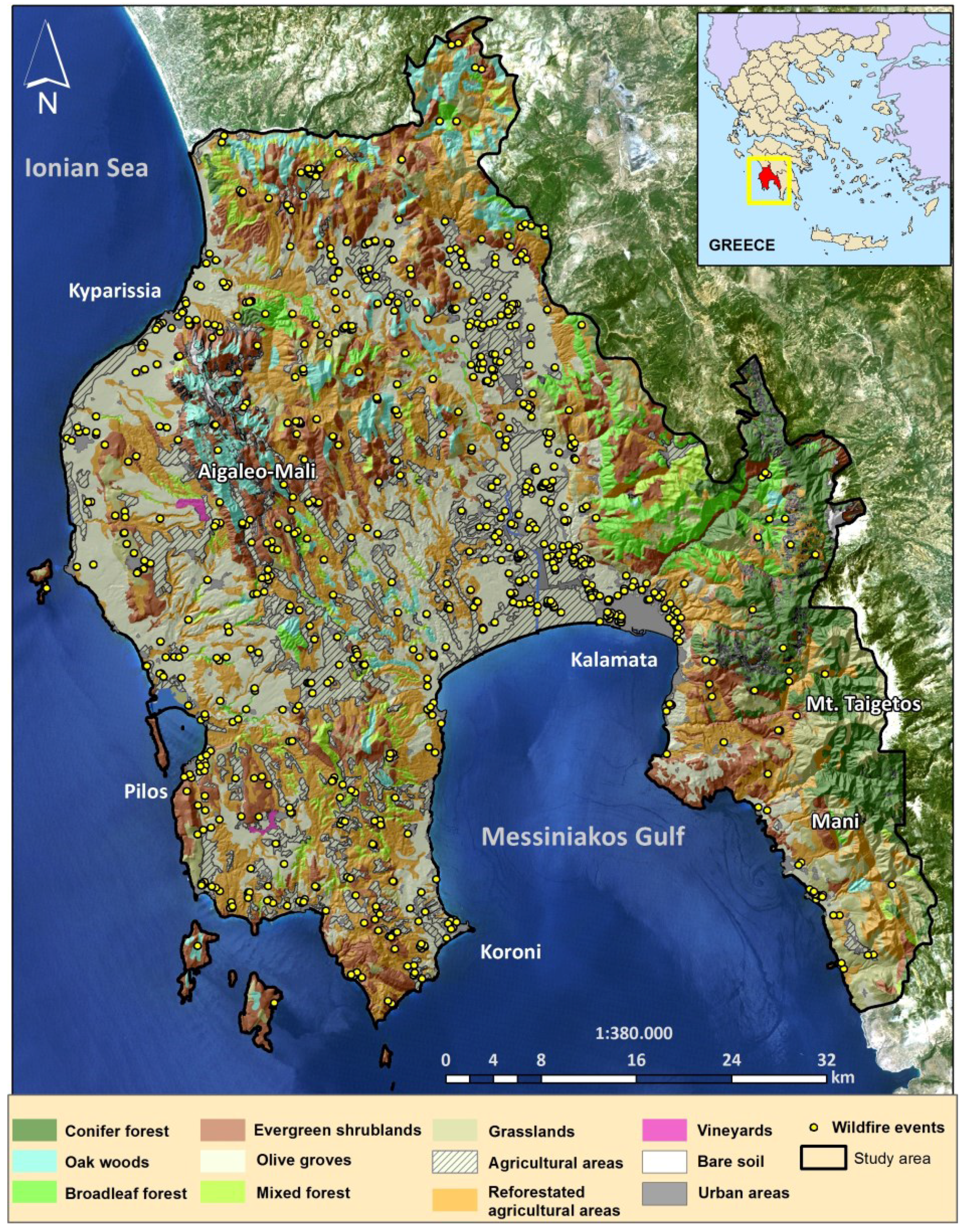
2.1. Study Area

Messinia, with a total area of about 3000 km2, is located on the SW and hazard-prone tip of Greece (with frequent earthquakes, floods and wildfires), having shores to the Ionian Sea (Figure 1). The average annual precipitation in this part of Greece ranges between 800 to 1600 mm over the elevation gradient [34,35]. During winter, the area is affected by the passage of depressions forming over the Mediterranean Sea, while in summer it is influenced by heat waves coming from N. Africa [36,37]. The steep and variable topography is creating local and diurnal wind patterns and forms local microclimates. Various archaeological sites of world importance (dated back to 2000 BC) exist on forested and densely vegetated areas. Furthermore, extensive wildland-urban interface (WUI) and rural-urban interface (RUI) areas can be found around the 500 towns, villages and settlements and, in conjunction with land abandonment and reforestation, increase the risk of human causalities from wildfires. The touristic infrastructure of the area is widespread across the coastline, where one of the largest hotel complexes of Greece is located. In addition, people tend to camp (legally or illegally) close or inside high fire risk areas during the summer season.
The vegetation of Messinia (Figure 1) encompasses 1150 km2 covered by evergreen shrublands, 250 km2 with grasslands and phryganic ecosystems, 140 km2 with oak woodlands (Quercus conferta, Q. ilex, Q. coccifera, Q. pubescens, Q. ithaburensis Decaisne ssp. macrolepis), 127 km2 with true-fir stands (Abies cephalonica), 116 km2 with broadleaf forests (Castanea sativa, Platanus orientalis, Acer pseudoplatanus, Sorbus domestica, Fraxinus ornus, Alnus glutinosa, Prunus cerasus) and 85 km2 with pine forests (Pinus halepensis, P. nigra ssp. pallasiana). The rest of the area is mainly covered by olive tree (Olea europaea) cultivations (600 km2) and agricultural areas (orchards, crops, vineyards, etc.).
About 6000 wildfire events were recorded during the 2000–2013 period from the Hellenic Fire Service [38], 92% of which burned areas less than 1 ha each, 7% burned between 1 and 10 ha each, 0.7% from 10 and 100 ha each and the 0.3% of wildfires burned more than 100 ha each. Almost all of these incidents were extinguished by firefighting forces, since no fires are left to burn without some kind of wildfire suppression. The majority of wildfire ignitions (52%) occurred during the June-September period, resulting in 96.7% of the total burned area. Regarding wildfire duration, 88% of all wildfire events were extinguished within five hours (33% within an hour), 8% lasted between 5 and 24 h, 3% lasted for more than a day, and only approximately 1% lasted for more than two days. There is evidence that quite a few ignitions are caused by lightning [39,40], but the vast majority initiated from agricultural practices, arson and accidents/negligence that are typical for Greece.
Numerous fire ignition points of the last 14 years have been mapped for this study, based on records from the Hellenic Fire Service, resulting in more than 800 significant fire events that burned forests and other lands (Figure 1). These records are rarely geo-referenced, so their location on the landscape is identified by the general toponym of the area where the fire was ignited. As a result, only a portion of the total ignitions can be identified and mapped (i.e., large wildfires or those few records with adequate details). The recorded wildfires resulted in about 24,000 ha of burned lands, while the mapped ignition points represent burned areas of approximately 23,000 ha, capturing most of the area burned. Finally, the use of several different satellite images enabled the identification and mapping of 68 wildfire perimeters, with the 50th, 80th, 95th and 98th percentiles representing burned areas of 27, 151, 986 and 7233 ha respectively (the minimum mapping size was 4 ha).
Figure 1. Land use/land cover types and fire ignitions from 2000 to 2013 in Messinia, Greece.
Forests 06 02214 g001

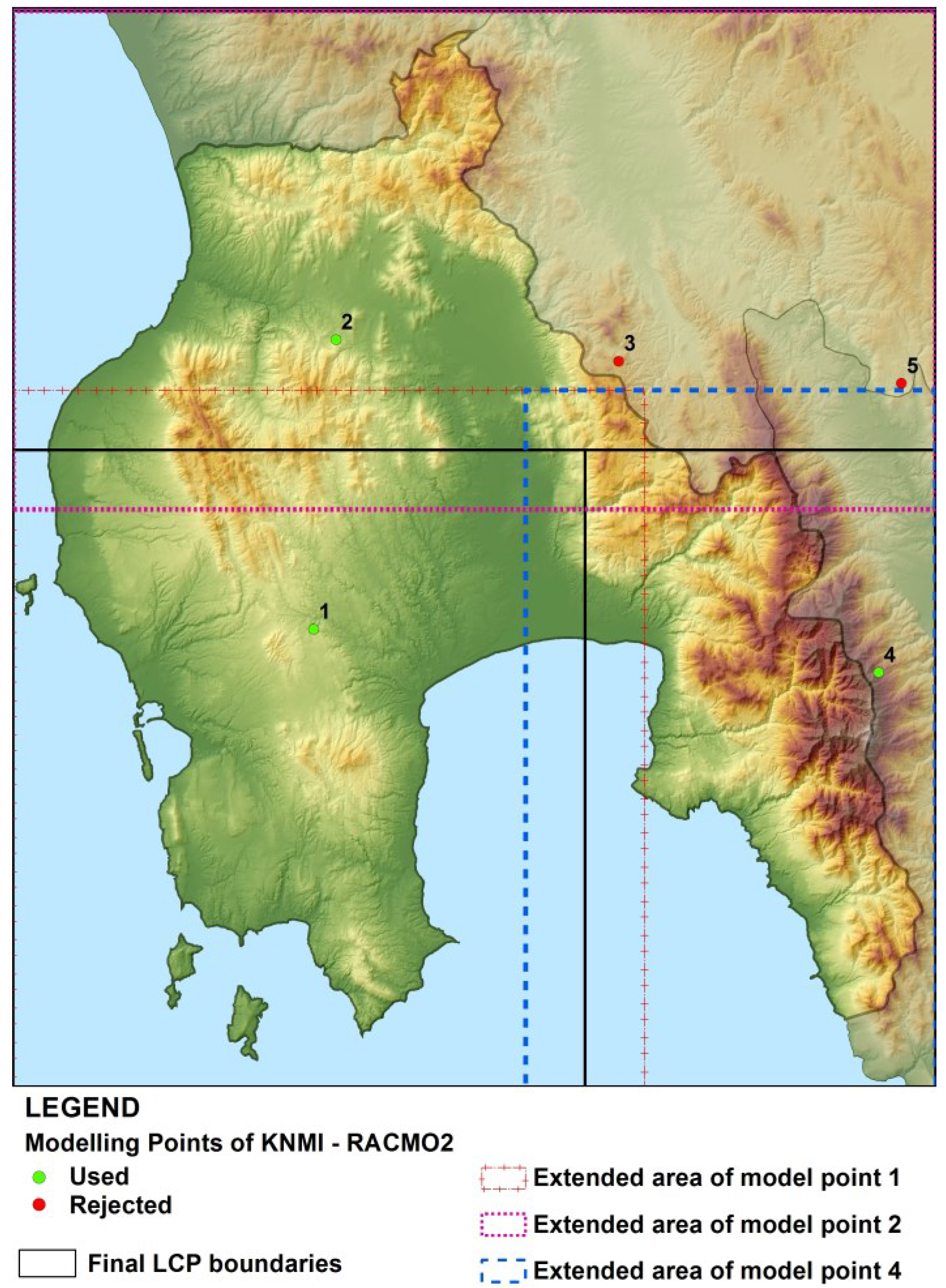
2.2. Simulation Inputs and Software

To assess climatic changes related to fire risk in the study area, daily outputs from the KNMI RCM RACMO2 [41,42,43,44] were used. The KNMI RACMO2 is forced with output from a transient run conducted with the ECHAM5 Global Climate Model (GCM), with a spatial resolution of about 25 × 25 km under the SRES A1B emission scenario [45]. The SRES A1B emissions scenario is a medium-to-high emission scenario in terms of greenhouse gas emissions affecting the world’s climate. ECHAM5 GCM lies in the middle of other global models for the same A1B scenario. Hence, we expect that the results of this model are on the average side for the study area.
KNMI RACMO2 RCM has been extensively validated throughout Europe (including the Mediterranean region) in the context of the EU project ENSEMBLES (www.ensembles-eu.org). This model was selected amongst several other available, as it was the best performing model for the region; and thus, this model was used as the input of our study [46,47]. According to these cited publications, KNMI-RACMO2 was found to simulate the mean climate and the extremes in Europe and the Mediterranean region with more accuracy. Furthermore, a regional evaluation of various models (including KNMI RACMO2) for the Balkan Peninsula focusing on climate extremes proved that the KNMI RACMO2 manages to reproduce patterns of extreme temperature and precipitation with reasonable accuracy when compared to the E-OBS gridded observational dataset [19].
The model provides five grid points over SW Peloponnese, three of which were used in this research (Figure 2; i.e., green dots for Points 1, 2 and 4). Points 1 and 2 were used because they fall exactly within the study area; Point 4 was additionally used for it represents the high elevation parts of the study area. Having closely examined the RCM outputs, we figured that Point 3, located on a medium-elevated area, is very close to the average of Points 2 (which is relatively flat terrain) and 4. Hence, we decided that Points 3 and 5 (which is far outside the study area) would not provide any new insights to our analysis and were not used in the calculations. Points 1, 2 and 4 were also used to delineate the three landscape files (LCP) of the study area; LCP is a binary file comprised of a header and a body of short integers for each of the themes it contains (topographic and vegetation spatial input layers), used in some wildfire simulation software.
Simulations of present-day (period 1961–1990) and distant-future (period 2071–2100) parameters were utilized including relative humidity (%), mean and maximum temperature (°C), wind speed (m/s) and the mean eastward (u) and northward (v) wind components. The u and v components were used to calculate the wind direction, as derived from arctan (u/v), and averaged for 16 directions. Wind speed and direction were calculated at the height of 10 m above ground level, while air temperature and relative humidity at 2 m above sea level, with no scaling of values to the elevation of the ground surface.
Mean RCM-derived daily values of maximum air temperature, relative humidity, wind speed and 24 h accumulated precipitation for the present and future time periods were used to calculate daily fire risk values, represented by the FWI. The FWI is part of the Canadian Forest Fire Danger Rating System that is used worldwide for the estimation of wildfire risk in a generalized fuel type [32,48]. The FWI is a non-dimensional index that is based on physical processes, and its calculation requires inputs of weather readings taken at noon standard time to rate the wildfire risk at the mid-afternoon peak (from 14:00 to 16:00 h). The meteorological variables required for the index calculation are air temperature, relative humidity (in the shade), 10 min average wind speed (at 10 m above ground level) and 24 h rainfall. The Canadian Forest Fire Weather Index System consists of six components: i.e., three fuel moisture codes (Fine Fuel Moisture Code, Duff Moisture Code and Drought Code) and three fire behavior indices (Initial Spread Index—ISI, Buildup Index—BUI, and FWI). Information from the ISI and BUI are combined to provide the numerical rating of fire intensity into FWI that is categorized into four fire danger classes (FWI < 8: low; FWI ≥ 8 and FWI < 17: medium; FWI ≥ 17 and FWI < 32: high; and FWI ≥ 32: extreme). The FWI has been widely tested and applied successfully across the Mediterranean Basin [49,50,51,52,53,54,55]. To avoid overlapping results, only one point from the RACMO2 model’s outputs was used as representatively for the subsequent FWI statistical analysis; i.e., Point 1 (SW Messinia) covering the area where the majority of people and values-at-risk are located (Figure 2). Furthermore, after the calculation of the number of days with elevated fire risk (i.e., days with FWI ≥ 32) for all RCM grid points covering an extended area of southwestern Greece, maps were excerpted to portray the changes between the present and the future in the Messinia region, by implementing Kriging interpolation similarly to previous research [55].
Figure 2. The five prediction points of KNMI RCM RACMO2 model and influence areas of the three used Points 1, 2 and 4 (green) over Messinia, Greece.
Forests 06 02214 g002
For the quality assessment of the RCM data, a comparison of FWI values calculated using historical observations vs. FWI values calculated using model outputs (ensemble mean of the model for the nearest grid point) for the present period (1961–1990) was performed. Two sites with the available set of observational data were used: one in southeastern Attica (Sounio) and the other in the western part of Peloponnese (Andravida) (source: Hellenic National Meteorological Service). The calculation of FWI was performed for the wildfire season (May to October). Model outputs slightly underestimate FWI values during May and June, while an overestimation occurs for the rest of the months. Throughout the May-October period, the RCM calculated FWI values are consistent and indicative of the actual FWI trend, catching both the value increase (May to July) and decrease (August to October), as well as the peak values of July and August.
FWI is sensitive to changes in the meteorological parameters used in its calculation, and those with the highest impact on the index are precipitation and wind speed (see Figure 3 in [55]). In Greece, even for moderate wind speeds, the index exceeds the critical risk thresholds. For gale force winds, frequent in eastern Greece during the summer, the index reaches extremely high values. As temperatures rise, FWI substantially increases with higher wind speeds. Conversely, even a minimum amount of rain on the previous day can reduce FWI values by 80%, generally dropping them below the specified critical risk thresholds.
Figure 3. Fire season monthly FWI values for the present (blue) and future (green) time periods.
Forests 06 02214 g003
Fire behavior simulations were conducted by the command-line version of the Minimum Travel Time (MTT) algorithm [56], called Randig [57], making it feasible to rapidly simulate thousands of fires. These numerical simulations are stochastic, which means that they are conducted in a way that inherently incorporates uncertainty and variability in the simulation inputs. For this study, the sources of stochasticity of Randig simulations were the random fire ignition locations; which then were modeled with a random selection among several predefined weather scenarios and with randomness on how many of the nodes with initiated crown fire can actually launch embers that may start new fires. MTT searches for the fastest path of fire spread among nodes in a two-dimensional network, and then the paths producing minimum travel time between nodes are interpolated to reveal the fire perimeter positions at an instant in time [56]. Calculations can generate fire growth in the absence of time-varying winds or fuel moisture content, which enables analysis only of the effects of spatial patterns of fuels and topography [58]. Fire spread is based on Huygens’ Principle, where the growth and behavior of the fire edge is a vector or wave front [56,59].
Randig results include a conditional burn probability grid of the area, representing the conditional likelihood that a cell will burn given a certain set of ignitions, fuel moistures and wind speeds/directions, similar to the historic fires [60]. The absolute problem-fire burn probability at a cell has little inherent meaning and cannot be compared across different assessment landscapes. Additional outputs are the fire perimeter shapefiles, conditional flame length probability and a fire list (text file with coordinates and burned area of each fire). Conditional burn probability (CBP) is defined as (1):
C B P = F B / n
where, FB is the number of times a cell burns and n is the number of simulated fires.
Flame length probabilities are calculated in 20 classes (0.5 m interval). The fireline intensity (FI—kW/m) for a given fuel type and moisture condition can be calculated from the fire spread rate normal to the front [61,62], and then it is converted to flame length (F—m) based on Byram’s [61] Equation (2):
F = 0.0775 × F I 0.46
Conditional flame length (CFL) is the probability weighted flame length given a fire occurs and acts as a measure of wildfire hazard [63], while it is calculated by incorporating the flame length distribution generated from multiple fires burning each cell in Equation (3):
C F L = i = 1 20 ( B P i B P ) ( F i )
where, BP is Burn Probability and Fi is the flame length midpoint of the ith category.
Randig uses an LCP file, similar to FARSITE [64] and FlamMap [59]. Topographic spatial inputs (i.e., elevation, slope and aspect) were derived from ASTER GDEM V2. Extensive field sampling was conducted on the study area on over 250 sites to record vegetation types, fuel models, crown base height (CBH) and stand height. The main fuel modeling scheme was based on Scott and Burgan’s [65] standard fuel models, supplemented by some custom fuel models designed for Greece [66,67]. Several vegetation types that are typically considered non-burnable (e.g., orchards, vineyards, olive groves, agricultural areas), were identified in the fieldwork that are not maintained in a non-burnable condition and there is enough dead fuel to sustain a surface fire (grass that is allowed to grow beneath vines, olive trees and orchard trees), even with very low spread rates and intensity. However, there were parts of the study area that these vegetation types were non-burnable, and as a result, different fuel models were used. By visual interpretation and digitization over aerial orthophotos, canopy cover was categorized into the coverage classes supported by FARSITE and FlamMap (0–4). CBH and stand height were attributed per stand or polygon level, based on field records (average or dominant value). In a similar way, crown bulk density was attributed based on values derived from literature, combined with the coverage of each stand [68,69,70,71,72]. All the spatial inputs of LCP file have a cell size of 30 m.
Randig accepts weather parameter inputs in the form of scenarios that define wind speed and direction (mph at 20 feet above ground level), dead and live fuel moisture content (FMC) for each fuel model and the selection probability of each scenario. To define these scenarios for Messinia, the daily wind speeds of each time period were sorted into three classes (0 to 2 m/s, 2 to 4 m/s and greater than 4 m/s) that are based on the RCM wind data of the region during the high wildfire risk season (from June till the end of September). Then, the percentage of days that fall in each category over the total number of prediction days, as well as the wind direction frequency (%) per sector was calculated. The three most frequent wind direction sectors were used for each wind speed category, with their frequency been used for defining the selection probability of every scenario on Randig simulations. Eventually, each time period has had nine weather scenarios (three wind speeds with three directions each), with the relevant FMC values for each wind speed category (Table 1). It is evident that differences in the number of days of each wind speed category are relatively small, with wind direction frequencies being the most variable and FMC values having an important change.
Table 1. Weather outputs from RCM RACMO2 used to create the weather scenarios input files for Randig simulations. A1, A2 and A4 are the three RCM prediction points; P: Present; F: Future; Fuel moisture values represent 1 h, 10 h, 100 h, live herbaceous and live woody fuel moisture content classes, respectively.
Wind Speed Category% of DaysDominant DirectionsExposed Fuel MoistureShaded Fuel Moisture
5 mph-A1-P51.91SE/26.9%SSE/22.6%S/13.7%6/7/8/60/909/10/11/90/120
5 mph-A1-F51.28SE/30.0 %SSE/18.5%ESE/16.6%5/6/7/30/608/9/10/60/90
10 mph-A1-P40.22SE/62.8%ESE/10.1%SSE/9.7%6/7/8/60/909/10/11/90/120
10 mph-A1-F41.07SE/63.6%ESE/11.0%S/8.3%5/6/7/30/608/9/10/60/90
18 mph-A1-P7.87SE/75.3%ESE/12.2%SW/3.5%6/7/8/60/909/10/11/90/120
18 mph-A1-F7.65SE/80.7%ESE/9.6%SSE/2.1%6/7/8/30/609/10/11/60/90
5 mph-A2-P76.07SE/27.6%ESE/16.6%SSE/12.6%6/7/8/60/909/10/11/90/120
5 mph-A2-F74.86SE/27.3%ESE/20.6%SSE/12.5%5/6/7/30/608/9/10/60/90
10 mph-A2-P22.35SE/39.0%ESE/37.0%SSW/5.7%6/7/8/60/909/10/11/90/120
10 mph-A2-F23.69ESE/40.0%SE/35.9%SSW/6.5%6/7/8/30/609/10/11/60/90
18 mph-A2-P1.58ESE/41.4%SW/17.2%SE/15.5%6/7/8/60/909/10/11/90/120
18 mph-A2-F1.45ESE/45.3%SW/20.8%SE/15.1%6/7/8/30/609/10/11/60/90
5 mph-A4-P74.18SSW/23.3%SE/14.9%ESE/13.7%5/6/7/60/908/9/10/90/120
5 mph-A4-F75.46SSW/22.7%ESE/14.3%SE/13.9%4/5/6/30/607/8/9/60/90
10 mph-A4-P24.32SSW/38.9%ESE/24.8%E/13.6%5/6/7/60/908/9/10/90/120
10 mph-A4-F22.90SSW/45.7%ESE/24.5%E/12.8%4/5/6/30/607/8/9/60/90
18 mph-A4-P1.50SW/67.3%SSW/25.5%E/5.5%4/5/6/60/907/8/9/90/120
18 mph-A4-F1.64SSW/51.7%SW/45.0%E/1.7%3/4/5/30/606/7/8/60/90
To estimate FMC, the relative mean air temperature and relative humidity values from each wind scenario were incorporated into the BehavePlus software [73], using the “Fine Dead Fuel Moisture Tool” to estimate the FMC for the 10 h diameter class (0.64 to 2.54 cm). Key findings from RCM outputs suggest that the average percent change (future vs. present) for average and maximum temperature and relative humidity are +19.2%, +16.4% and −11.6%, respectively, for Point 1; +20.6%, +16.8% and −12.1% for Point 2; and +21.3%, +17.9% and −14.8%, respectively, for Point 4. The calculations were based on tables published by Rothermel [74]. The tool’s defined input parameters (in parentheses) are the time period (May, June and July), time (12:00–13:59), slope (0–30%), aspect (south) and a choice for the calculation of FMC values on either shaded (≥50% shading) or exposed to sunlight fuel models (<50% shading). If the change of weather parameters between the two time periods was not very large, then the derived 10 h FMCs were the same, since Rothermel has grouped air temperature and relative humidity values at certain range classes.
Records from three weather stations with 10 h fuel moisture sticks installed on them (from another part of Greece with similar climate and fuels; http://meteo.aegean.gr), revealed that the average FMC difference between July and August is approximately 0.3%, while the decrease from June to July is 1.5%–2% and the increase from August to September is 2%–2.5%. These findings suggest that for the two months of July and August with the vast majority of wildfire ignitions, FMC variability is low.
For 1 h (0–0.64 cm) and 100 h (2.54 to 7.62 cm) FMC diameter classes, a value of 1% was subtracted and a value of 1% was added on the derived 10 h value, respectively. Randig has the ability to use different FMC values depending on fuel model type. Fuel models were sorted as either shaded or exposed (Table 2). For live FMC (herbaceous and woody), the values of 60%/90% (2/3 cured herb) and 90%/120% (1/3 cured herb) were attributed on exposed and shaded fuel models, respectively, for the present-day period; while for the future period, these values were modified as 30%/60% (totally cured) and 60%/90% (2/3 cured herb), respectively. The main assumption to derive the live FMC values is that they would change to the next driest category in the future. Each weather scenario had its own FMC file.
Table 2. Land use/land cover types, fuel models with the relevant codes and shading condition.
General Vegetation TypeFuel ModelFuel CodeShadedReference
Orchards and vineyardsGR1/NB9101/99NoScott and Burgan [65]
Olive groves and WUIGR2/NB9102/99NoScott and Burgan [65]
Agricultural areasGS1/NB9121/99NoScott and Burgan [65]
Abandoned and reforested agricultural areasGS2122NoScott and Burgan [65]
Sparse oak forestSH4144NoScott and Burgan [65]
Mixed forests and shrubsSH5145NoScott and Burgan [65]
Pine reforestationSH6146NoScott and Burgan [65]
Brush and grass ( phrygana)AS01206NoDimitrakopoulos and Panov 2001 [67]
Sparse shrubsSC01208NoDimitrakopoulos and Panov 2001 [67]
ShrubsSC02209NoDimitrakopoulos and Panov 2001 [67]
Oak forestTU1161YesScott and Burgan [65]
Fir forestTU3163YesScott and Burgan [65]
Mixed forestTU5165YesScott and Burgan [65]
Plane trees and chestnutsTL2182YesScott and Burgan [65]
Mixed oak with Quercus ilexTL6186YesScott and Burgan [65]
Broadleaf forestTL9189YesScott and Burgan [65]
Pinus nigraFM03212YesPalaiologou et al. 2013 [66]
Pinus halepensisFM02211YesPalaiologou et al. 2013 [66]
Non-burnable areasNB91–99-Scott and Burgan [65]
All the above values were grouped into new input files required for Randig execution, one for each prediction point and time period, resulting in a total of six input files. Additional required inputs were the fire simulation duration (300 min) (i.e., the duration of the fire growth calculations for the set of constant fuel moisture and wind conditions), spot probability (0.1) (a setting of 1.0 will compute a spot distance and direction for each crown fire node and a setting of 0.0 will prevent any spot fires), number of weather scenarios per fire (1) (i.e., how many different weather inputs can be used for each fire simulation) and spatial resolution of calculations (60 m). The vast majority of 2000–2013 wildfire events (88%) were extinguished within 5 h, so it was assumed that 300 min is a reasonable and representative wildfire duration. Tests with Randig revealed that an increase in wildfire duration produced very large burned area per fire with large CBP values. On the contrary, tests with small wildfire duration (1 h, i.e., 33% of the 2000–2013 recorded wildfire events) revealed that the produced wildfire sizes were not adequate to burn at least once each non-burnable cell of the study area (~30% of burnable pixels), as suggested on several Randig implementation studies [63,75]. Results revealed that with the defined duration, only the 3.48% and 1.54% of the burnable pixels for present and future periods, respectively, did not burn at least once. MTT is well suited to short-range assessments of fire growth, where weather conditions could be assumed constant (e.g., several hours) [56].
The simulated fires per prediction point was set to 100,000; i.e., an adequate number to saturate the landscape and ensure that, in conjunction with wildfire duration, the burnable pixels that do not experience even a single wildfire are the minimum possible. The same number of wildfire ignitions was used for the three LCPs. Fire ignition points were randomly located across the landscape by using an ignition probability grid that was produced by applying the kernel density estimation on the 800 mapped wildfire events. For crown fire simulations, the method proposed by Finney (1998) was set [64], due to the fact that from previous research on the study area [76] there was strong evidence that Scott and Reinhart’s crown fire method simulated large fires with more spotting [77]. Since several reports and observations from the study area suggest that wildfires commonly produce new ignitions through spotting, it was reasonable to set a value above zero, not too high (increased simulation time) and not too low. The spatial variation of wind speed and direction was simulated by enabling the WindNinja algorithm [78], using the weather scenarios as inputs. Burn period, spot probability and fire number were intentionally kept constant for all simulations (present and future) so that the differences of output values would be mainly the result of wind and moisture parameters. By keeping the duration constant, we were able to directly compare fire sizes between the different simulations. Randig simulation results must be contextualized as the uncontained wildfire growth in the absence of any firefighting effort.
The three selected prediction Points (1, 2 and 4) cover the SW, N and SE parts of Messinia, respectively (Figure 2). The regions corresponding to the area closer to each point were initially derived using the Thiessen polygons calculation method and the results were reformed to parallelogram shapes around each point. Due to the fact that Randig simulations do not expand to no-data cells, areas close to the LCP edges would have unrealistic/error values. To resolve this issue, the derived areas were expanded by 5 km inside Messinia to create three LCP files. Randig results were clipped by the initial defined area and then merged to form the final files of present and future time period simulations.
By using spatial data and information for values-at-risk, such as houses outside urban areas, agricultural infrastructures (corrals, residential storehouses, auxiliary buildings, etc.), hotels, wildlife habitats, monuments, industries/businesses and wildland-urban interface areas, a vulnerability assessment analysis was conducted for each of them for the two time periods. Randig results (CBP and CFL) are displayed as hex-binned scatterplots for each value-at-risk, indicating those attributes that have the potential of facing larger and/or intense fires. An extension of ArcGIS 10 [79] called ArcFuels [80] was used for the post processing of Randig results. The spatial data for values-at-risk must be in polygon format to estimate the average CBP and CFL values around them; thus, buffer zones were created for houses, hotels, WUI, industries, agricultural infrastructures and monuments (50, 300, 1000, 100, 50 and 100 m, respectively). No additional processing was needed for wildlife habitats. This analysis allowed the identification of important attributes with respect to high vulnerability (e.g., hotels, houses, etc.).

3. Results and Discussion

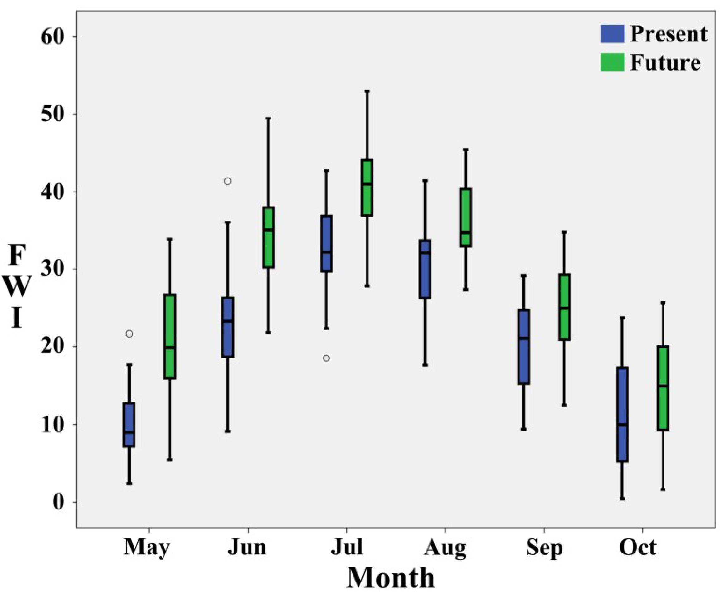
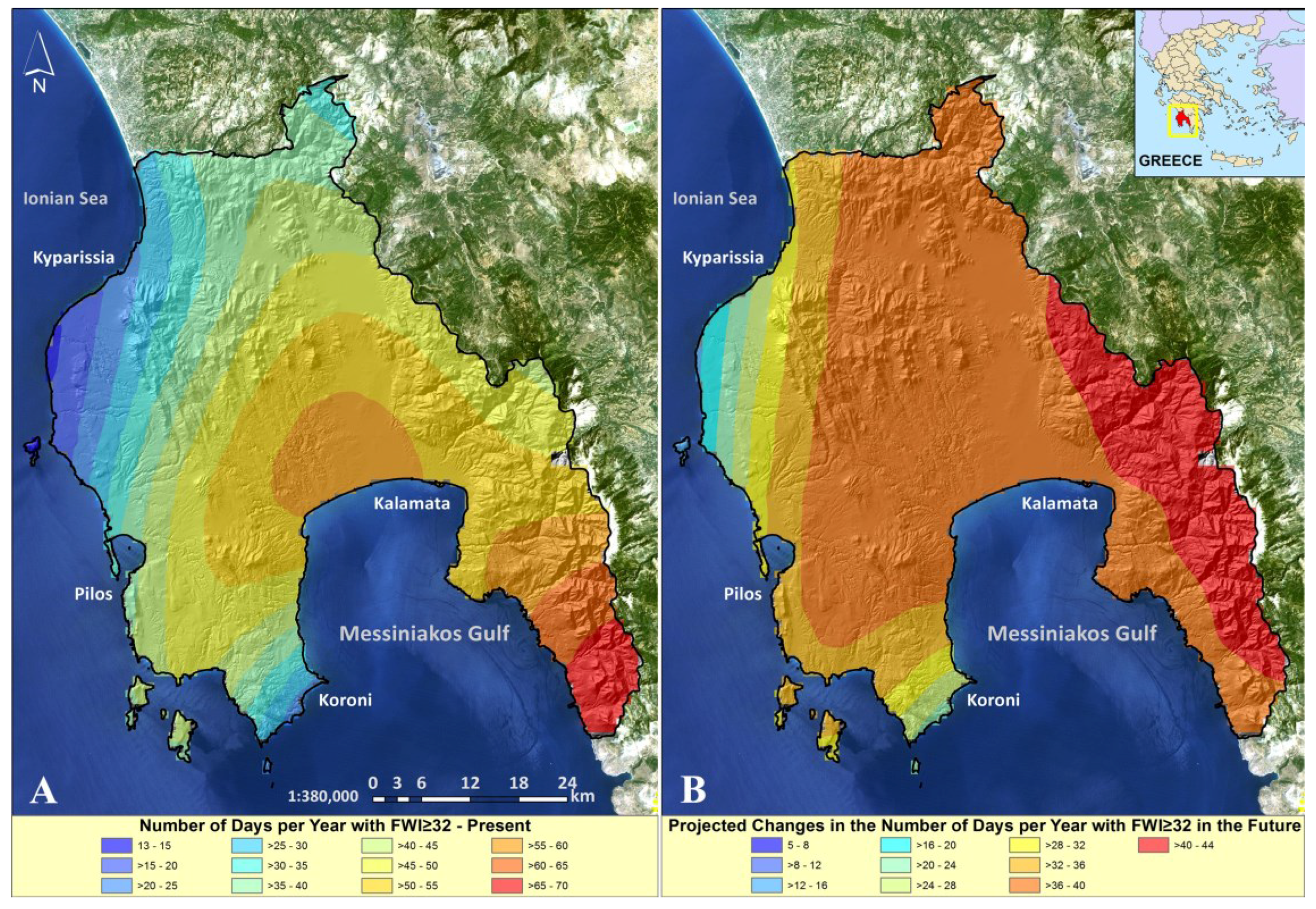
3.1. Fire Weather Index

Results from FWI statistical analysis (Table 3) reveal the differences among fire season months for the RCM-derived FWI values of present and future time periods. The mean and median values for all months show an increase for the future time period. For all months, statistical results revealed that the means of the two time periods are statistically significantly different (t-value), with differences ranging from 3.6 (October) to 11.3 (June). Furthermore, the number of days with low FWI class shows a reduction in the future ranging from −100% (July) to −27.3% (September). The same pattern applies for the medium FWI class, where the decrease ranges from −92% (July) to −31.5% (September), with the exception of October where a slight increase (4.5%) is noticed. The high FWI class portrays lower decrease rates, with the exception of May and October having a 238.1% and 63.2% increase, respectively. The number of days with extreme FWI class shows large increases, ranging from 44.3% (August) to 1320% (May), with the exception of October that remains the same between the two time periods. It is also evident in Table 3 that the future daily FWI values for the selected fire season months are higher compared to the present values (F > P) by a range of 61 to 81% of the total observations. In Figure 3, the monthly FWI box plots are displayed for the two time periods, and the increase of future average monthly and percentile values is evident.
To assess the influence of FWI on wildfire ignitions, a dataset was created with 2576 days of the months May to October for the 2000–2013 period (971 ignitions and 1605 no-fire days), which is the only period available with an adequate number of wildfire observations (Hellenic Fire Service records). An independent-samples t-test was conducted to compare FWI values in fire and no-fire days. There was a significant difference in the scores for fire (M = 24.48, SD = 12.54) and no-fire days (M = 20.43, SD = 12.29); t(2574) = │8.052│and p = 0.00. These results suggest that higher FWI values do have an effect on predicting wildfire ignitions. Further statistical tests were conducted with the point-biserial correlation coefficient (rpb), which is a correlation coefficient used when one variable is dichotomous and occurs naturally, while the other is on the interval (or ratio) scale [81]. Results revealed that there is a weak but statistically significant correlation (rpb = 0.157; p < 0.01; 2-tailed test), suggesting that there is an obvious relation of higher FWI levels with more wildfire ignitions, but it only accounts for a portion of the total variance (approximately 1%). These results are justifiable since FWI does not explain much about the biophysical nature of fire; i.e., wildfire ignition is not a phenomenon that relies only on weather but also on vegetation, topography and people.
Table 3. Fire season monthly FWI for the present (P) and future (F) time periods with descriptive statistics, differences and t-test comparisons of the means for each month. Information is provided regarding the percentages of FWI values that are higher between the two time periods and the percentages of monthly FWI values falling on each of the four fire danger classes.
May-PMay-FJun-PJun-FJul-PJul-FAug-PAug-FSep-PSep-FOct-POct-F
Mean9.720.823.134.432.540.830.335.620.924.911.014.6
Median8.220.922.633.931.439.729.835.122.325.28.416.0
Standard Error0.250.380.360.360.330.330.340.340.330.380.320.31
Mean Difference11.111.38.35.34.03.6
T-Valuet(1858) = │24.39│ *t(1798) = │22.22│ *t(1858) = │17.68│ *t(1858) = │10.85│ *t(1798) = │7.95│ *t(1858) = │8.09│ *
Low FWI (0–7) (%)48.814.67.10.90.80.02.31.613.49.848.730.5
−70.0%−87.5%−100.0%−28.6%−27.3%−37.3%
Medium FWI (8–16) (%)36.624.324.83.32.70.24.21.014.49.921.622.6
−33.5%−86.5%−92.0%−76.9%−31.5%4.5%
High FWI (17–31) (%)13.545.848.637.747.819.551.837.261.056.727.244.4
238.1%−22.4%−59.3%−28.2%−7.1%63.2%
Extreme FWI (≥32) (%)1.115.319.658.148.780.341.760.211.123.72.52.5
1320.0%197.2%64.9%44.3%113.00.0%
F > P (%)818075656261
* Statistical significance level p < 0.05.
Moreover, changes in the number of days with elevated fire risk (e.g., days with FWI ≥ 32) were investigated. In the present climate, drier conditions and higher temperatures throughout the year in the eastern part of Messinia lead to a high number of days with extreme fire risk; extreme fire risk ranges between 13 days/year at the northwest part of Messinia and 70 days/year at the southeast part of Messinia (Figure 4A). The decrease in total precipitation in combination with an increase in mean summer temperature lead to an increase in the number of days with extreme fire risk in the entire domain for the future (Figure 4B). An increase of up to 44 days/year is expected in the future in the eastern part of Messinia and up to 36 days/year in the western parts of Messinia; and up to 40 days/year in central Messinia (Figure 4B).
Figure 4. (A) Number of days per year with extreme fire risk (FWI ≥ 32) in the present climate and (B) projected changes in the number of days per year with extreme fire risk between the future and the present climate in Messinia, Greece.
Forests 06 02214 g004

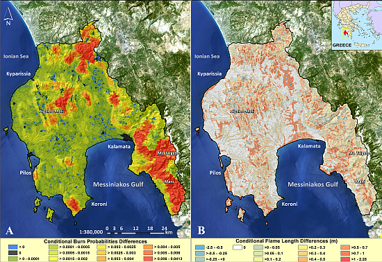
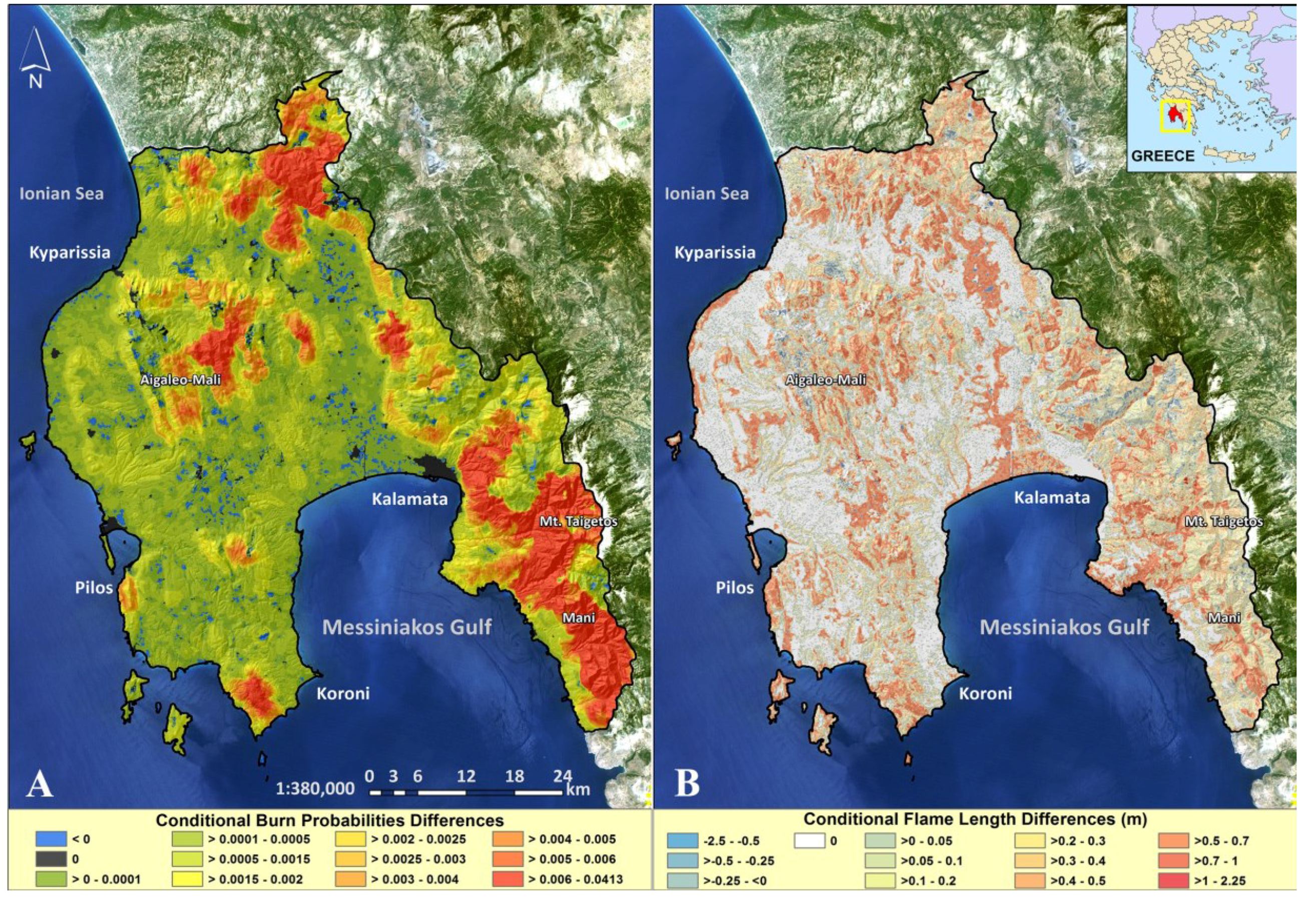
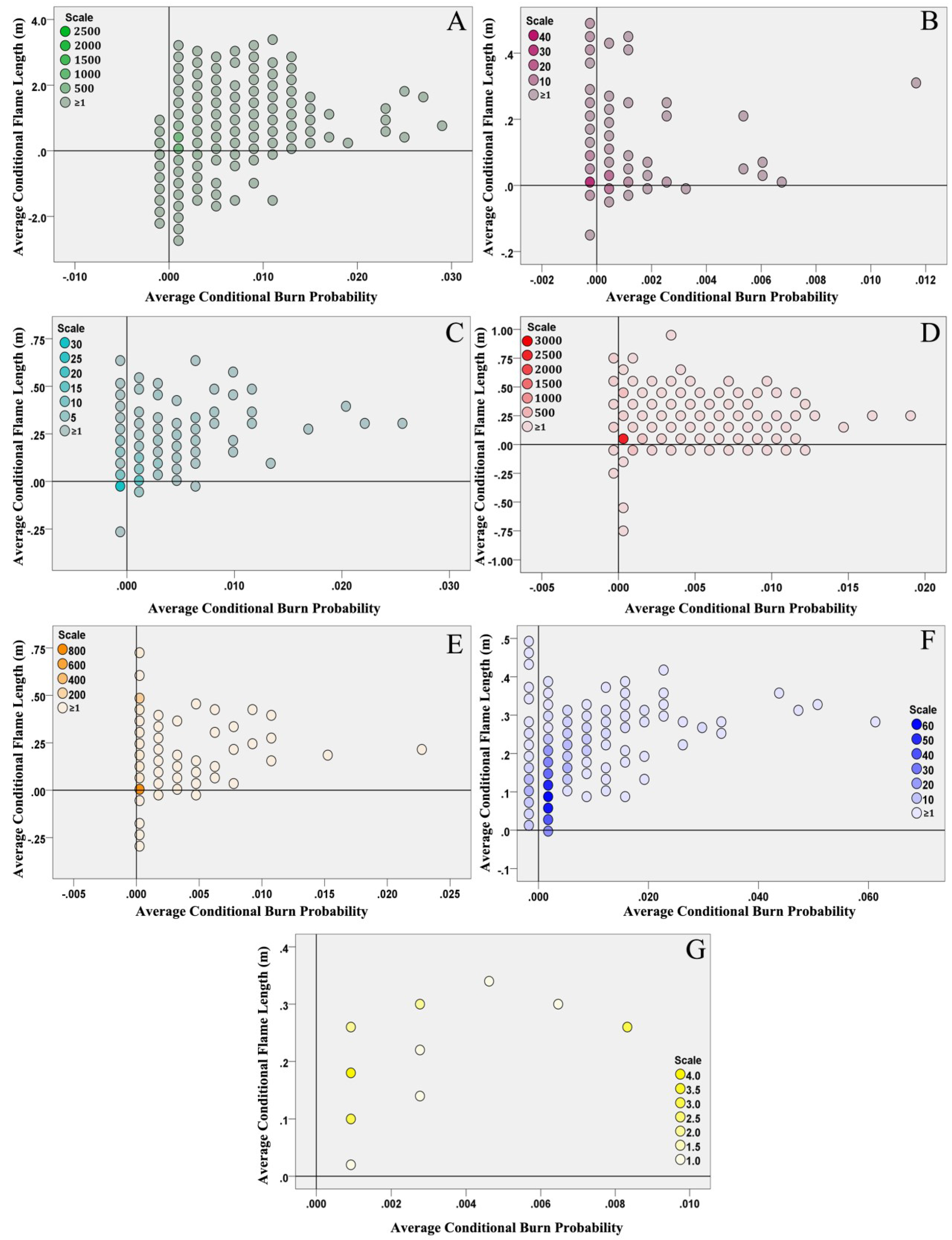
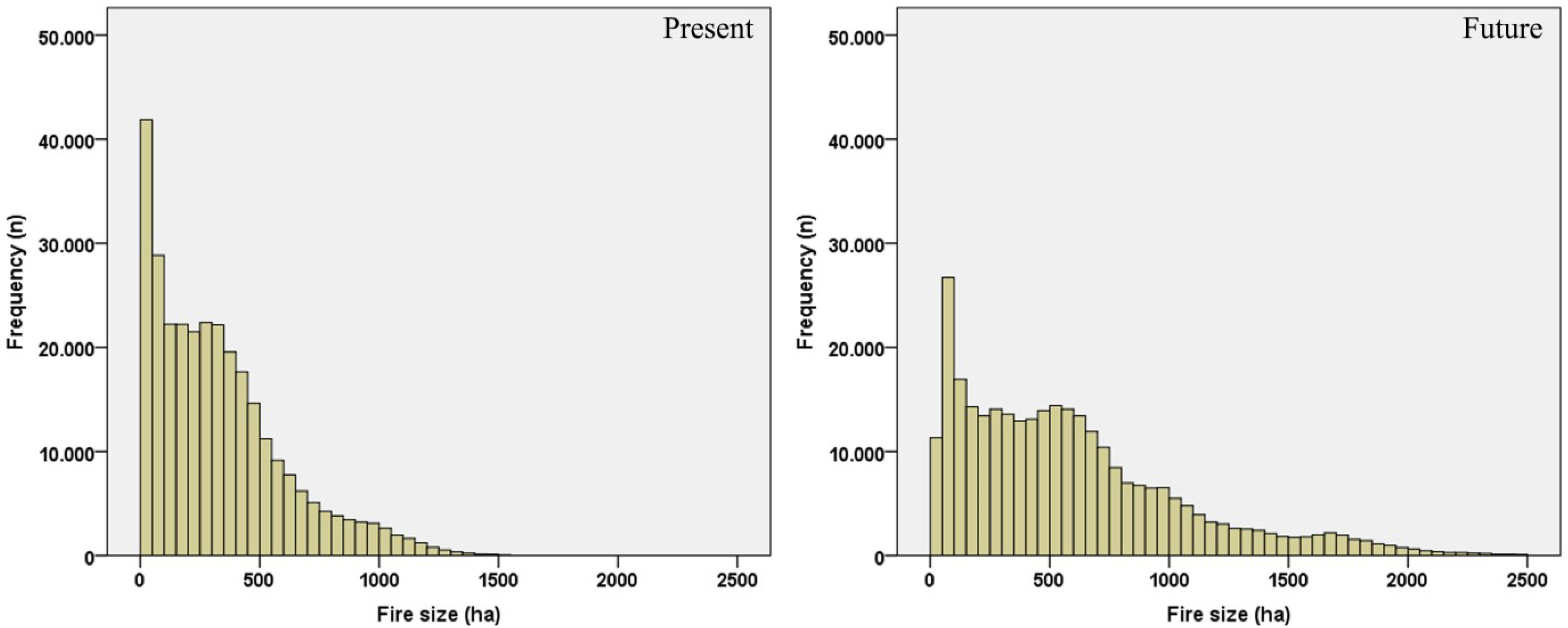
3.2. Randig Simulation Outputs

Randig results for the two time periods produced spatial data for CBP and CFL regarding the three sub-areas of Messinia. It should be acknowledged that the CBP and CFL are conditional given the presence of a fire resistant to initial control. These spatial data were clipped with the initial boundaries of the three areas and then merged to produce a new raster file for the entire study area. Raster values of the CBP and CFL files for the two time periods were subtracted (i.e., future minus present) to produce new raster files of CBP (Figure 5A) and CFL (Figure 5B) differences. Positive values mean that given a set of 100,000 randomly located ignitions on each LCP, the probability of burning given the specified weather scenarios has increased under future climate; while on the contrary, negative values reveal a decrease. Furthermore, a file with the simulated fire ignition points, along with their burned areas (ha), was derived and used to create histograms of fire size vs. frequency (Figure 6). Randig outputs were used for averaging the area around each value-at-risk attribute and then to create scatterplots to estimate the landscape-based conditional likelihood of burning (CBP) and potential intensity (CFL) (Figure 7), highlighting “hot spots” for fuel treatment planning [80].
Figure 5. (A) Conditional burn probability and (B) conditional flame length differences of present and future time periods in Messinia, Greece.
Forests 06 02214 g005
Spatial results revealed that CBP and CFL are projected to increase under future climate change conditions on 93.5% and 62% of the landscape, respectively (Figure 5). A low (greater than 0 to 0.001), moderate (greater than 0.001 to 0.006) and high (greater than 0.006) increase on future CBP values was calculated on 55.8%, 26.8% and 10.7% of the total study area, respectively; with only a 2.65% decrease and 4.05% zero change across the landscape. A low (greater than 0 to 0.2 m), moderate (from 0.2 to 0.5 m) and high (greater than 0.5 m) increase on future CFL values was calculated on 25%, 28% and 9% of the total study area, respectively; a decrease of CFL was calculated on the 2.13% of cells, mostly scattered across the landscape with very few concentrations (from 0 to −0.01 m on 0.47%; from −0.01 to −0.1 m on 1.02%; and less than −0.1 m on 0.64%). Significant parts of the landscape (35.87%) did not have any change on CFL values, located mainly in the coastal zones and plains of Messinia, mostly on fuel models GS1 (75%), GR2 (8%) and SH7 (4%). It is important for the reader to acknowledge that these results must be interpreted as conditional, meaning that under different simulation parameters absolute values can change, and emphasis should be given only at the general trends of spatial change.
The SE tip of the Messinia region (i.e., Mount Taigetos and Mani areas that comprise about 7% of the total study area) is expected to experience a large increase in CBP vs. the present predicted conditions (Figure 5A). The primary vegetation types of the area to carry the wildfires are conifer forests, evergreen shrublands and reforested agricultural areas. An average increase of approximately 0.3 m in the CFL values was estimated for these areas (Figure 5B). Another area with high CBP increase is on the northern part (about 4% of total study area), covered with evergreen shrublands, oak woodlands and reforested agricultural areas (Figure 5A). The area west of Koroni in the south (about 3% of total study area), mainly covered with evergreen shrublands, has also increased CBP values as well as the area of Pilos on the west (Figure 5A), both having a well-developed tourism sector. CFL values in these two last areas are also expected to have a large average increase of approximately 0.5 m (Figure 5B). Large increase in CFL values (>0.5 m) was calculated for the small islands south and west of Messinia (Figure 5B). The area east of the Aigaleo-Mali forest (central part of Messinia) also has increased CBP values for the future time period (Figure 5A). The coastal zone south from Kyparissia has an average increase of CFL values by 0.4 m, covered mainly by agricultural zones (Figure 5B).
A clear trend for increased fire size exists in Figure 6, having higher frequency for fire sizes more than 500 ha. It is expected that the number of small forest fires (<10 ha) will be reduced in favor of larger fires. The present situation produced 30% of fire events greater than 500 ha, while the future situation outputs had about 50%. Fire sizes of 1000 ha were rare for present (almost 5%), and increased to 15% for future conditions. The average burned area per simulated fire (without any simulated suppression effort), is estimated to increase from 334 ha to 589 ha for the future time period, an expected increase of 76%.
Figure 6. Histograms of fire size vs. frequency of present and future time periods.
Forests 06 02214 g006
Figure 7. Hex-binned scatterplots of the two time periods CBP and CFL differences (Future minus Present) for: (A) agricultural installations; (B) hotels, (C) monuments, (D) houses, (E) industries/businesses, (F) WUI sites and (G) wildlife habitats (scale refers to the number of cases contained at each colored hex bin).
Forests 06 02214 g007
Values-at-risk were plotted with hex-binned scatterplots (Figure 7). Agricultural installations have a moderate percentage of attributes that portray increased CBP, while there is a substantial number of installations which portray a decrease in overall average CBP (5%) and CFL values (12%) (Figure 7A). Although most of the hotels seem relatively less vulnerable, with low CBP and CFL increases, extra attention must be given for those few facilities with high expected vulnerability in the future (Figure 7B). A decrease in overall average CBP and CFL values was predicted for 5.5% and 12% of the records, respectively. Half of the monuments across Messinia have the potential of increased vulnerability in the future and require attention and protective measures (Figure 7C). A decrease in overall average CBP and CFL values was predicted for 4.3% and 5% of the records, respectively. Hundreds of houses are also expected to increase their CBP and CFL values, but the vast majority does not portray any change in future vulnerability (Figure 7D). A decrease in overall average CBP and CFL values was predicted for 4.2% and 1.1% of the records, respectively. About 15% of industries and businesses will have CBP and CFL increase, with the rest of the attributes remaining on present time period risk levels (Figure 7E). A decrease in overall average CBP and CFL values was predicted for 8% and 2% of the records, respectively. There is a large number of WUI sites located on currently abandoned cultivated areas that have a substantial increase in CBP values; thus, it is more likely to burn in the future due to larger simulated fire sizes (Figure 7F). The decrease in overall average CBP and CFL values is very low (<1%). Finally, the majority of wildlife habitats was calculated to experience a moderate to small vulnerability change in the future period (Figure 7G), without any record having a decrease at their future values.

4. Conclusions

Climate change research and forest fire science are in a continuous state of evolution and as our understanding of how different aspects of climate interaction is expanding, so does our ability to forecast future wildfire behavior. The main approach of this study was to use state-of-the-art fire behavior models to simulate burn probability, size and intensity of present and future wildfire events that are resistant to control and thus, to estimate the degree of change of each climatic scenario relative to the other. The study has not tried to replicate historic fires, but to project impact to highly valued resources based on large fires resistant to control that burn actively for several hours. Limitations and assumptions are inherently inside each model, and several assumptions were made to transform RCM outputs to fire behavior model inputs. A key assumption is that the CBP and CFL are conditional given the presence of a fire resistant to initial control. Furthermore, scenarios were primarily created based on the wind speed and direction frequencies of the total number of observation days, since wind is the key driving force of wildfire propagation in Messinia. Wind scenarios were linked with relevant temperature and relative humidity to calculate dead FMC values with the derived data, while live FMC values were based on the BehavePlus fuel moisture scenarios with a change to the next driest category for the future time period. Since almost all wildfires in Greece experience some kind of firefighting operations (and Randig modeling is conducted with no suppression simulation), results should be interpreted as the uncontained modeling outputs for present and future time periods. Readers should not place emphasis on the numerical levels of any single aspect of the model’s conditional results in isolation, but rather understand and assess the general patterns predicted by the models.
Analysis of FWI estimated values between the two time periods revealed that a reduction on the number of days with low FWI is expected, in favor of more frequent days with high or extreme FWI values. A positive correlation between wildfire ignitions and FWI values and the ever-increasing human influence on wildfire ignition frequencies indicate that more wildfires are expected in the future period that will definitely affect the wildfire control practices and effectiveness. The number of days with elevated fire risks increases by more than a month between 2071 and 2100, leading to significantly longer fire seasons for the area of Messinia in the future.
Based on the results, large wildfires with increasing size and intensity are expected to occur in the Messinia region towards the end of the 21st century, resulting in increasing conditional burn probabilities across much of the landscape. Fire size is likely to have an increase that can substantially affect values-at-risk. Thousands of wildfire simulations and several tests prior to producing the results of our study provided evidence that the drivers of this increase are chiefly the cumulative effect of decreased fuel moistures, along with increased wind speeds and spotting (used as described in Materials and Methods). RCM-predicted lower relative humidity values are expected to lead to an increase in future ignition frequencies, since fuel moisture has been linked to ignition probability [82]; it is important to note that this study did not account for those possible variations on ignition probability. If future vegetation/fuel conditions could be projected and accounted for in Randig simulations, different intensity levels and conditional burn probabilities are to be expected. By keeping the fuel conditions stable between the two time periods, the main source of stochasticity in the modeling procedure was the random ignition locations and the weather scenario under which the fire subsequently burns. Any calculated change was caused by these two parameters; thus, the decrease on some CBP and CFL pixels values had to do with the differences of wildfire ignitions, wind direction and speed category frequency and live and dead FMC values. It is important to note that those differences were very low and appeared on a very small portion of the study area.
Conditional results of the uncontained fire behavior simulations revealed that numerous houses and agricultural installations will be affected by the upcoming changes in fire behavior due to their dispersed location on the landscape, and owners will have to take extra care and fire prevention measures to protect their property. Although most of the hotels do not portray any vulnerability change, extra attention must be given for those few facilities located on future high CBP and CFL areas. Monuments and cultural heritage sites have a significant shift in their risk values, and by considering that most of them are under a low protection status, they will probably need extra protection to avoid damages or destruction. During the 2007 season wildfires, the area of ancient Olympia (birthplace of the Olympic Games), a world heritage site very close to Messinia, partially burned from raging wildfires causing worldwide distress and a negative impact; and a newer catastrophe of this scale must be avoided at all costs. WUI will probably face larger and more intense fires during the future period and as more people tend to reside in these areas (suburbs), the risk to property and human lives will increase. Installations of industrial infrastructure on the RUI, such as solar panels and greenhouses, have high risk; and to avoid economic loses, owners must create fire protection zones around them. It is expected that wildlife habitats will also experience more intense and larger fires, thus prioritization of areas requiring the most attention must be made in advance. A decrease in future minus present average CBP and CFL values was calculated for most values-at-risk on a considerable amount of records. This has to do with the small number of pixels that has a lower value in the future compared to present time period modeling results (approximately 2%). It is important to note that most of these differences were insignificant, with very small values.
Since weather patterns cannot be changed or modified directly by humans on a local or regional scale and during the time needed (weather hypothesis), the only option left for protecting societies and values-at-risk is by modifying vegetation and fuel patterns (fuel hypothesis) in an effort to reduce fuel availability and control at some point of the wildfire activity. As a result, fuel reduction activities will likely continue to grow over time in response to the changing climate and the concomitant increase in fuel loads and fire [83,84,85]. This study’s outcomes emphasize the need for fuel treatment techniques aiming at reducing vegetation fuel accumulations, strategically implemented around areas and facilities that have high hazard and vulnerability.
Landscape fuel treatment plans can be derived from a number of methods, including the use of models such as the Treatment Optimization Model (TOM) within FlamMap [59] or the Landscape Treatment Designer (LTD) within ArcFuels10 [80], based on specific needs (point protection of structures), wildfire risks, or expert opinion. Implementation of similar procedures as those used during this research can be applied and tested prior to any treatment of vegetation modification in the fields, in order to conclude which treatments are the most appropriate for each area of interest.

Acknowledgments

The study was supported by XENIOS project (no. 09COP-31-867), financed by the EU (ERDF) and Greek national funds through the Operational Program “Competitiveness and Entrepreneurship” of the National Strategic Reference Framework (NSRF) Research Funding Program COOPERATION 2009, and the Academy of Athens. The authors would like to thank the Navarino Environmental Observatory (NEO) for its support in data collection. Alan Ager and Mark Finney, Research Scientists of the United States Department of Agriculture, are acknowledged for providing valuable scientific contributions relevant to their cited work in this research. Anonymous peer reviewers must also be thanked for their efforts to offer very useful comments in earlier versions of the manuscript.

Conflicts of Interest

The authors declare no conflict of interest.

References

  1. Intergovernmental Panel on Climate Change (IPCC). Climate Change 2007: The physical science basis. In Contribution of Working Group I to the Intergovernmental Panel on Climate Change, Fourth Assessment Report; Solomon, S., Qin, D., Manning, M., Chen, Z., Marquis, M., Averyt, K.B., Tignor, M., Miller, H.L., Eds.; Cambridge University Press: Cambridge, UK; New York, NY, USA, 2007; pp. 1–996. [Google Scholar]
  2. Flannigan, M.D.; Logan, K.A.; Amiro, B.D.; Skinner, W.R.; Stocks, B.J. Future area burned in Canada. Clim. Chang. 2005, 72, 1–16. [Google Scholar] [CrossRef]
  3. Intergovernmental Panel on Climate Change (IPCC). Climate Change 2007: Impacts, Adaptation and Vulnerability. In Contribution of Working Group II to the Intergovernmental Panel on Climate Change, Fourth Assessment Report; Solomon, S., Qin, D., Manning, M., Chen, Z., Marquis, M., Averyt, K.B., Tignor, M., Miller, H.L., Eds.; Cambridge University Press: Cambridge, UK; New York, NY, USA, 2007; pp. 1–22. [Google Scholar]
  4. Stocks, B.J.; Fosberg, M.A.; Lynham, T.J.; Mearns, L.; Wotton, B.M.; Yang, Q.; Jin, J.Z.; Lawrence, K.; Hartley, G.R.; Mason, J.A.; et al. Climate change and forest fire potential in Russian and Canadian boreal forests. Clim. Chang. 1998, 38, 1–13. [Google Scholar] [CrossRef]
  5. Flannigan, M.D.; Stocks, B.J.; Wotton, B.M. Climate change and forest fires. Sci. Total Environ. 2000, 262, 221–229. [Google Scholar] [CrossRef]
  6. Fried, J.S.; Torn, M.S.; Mills, E. The impact of climate change on wildfire severity: A regional forecast for northern California. Clim. Chang. 2004, 64, 169–191. [Google Scholar] [CrossRef]
  7. Mouillot, F.; Rambal, S.; Joffre, R. Simulating climate change impacts on fire frequency and vegetation dynamics in a Mediterranean type ecosystem. Glob. Chang. Biol. 2002, 8, 423–437. [Google Scholar] [CrossRef]
  8. Scheffer, M.; Carpenter, S.; Foley, J.; Folke, C.; Walker, B. Catastrophic shifts in ecosystems. Nature 2001, 413, 591–596. [Google Scholar] [CrossRef] [PubMed]
  9. North, M.; Hurteau, M.; Innes, J. Fire suppression and fuels treatment effects on mixed conifer carbon stocks and emissions. Ecol. Appl. 2009, 19, 1385–1396. [Google Scholar] [CrossRef] [PubMed]
  10. Stephens, S.L.; Moghaddas, J.J.; Hartsouogh, B.R.; Moghaddas, E.E.Y.; Clinton, N.E. Fuel treatment effects on stand level carbon pools, treatment related emissions, and fire risk in a Sierra Nevada mixed conifer forest. Can. J. For. Res. 2009, 39, 1538–1547. [Google Scholar] [CrossRef]
  11. Weidinmyer, C.; Hurteau, M.D. Prescribed fire as a means of reducing forest carbon emissions in the western United States. Environ. Sci. Technol. 2010, 44, 1926–1932. [Google Scholar] [CrossRef] [PubMed]
  12. Intergovernmental Panel on Climate Change (IPCC). Climate Change 2013: The Physical Science Basis. In Contribution of Working Group I to the Intergovernmental Panel on Climate Change, Fifth Assessment Report; Stocker, T.F., Qin, D., Plattner, G.K., Tignor, M., Allen, S.K., Boschung, J., Nauels, A., Xia, Y., Bex, V., Midgley, P.M., Eds.; Cambridge University Press: Cambridge, UK; New York, NY, USA, 2013; pp. 1–1535. [Google Scholar]
  13. Lionello, P. The Climate of the Mediterranean Region: From the Past to the Future; Elsevier Inc.: Amsterdam, The Netherlands, 2012. [Google Scholar]
  14. Climate Change Impacts Study Committee. The Environmental, Economic, and Social Impacts of Climate Change in Greece; Bank of Greece: Athens, Greece, 2011; pp. 1–494. Available online: http://www.bankofgreece.gr/BoGEkdoseis/ClimateChange_FullReport_bm.pdf (accessed on 1 June 2015).
  15. Giorgi, F.; Lionello, P. Climate change projections for the Mediterranean region. Glob. Planet. Chang. 2008, 63, 90–104. [Google Scholar] [CrossRef]
  16. Sheffield, J.; Wood, E.F. Projected changes in drought occurrence under future global warming from multi-model, multi scenario, IPCC AR4 simulations. Clim. Dyn. 2008, 31, 79–105. [Google Scholar] [CrossRef]
  17. Giannakopoulos, C.; Le Sager, P.; Bindi, M.; Moriondo, M.; Kostopoulou, E.; Goodess, C.M. Climatic changes and associated impacts in the Mediterranean resulting from a 2 °C global warming. Glob. Planet. Chang. 2009, 68, 209–224. [Google Scholar] [CrossRef]
  18. Kioutsioukis, I.; Melas, D.; Zerefos, C. Statistical assessment of changes in climate extremes over Greece (1955–2002). Int. J. Climatol. 2010, 30, 1723–1737. [Google Scholar] [CrossRef]
  19. Kostopoulou, E.; Giannakopoulos, C.; Hatzaki, M.; Tziotziou, K. Climate extremes in the NE Mediterranean: Assessing the E-OBS dataset and regional climate simulations. Clim. Res. 2012, 54, 249–270. [Google Scholar] [CrossRef]
  20. Kostopoulou, E.; Jones, P.D. Assessment of climate extremes in the Eastern Mediterranean. Meteor. Atmos. Phys. 2005, 89, 69–85. [Google Scholar] [CrossRef]
  21. Kuglitsch, F.G.; Toreti, A.; Xoplaki, E.; Della-Marta, P.M.; Zerefos, C.S.; Türkeş, M.; Luterbacher, J. Heat wave changes in the eastern Mediterranean since 1960. Geophys. Res. Lett. 2010, 37, L04802. Available online: http://onlinelibrary.wiley.com/enhanced/exportCitation/doi/10.1029/2009GL041841 (accessed on 21 January 2015). [Google Scholar] [CrossRef]
  22. Giannakopoulos, C.; Kostopoulou, E.; Varotsos, K.V.; Tziotziou, K.; Plitharas, A. An integrated assessment of climate change impacts for Greece in the near future. Reg. Environ. Chang. 2011, 11, 829–843. [Google Scholar] [CrossRef]
  23. Founda, D.; Giannakopoulos, C. The exceptionally hot summer of 2007 in Athens, Greece—A typical summer in the future climate? Glob. Planet. Chang. 2009, 67, 227–236. [Google Scholar] [CrossRef]
  24. Trigo, R.M.; Pereira, J.; Pereira, M.G.; Mota, B.; Calado, T.J.; Dacamara, C.C.; Santo, F.E. Atmospheric conditions associated with the exceptional fire season of 2003 in Portugal. Int. J. Climatol. 2006, 26, 1741–1757. [Google Scholar] [CrossRef]
  25. Koutsias, N.; Arianoutsou, M.; Kallimanis, A.S.; Mallinis, G.; Halley, J.M.; Dimopoulos, P. Where did the fires burn in Peloponnisos, Greece the summer of 2007? Evidence for a synergy of fuel and weather. Agric. For. Meteor. 2012, 156, 41–53. [Google Scholar] [CrossRef]
  26. EFFIS. Forest Fires in Europe; Report No 8, JRC Scientific and Technical Reports. Available online: http://forest.jrc.ec.europa.eu/media/cms_page_media/9/01-forest-fires-in-europe-2007.pdf (accessed on 1 June 2015).
  27. Koutsias, N.; Xanthopoulos, G.; Founda, D.; Xystrakis, F.; Nioti, F.; Pleniou, M.; Mallinis, G.; Arianoutsou, M. On the relationships between forest fires and weather conditions in Greece from long-term national observations (1894–2010). Int. J. Wildland Fire 2012, 22, 493–507. [Google Scholar] [CrossRef]
  28. Moreira, F.; Arianoutsou, M.; Corona, P.; de las Heras, J. Post-Fire Management and Restoration of Southern European Forests; Springer Dordrecht Heidelberg: London, UK; New York, NY, USA, 2012. [Google Scholar]
  29. Bessie, W.C.; Johnson, E.A. The relative importance of fuels and weather on fire behavior in subalpine forests. Ecology 1995, 76, 747–762. [Google Scholar] [CrossRef]
  30. Agee, J.K. The severe weather wildfire—Too hot to handle? Northwest. Sci. 1997, 71, 153–156. [Google Scholar]
  31. Keeley, J.E.; Fotheringham, C.J. History and management of crown-fire ecosystems: A summary and response. Conserv. Biol. 2001, 15, 1561–1567. [Google Scholar] [CrossRef]
  32. Van Wagner, C.E. Development and structure of the Canadian Forest Fire Weather Index System. In Forestry Technical Report 35; Canadian Forestry Service: Ottawa, ON, Canada, 1987; pp. 1–37. [Google Scholar]
  33. Stocks, B.J.; Lawson, B.D.; Alexander, M.E.; van Wagner, C.E.; McAlpine, R.S.; Lynham, T.J.; Dube, D.E. The Canadian Forest Fire Danger Rating System: An Overview. For. Chron. 1989, 65, 450–457. [Google Scholar] [CrossRef]
  34. Baltas, E.A. Climatic conditions and availability of water resources in Greece. Int. J. Water Resour. D 2008, 24, 635–649. [Google Scholar] [CrossRef]
  35. Klein, J.; K. Ekstedt, K.; Walter, M.T.; Lyon, S.W. Modeling potential water resource impacts of Mediterranean tourism in a changing climate. Environ. Model. Assess. 2015, 20, 117–128. [Google Scholar] [CrossRef]
  36. Flocas, A.A. Frontal depressions over the Mediterranean Sea and central southern Europe. (Les perturbations frontales au-dessus de la mer Méditerranée et de l' Europe centrale méridionale). Mediterranee 1988, 66, 43–52. (In French) [Google Scholar] [CrossRef]
  37. Trigo, I.F.; Grant, R.B.; Trevor, D.D. Climatology of Cyclogenesis Mechanisms in the Mediterranean. Mon. Weather Rev. 2002, 130, 549–569. [Google Scholar] [CrossRef]
  38. Hellenic Fire Service. Available online: http://www.fireservice.gr/pyr/site/home.csp (accessed on 1 June 2015).
  39. Mazarakis, N.; Kotroni, V.; Lagouvardos, K.; Argiriou, A.A. Storms and lightning activity in Greece during the warm periods of 2003–06. J. Appl. Meteorol. Clim. 2008, 47, 3089–3098. [Google Scholar] [CrossRef]
  40. Defer, E.; Lagouvardos, K.; Kotroni, V. Lightning activity in the eastern Mediterranean region. J. Geophys. Res. 2005, 110, D24210. [Google Scholar] [CrossRef]
  41. Lenderink, G.; van den Hurk, B.; van Meijgaard, E.; van Ulden, A.P.; Cuijpers, J.H. Simulation of Present-Day Climate in RACMO2: First Results and Model Developments. KNMI Technical Report, 252; Koninklijk Nederlands Meteorologisch Instituut: Amsterdam, The Netherlands, 2003. [Google Scholar]
  42. Lenderink, G.; van Ulden, A.; van den Hurk, B.; Keller, F. A study on combining global and regional climate model results for generating climate scenarios of temperature and precipitation for the Netherlands. Clim. Dyn. 2007, 29, 157–176. [Google Scholar] [CrossRef]
  43. Van Ulft, L.H.; van de Berg, W.J.; Bosveld, F.C.; van den Hurk, B.J.J.M.; Lenderink, G.; Siebesma, A.P. The KNMI Regional Atmospheric Climate Model RACMO Version 2.1; Technical Repost TR-302; KNMI: De Bilt, The Netherlands, 2008; pp. 1–43. [Google Scholar]
  44. Tank, A.; Beersma, J.; Bessembinder, J.; van den Hurk, B.; Lenderink, G. KNMI’14 Climate Scenarios for the Netherlands, A Guide for Professionals in Climate Adaptation; KNMI: De Bilt, The Netherlands, 2014; pp. 1–34. [Google Scholar]
  45. Nakicenovic, N.; Alcamo, J.; Davis, G.; de Vries, B.; Fenhann, J.; Gaffin, S.; Gregory, K.; Grübler, A.; Jung, T.Y.; Kram, T.; et al. Emission scenarios. In A Special Report of Working Group III of the Intergovernmental Panel on Climate Change; Cambridge University Press: Cambridge, UK; New York, NY, USA, 2000. [Google Scholar]
  46. ENSEMBLES Deliverable D3.2.2: RCM-Specific Weights Based on Their Ability to Simulate the Present Climate, Calibrated for the ERA40-Based Simulations. Available online: http://ensembles-eu.metoffice.com/deliverables.html (accessed on 1 June 2015).
  47. Christensen, J.H.; Kjellström, E.; Giorgi, F.; Lenderink, G.; Rummukainen, M. Weight assignment in regional climate models. Clim. Res. 2010, 44, 179–194. [Google Scholar] [CrossRef]
  48. Lawson, B.D.; Armitage, O.B. Weather guide for the Canadian Forest Fire Danger Rating System. Natural Resources Canada, Canadian Forest Service: Edmonton, AB, Canada, 2008; pp. 1–73. Available online: http://cfs.nrcan.gc.ca/pubwarehouse/pdfs/29152.pdf (accessed on 1 June 2015).
  49. Viegas, D.X.; Bovio, G.; Ferreira, A.; Nosenzo, A.; Bernard, S. Comparative study of various methods of fire danger evaluation in Southern Europe. Int. J. Wildland Fire 1999, 9, 235–246. [Google Scholar] [CrossRef]
  50. Moriondo, M.; Good, P.; Durao, R.; Bindi, M.; Giannakopoulos, C.; Corte-Real, J. Potential impact of climate change on fire risk in the Mediterranean area. Clim. Res. 2006, 31, 85–95. [Google Scholar] [CrossRef]
  51. Carvalho, A.; Flannigan, M.D.; Logan, K.; Miranda, A.I.; Borrego, C. Fire activity in Portugal and its relationship to weather and the Canadian Fire Weather Index System. Int. J. Wildland Fire 2008, 17, 328–338. [Google Scholar] [CrossRef]
  52. Good, P.; Moriondo, M.; Giannakopoulos, C.; Bindi, M. The meteorological conditions associated with extreme fire risk in Italy and Greece: Relevance to climate model studies. Int. J. Wildland Fire 2008, 17, 155–165. [Google Scholar] [CrossRef]
  53. Dimitrakopoulos, A.P.; Bemmerzouk, A.M.; Mitsopoulos, I.D. Evaluation of the Canadian fire weather index system in an eastern Mediterranean environment. Meteorol. Appl. 2011, 18, 83–93. [Google Scholar] [CrossRef]
  54. Giannakopoulos, C.; LeSager, P.; Moriondo, M.; Bindi, M.; Karali, A.; Hatzaki, M.; Kostopoulou, E. Comparison of fire danger indices in the Mediterranean for present day conditions. iForest 2012, 5, 197–203. [Google Scholar] [CrossRef]
  55. Karali, A.; Hatzaki, M.; Giannakopoulos, C.; Roussos, A.; Xanthopoulos, G.; Tenentes, V. Sensitivity and evaluation of current fire risk and future projections due to climate change: The case study of Greece. Nat. Hazard. Earth Syst. 2014, 14, 143–153. [Google Scholar] [CrossRef] [Green Version]
  56. Finney, M.A. Fire growth using minimum travel time methods. Can. J. For. Res. 2002, 32, 1420–1424. [Google Scholar] [CrossRef]
  57. Finney, M.A. A Computational Method for Optimizing Fuel Treatment Locations. In Rocky Mountain Research Station Proceedings RMRS-P-41, Proceedings of the Fuels Management—How to Measure Success, Portland, OR, USA, 27–30 March 2006; Andrews, P.L., Butler, B.W., Eds.; USDA Forest Service: Fort Collins, CO, USA, 2006; pp. 107–124. [Google Scholar]
  58. Finney, M.A. An overview of FlamMap fire modeling capabilities. In Rocky Mountain Research Station Proceedings RMRS-P-41, Proceedings of the Fuels Management—How to Measure Success, Portland, OR, USA, 27–30 March 2006; Andrews, P.L., Butler, B.W., Eds.; USDA Forest Service: Fort Collins, CO, USA, 2006; pp. 213–220. [Google Scholar]
  59. Richards, G.D. An elliptical growth model of forest fire fronts and its numerical solutions. Int. J. Numer. Meth. Eng. 1990, 30, 1163–1179. [Google Scholar] [CrossRef]
  60. Ager, A.A.; Vaillant, N.M.; Finney, M.A.; Preisler, H.K. Analyzing wildfire exposure and source–sink relationships on a fire prone forest landscape. For. Ecol. Manag. 2012, 267, 271–283. [Google Scholar] [CrossRef]
  61. Byram, G.M. Combustion of forest fuels. In Forest Fire: Control and Use; Davis, K.P., Ed.; McGraw-Hill: New York, NY, USA, 1959; pp. 61–89. [Google Scholar]
  62. Catchpole, E.A.; de Mestre, N.J.; Gill, A.M. Intensity of fire at its perimeter. Aust. For. Res. 1982, 12, 47–54. [Google Scholar]
  63. Ager, A.A.; Vaillant, N. A comparison of landscape fuel treatment strategies to mitigate wildland fire risk in the urban interface and preserve old forest structure. For. Ecol. Manag. 2010, 259, 1556–1570. [Google Scholar] [CrossRef]
  64. Finney, M.A. FARSITE: Fire Area Simulator—Model Development and Evaluation; Research Paper RMRS-RP-4; USDA Forest Service, Rocky Mountain Research Station: Ogden, UT, USA, 1998; pp. 1–47. [Google Scholar]
  65. Scott, J.H.; Burgan, R.E. Standard Fire Behavior Fuel Models: A Comprehensive Set for Use with Rothermel’s Surface Fire Spread Model; General Technical Report RMRS-GTR-153; USDA Forest Service, Rocky Mountain Research Station: Fort Collins, CO, USA, 2005. [Google Scholar]
  66. Palaiologou, P.; Kalabokidis, K.; Kyriakidis, P. Forest mapping by geoinformatics for landscape fire behaviour modelling in coastal forests, Greece. Int. J. Remote Sens. 2013, 34, 4466–4490. [Google Scholar] [CrossRef]
  67. Dimitrakopoulos, A.P.; Panov, P.I. Pyric properties of some dominant Mediterranean vegetation species. Int. J. Wildland Fire 2001, 10, 23–27. [Google Scholar] [CrossRef]
  68. Brown, J.K. Weight and Density of Crowns of Rocky Mountain Conifers; Research Paper INT-197; USDA Forest Service, Intermountain Forest and Range Experiment Station: Ogden, UT, USA, 1978; pp. 1–56. [Google Scholar]
  69. Keane, R.E.; Mincemoyer, S.A.; Schmidt, K.M.; Long, D.G.; Garner, J.L. Mapping Vegetation and Fuels for Fire Management on the Gila National Forest Complex, New Mexico, [CD-ROM]. General Technical Report RMRS-GTR-46-CD; USDA Forest Service, Rocky Mountain Research Station: Ogden, UT, USA, 2000; pp. 1–126. [Google Scholar]
  70. Scott, J.H.; Reinhardt, E.D. Estimating canopy fuels in conifer forests. Fire Manag. Today 2002, 62, 45–50. [Google Scholar]
  71. Cruz, M.G.; Alexander, M.E.; Wakimoto, R.H. Assessing canopy fuel stratum characteristics in crown fire prone fuel types of western North America. Int. J. Wildland Fire 2003, 12, 39–50. [Google Scholar] [CrossRef]
  72. Scott, J.H.; Reinhardt, E.D. Stereo Photo Guide for Estimating Canopy Fuel Characteristics in Conifer Stands; General Technical Report RMRS-GTR-145; USDA Forest Service, Rocky Mountain Research Station: Fort Collins, CO, USA, 2005; pp. 1–49. [Google Scholar]
  73. Heinsch, F.A.; Andrews, P.L. BehavePlus Fire Modeling System, Version 5.0: Design and Features; General Technical Report RMRS-GTR-249; USDA Forest Service, Rocky Mountain Research Station: Fort Collins, CO, USA, 2010; pp. 1–111. [Google Scholar]
  74. Rothermel, R.C. How to Predict the Spread and Intensity of Forest and Range Fires. General Technical Report INT-143; USDA Forest Service, Intermountain Forest and Range Experiment Station: Ogden, UT, USA, 1983; pp. 1–161. [Google Scholar]
  75. Ager, A.A.; Finney, M.A.; McMahan, A.; Cathcart, J. Measuring the effect of fuel treatments on forest carbon using landscape risk analysis. Nat. Hazard. Earth Syst. 2010, 10, 2515–2526. [Google Scholar] [CrossRef] [Green Version]
  76. Kalabokidis, K.; Palaiologou, P.; Finney, M. Fire Behavior Simulation in Mediterranean Forests Using the Minimum Travel Time Algorithm. In Proceedings of the 4th Fire Behavior and Fuels Conference; Wade, D.D., Fox, R.L., Eds.; International Association of Wildland Fire: Missoula, MT, USA, 2014; pp. 468–492. [Google Scholar]
  77. Scott, J.H.; Reinhardt, E.D. Assessing Crown Fire Potential by Linking Models of Surface and Crown Fire Behavior; Research Paper RMRS-RP-29; USDA Forest Service, Rocky Mountain Research Station: Fort Collins, CO, USA, 2001; pp. 1–59. [Google Scholar]
  78. Forthofer, J.M. Modeling wind in Complex Terrain for Use in Fire Spread Prediction. Master’s Thesis, Colorado State University, Fort Collins, CO, USA, 2007. [Google Scholar]
  79. ESRI. ArcGIS Desktop: Release 10; Environmental Systems Research Institute: Redlands, CA, USA, 2010.
  80. Vaillant, N.M.; Ager, A.A.; Anderson, J. ArcFuels10 System Overview. General Technical Report PNW-GTR-875; USDA Forest Service, Pacific Northwest Research Station: Portland, OR, USA, 2013; pp. 1–65. [Google Scholar]
  81. Kornbrot, D. Point Biserial Correlation. 2014. Available online: http://onlinelibrary.wiley.com/doi/10.1002/9781118445112.stat06227/full (accessed on 1 June 2015).
  82. Andrews, P.L.; Loftsgaarden, D.O.; Bradshaw, L.S. Evaluation of fire danger rating indexes using logistic regression and percentile analysis. Int. J. Wildland Fire 2003, 12, 213–226. [Google Scholar] [CrossRef]
  83. McKenzie, D.; Gedalof, Z.E.; Peterson, D.L.; Mote, P. Climatic change, wildfire, and conservation. Conserv. Biol. 2004, 18, 890–902. [Google Scholar] [CrossRef]
  84. Bachelet, D.; Neilson, R.P.; Lenihan, J.M.; Drapek, R.J. Climate change effects on vegetation distribution and carbon budget in the United States. Ecosystems 2001, 4, 164–185. [Google Scholar] [CrossRef]
  85. Gedalof, Z.; Peterson, D.L.; Mantua, N.J. Atmospheric, climatic, and ecological controls on extreme wildfire years in the northwestern United States. Ecol. Appl. 2005, 15, 154–174. [Google Scholar] [CrossRef]

