2.1. Overview
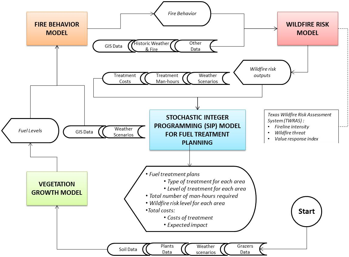
The proposed SIP approach for fuel treatment planning integrates
vegetation growth,
fire behavior, and
wildfire risk as depicted in
Figure 1. The fuel treatment options include
no treatment,
prescribed fire,
mechanical thinning and
grazing. Vegetation growth is modeled using a plant growth modeling software such as the Phytomas Growth Model (PHYGROW) [
17] while fire behavior is modeled using a fire behavior software such as FARSITE [
18]. A wildfire risk model such as the Texas Wildfire Risk Assessment System (TWRAS) [
19] is used to compute wildfire risk parameters of interest, which become inputs to the two-stage SIP model for optimizing fuel treatment plans. The two-stage SIP model determines the fuel treatment plan under uncertainty in fuel levels, weather, and wildfire risk. The fuel levels at any given time can be estimated using a vegetation growth model, for example, while wildfire risk is estimated based on weather and fire behavior. Given the appropriate input data, the SIP model optimizes the here-and-now fuel treatment cost in the first-stage and the expected future costs in the second-stage, which account for the impact of the fuel treatment options selected in the first-stage. Thus the fuel treatment plan specifies the optimal type of fuel treatment for area.
Figure 1.
Schematic diagram of the stochastic integer programming (SIP) methodology.
Figure 1.
Schematic diagram of the stochastic integer programming (SIP) methodology.
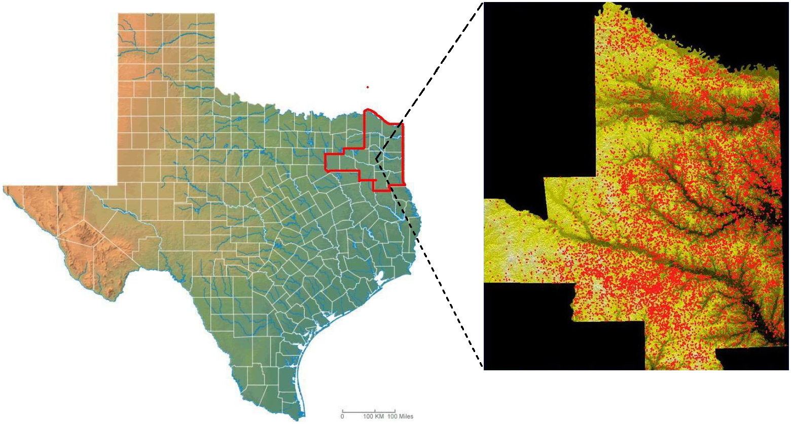
2.2. Study Area
The SIP model was applied to a study area called Texas District 12 (TX12) located in East Texas, USA (
Figure 2), which is under the jurisdiction of Texas A&M Forest Service (TFS). The historical fire data for TX12 shows a total of 13,163 fire occurrences in the period 1985–2006 [
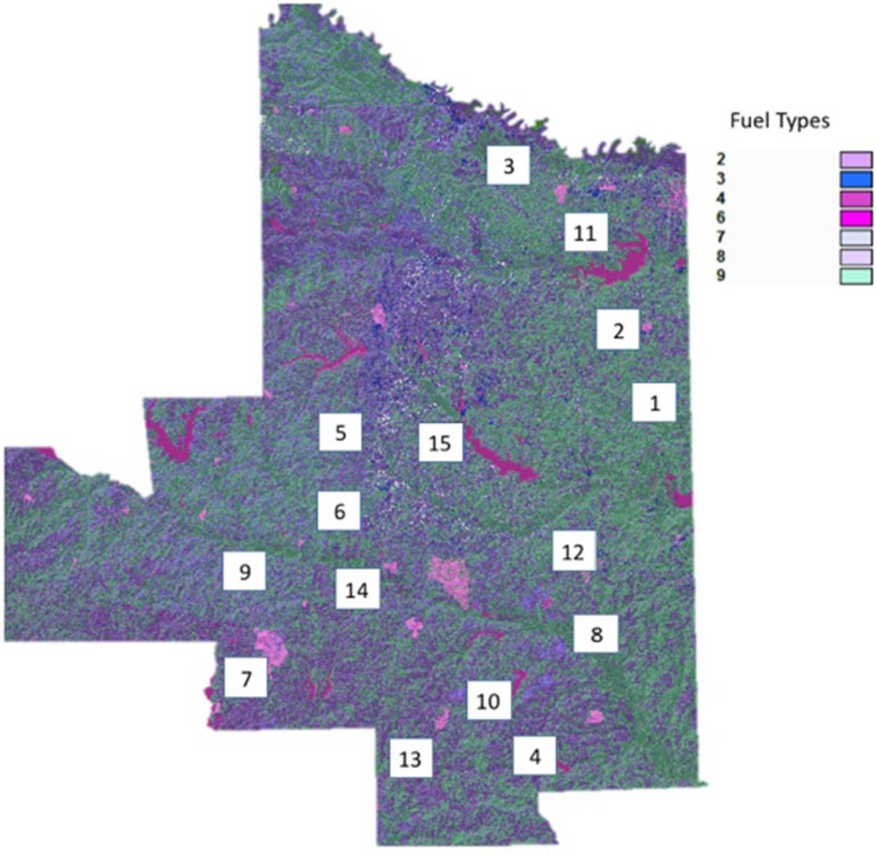
20]. Clearly TX12 is susceptible to wildfires and certain areas of this region can benefit from fuel treatment. To perform our study, 15 areas for fuel treatment (
Figure 3) were selected. These areas had similar vegetation of grass and shrubs and each was arbitrarily set to be about 200 hectares (ha). The areas were chosen with enough distance among them so that they are isolated to prevent any interactions in terms of fire spread. The vegetation growth, fire behavior, and wildfire risk models generate the estimated parameters for the SIP model. However, these models require several field data. Particularly, data describing the landscape, scenario weather, soils, and plants are needed. The data that were available at the time of the study were supplied by the TFS. The type of vegetation in TX12 area includes Northern Forest Fire Laboratory (NFFL) [
21] fuel models 2, 3, 4, 6, 7, 8 and 9.
Table 1 defines each of these fuel models [
21], and
Table 2 shows the dominant fuel models in each area.
Figure 2.
Location of Texas District 12 (TX12) in East Texas [
22] and historical fire occurrences, where each dot represent a fire occurrence.
Figure 2.
Location of Texas District 12 (TX12) in East Texas [
22] and historical fire occurrences, where each dot represent a fire occurrence.
Figure 3.
Selected potential areas for fuel treatment.
Figure 3.
Selected potential areas for fuel treatment.
Table 1.
Fuel models description.
Table 1.
Fuel models description.
| Fuel Model | Typical Fuel Complex | Fuel Loadings |
|---|
| Fuel 1-Hr | Fuel 10-Hr | Fuel 100-Hr |
|---|
| 2 | Timber (grass and understory) | 2 | 1 | 0.5 |
| 3 | Tall grass (2.5 feet) | 3.01 | 0 | 0 |
| 4 | Chaparral | 5.01 | 4.01 | 2 |
| 6 | Dormant brush, hardwood slash | 1.5 | 2.5 | 2 |
| 7 | Southern rough | 1.13 | 1.87 | 1.5 |
| 8 | Closed timber litter | 1.5 | 1 | 2.5 |
| 9 | Hardwood litter | 2.92 | 0.41 | 0.15 |
2.3. SIP Model Description
The goal of the two-stage SIP fuel treatment model is to reduce the here-and-now costs of implementing fuel treatment for a set of selected areas and the expected impact of wildfire measured in dollars. Four fuel treatment options are considered: no treatment (NT), prescribed fire (PF), mechanical treatment (MT), and grazing (G). The no treatment option is assigned to an area if that area cannot be treated because it is not beneficial to do so based on values at risk or if there is other areas that have more priority (e.g., have higher values at risk and fuel levels), or due to budgetary and labor constraints. In the SIP model, the study area is divided into a set of areas to be treated and each area is subdivided into cells of the same size with similar vegetation type and landscape conditions. Each area is a candidate for all or a subset of fuel treatment options depending on what is appropriate for the area. Then the type of fuel treatment is determined by the SIP model under budgetary and labor constraints. The percentage reduction levels for grazing and mechanical treatment are assumed to be 20 or 35 percent. Also, it is assumed that prescribed fire eliminates all undesired fuels in a given cell. The fuel or vegetation levels for each scenario are assumed to be known at the beginning of the fire season. This is done through field studies and GIS data. These fuel levels are configured into the fire behavior simulation, which is then used to simulate the burn of each cell to record the final fire perimeter, fire area, fireline intensity and heat content. These outputs are used along with other measures to determine the wildfire risk rating for each cell. We also allow for the option of using a vegetation growth model such as PHYGROW to estimate the fuel levels at a given point in time. PHYGROW simulates the growth of understory vegetation under different scenarios to account for the uncertainty of weather and soil conditions.
Table 2.
Dominant fuel models in each area.
Table 2.
Dominant fuel models in each area.
| Area Number | First Dominant Fuel | Second Dominant Fuel |
|---|
| 1 | 9 | - |
| 2 | 2 | 9 |
| 3 | 9 | 2 |
| 4 | 9 | 2 |
| 5 | 8 | 2 |
| 6 | 8 | 2 |
| 7 | 2 | - |
| 8 | 9 | 2 |
| 9 | 8 | 9, 2 |
| 10 | 9 | 2 |
| 11 | 9 | 3, 2 |
| 12 | 9 | 2 |
| 13 | 2 | - |
| 14 | 9 | 2 |
| 15 | 9 | 8, 2 |
The objective of the SIP model is to minimize the total costs of fuel treatment and the expected impact from potential fires based on the fuel treatment carried out. The fuel treatment costs in the model include direct labor and the cost of equipment. The impact from potential wildfires is the values-at-risk includes endangered species losses, carbon emissions, and soil erosion. We refer to this as the ecosystem services provided by the rural forests in terms of dollars. To mathematically state the SIP model, we first describe our notation and then give the formulation.
Sets
Set of all scenarios (based on weather conditions, fuel loadings)
Index set for fuel treatment types
Index set for treatment areas
First-Stage Decision Variables First-Stage Parameters:
dij—Number of man-days necessary to do fuel treatment
at area
D—Total number of man-days available for performing fuel treatments
cij—Cost of fuel treatment
at area
B—Maximum budget available
Second-Stage Decision Variables
Second-Stage Parameters
Random variable whose outcome/scenario is
Probability of fire occurrence in area
under scenario
Potential dollar impact of fire for area
receiving treatment
under scenario
T Threshold for wildfire threat
Wildfire threat level for area
that was treated with fuel treatment
under
scenario
The overall objective of the two-stage SIP model can now be stated as follows:
where
cij is the first-stage cost of fuel treatment type
(
no treatment, prescribed fire, mechanical thinning, grazing) for area
. Thus the first-stage here-and-now cost
is the total cost of performing the fuel treatments. The second-stage cost
is the expected dollar cost of the impact of potential fires in terms of the loss of ecosystem services provided by the forest. For each realization
of
the second-stage objective function is given as follows:
This objective function minimizes the expected ecosystem services impact after fuel treatment based on fires occurring under scenario
. The cost of impact
is estimated for each treatment area. This value represents the ecosystem services losses for that area plus the expected losses for adjacent areas, if any, conditioned on the assumption that if a fire occurs in a given area, it can potentially spread to an adjacent.
The first-stage includes
three main constraints. The first set of constraints restricts one type and level of treatment to be implemented in each area and is given as
The second constraint meets the requirement that the total cost for fuel treatment must not exceed the maximum budget available and is given as
This constraint can be ignored if there is no budgetary restriction, especially when trying to assess the best fuel treatment option assuming money is not as issue. The third constraint imposes a restriction on the number of labor days allocated for implementing all the fuel treatments and is given as
Finally, the binary restrictions on the first-stage decision variables are given as follows:
The second-stage has the following set of constraints to capture the wildfire threat level for each area:
In Constraint (6),
is the wildfire threat level for area
receiving treatment
under scenario
and
T is the maximum wildfire threat value allowed. Thus the decision variable
assumes a value of 1 if the ratio
for treatment
selected in the first-stage. Finally, the binary restrictions on the second-stage variables are given as follows:
Given a finite number of scenarios, the two-stage SIP model can be written as a large-scale deterministic equivalent problem (DEP). This problem is an IP and can be solve using an off-the-shelf MIP optimization software solver.
2.4. Software Implementation and Design of the Experiments
The SIP model was implemented and solved using CPLEX 12.1 [
23] based on TX12 data that was available at the time of this study. FARSITE was used to obtain fire behavior data and other data were obtained from the literature. These data include the probabilities for fire occurrence in TX12, the estimated potential impact (ecosystem services losses) in dollars per hectare based on the area burned, the costs of applying each level of fuel treatment at each area under study, and the expected number of days necessary to perform each type and level of fuel treatment. We used the probability of fire occurrence in the range of 0 to 0.12 based on a previous study for East Texas [
24]. A base rate of $593/ha was used for ecosystem services losses based on a previous study for Texas [
25]. The expected ecosystem services cost in the model for a given weather scenario was calculated by multiplying this rate by the probability of fire occurrence and the estimated burned area from FARSITE. PHYGROW was not used in this study because input data for this model could not be obtained at the time of this study. Therefore, fuel loadings used in FARSITE were based on historical GIS data from 2007. These fuel loadings were considered as the vegetation levels at the beginning of the fire season. For this study, two levels of fuel treatment were considered for grazing and mechanical removal (20% and 35%). Since prescribed fire was assumed to eliminate all fuels, it was assigned only one level of fuel treatment (100%). These levels were accounted for in FARSITE by assigning a new fuel model based on the fuel desired to be altered or by changing the fuel loading values as needed. Areas treated with prescribed fire were assumed to regain 40% of their fuel volume at the beginning of the next fire season.
Three weather scenarios were considered,
moderate,
high, and
extreme. The probability of occurrence of each weather condition was assumed to be almost equally likely (
Table 3). The costs and number of days required for each type of fuel treatment were based on literature sources [
26,
27,
28,
29]. For our experiments we used the values summarized in
Table 4. The treatment cost for each fuel treatment type was assumed to be the same for each area. In reality, however, the same type of fuel treatment can vary for different areas depending on certain factors such as the vegetation and topography of area. For this study,
fireline intensity was used as the wildfire threat measure and a base threshold value of 1000 kW/m was used based on the study by Duguy
et al. [
30]. These authors considered
fireline intensities larger than this number to be of extreme intensity, that is, high in wildfire threat. The total budget and number of man-days available were assumed to be $1,000,000 and 1200 days, respectively. These values were arbitrarily chosen based on the maximum number of days and maximum budget needed to implement prescribed fire.
Table 3.
SIP model scenario data.
Table 3.
SIP model scenario data.
| | Weather Scenarios | Moderate | High | Extreme |
|---|
| 1 | Wind speed (mph) | 4–6 | 12–15 | 15–18 |
| Humidity (%) | 40–60 | 35–50 | 30–45 |
| Temperature (degrees Fahrenheit) | 60–80 | 60–80 | 60–80 |
| Probability of occurrence | 0.33 | 0.33 | 0.34 |
| 2 | Fire occurrence under each weather scenario | Yes | No | |
| Probability of occurrence | 0.043 | 0.957 | |
Table 4.
Fuel treatment costs.
Table 4.
Fuel treatment costs.
| Treatment Type | MT | PF | G |
|---|
| Cost ($/ha) | 1112 | 384 | 182 |
| Area per day (ha/day) | 0.404 | 0.81 | 1.07 |
Based on the three weather scenarios and fire occurrence for each (
Table 1) we created several instances of the SIP model with a total of six scenarios by varying the base rate of $593/ha for ecosystem services losses as well as the fireline intensity threshold value of 1000 kW/m. The ecosystem services value base rate was multiplied by a factor (e.g., 1, 50, and 100) to see the impact on the fuel treatment options as the value of the land is increased. The fireline intensity threshold was varied from 500 to 5000 to study the sensitivity of the treatment plans to the level of wildfire threat. Several instances were created and solved using the CPLEX MIP solver. Each run took less than a minute to solve since the number of treatment areas and scenarios is fairly small for this set of experiment runs. The goal was to get some preliminary insights into how ecosystem services values and wildfire threat influence fuel treatment planning.


