Article

Assessing Climate Change Impacts on Wildfire Risk in the United States

1
Department of Ecosystem Science and Management, Texas A & M University, College Station, TX 77843, USA
2
Department of Agricultural Economics, Texas A & M University, College Station, TX 77843, USA
*
Author to whom correspondence should be addressed.
Forests 2015, 6(9), 3197-3211; https://doi.org/10.3390/f6093197
Submission received: 28 February 2015 / Revised: 24 July 2015 / Accepted: 9 September 2015 / Published: 15 September 2015
(This article belongs to the Special Issue Climate Change and Forest Fire)

Abstract

:
This study examines the statistical association of wildfire risk with climatic conditions and non-climate variables in 48 continental US states. Because the response variable “wildfire risk” is a fractional variable bounded between zero and one, we use a non-linear panel data model to recognize the bounded nature of the response variable. We estimate the non-linear panel data model (fractional probit) using the Generalized Estimating Equation (GEE) approach to ensure that the parameter estimation is efficient. The statistical model, coupled with the future climates projected by Global Climate Models (GCMs), is then employed to assess the impact of global climate change on wildfire risk. Our regression results show that wildfire risk is positively related to spring, summer, and winter temperatures and human population density whereas it is negatively associated with precipitation. The simulation results based on GCMs and the regression model indicate that climate change will intensify wildfire risk throughout the entire US, especially in the South Central region, posing an increasing wildfire threat and thus calling for more effective wildfire management strategies.

1. Introduction

Wildfires, which are defined as any uncontrolled fire occurring within nature landscape, such as forestlands, are one of the main concerns for the public and for forest managers. The occurrence of wildfires can be affected by various factors, including climatic conditions and other factors. Global climate is predicted to change over the next century due to increased greenhouse gas (GHG) concentration in the atmosphere [1]. The projected climate change is likely to alter wildfire activity. Warmer spring and summer temperatures will make the fire season longer. Forests will become more combustible under the increasing temperature trend as snowpack will be melting earlier than before. Additionally, warmer and drier conditions will make trees more susceptible to diseases and pest infestations, increasing tree mortality and fire hazards [2].
Studies have recognized that climate is a dominant driver of wildfire activity and that wildfire activity and uncertainty will intensify due to ongoing global climate change. Climate change can affect the number of wildfire occurrences and increase wildfire intensity and the length of the wildfire season [3]. For example, warmer temperature is expected to increase lightning ignition and wildfire severity [4]. Moritz et al. [5] assess global disruption in future wildfire activity using empirical analysis and Global Climate Model (GCM) projections. Dennison et al. [6] examine regional trends in wildfire occurrence, total burned area, and wildfire size for 1984–2011 in the Western US using burned area boundaries mapped from satellite remote sensing data. They found that the number of large wildfires has shown a significantly increasing trend in the major ecoregions of the Western US.
Although several studies have explored climate change impacts on wildfire, we intend to advance existing work in both estimating the climate-wildfire relationship and projecting the impact of future climate change on wildfire risk. We employ generalized estimating equations (GEE), a nonlinear panel data model, to take into account the bounded nature of the dependent variable, wildfire risk. Moreover, we consider both spatial and serial correlations using the autoregressive AR(1) covariance structure form. Preisler et al. apply a spatial term in the model to account for spatial correlation and apply logistic regression to estimate the probability of large fire occurrences [7]. However, they only focus on specific local areas, such as California and its adjacent regions. The target areas of our study are 48 US continental states. Thus, we can investigate climate effect on wildfire activity in a border area. Additionally, the GEE model provides more consistent estimates of the parameters and standard errors than a logistic regression [8]. Unlike logistic regressions, the GEE allows for dependence within clusters so it is more appropriate for longitudinal data. Another advantage of the GEE is that, even if the correlation matrix is incorrectly specified, the estimated parameters and standard errors from the GEE can still be consistent using a robust sandwich estimator [9]. If the correlation is correctly specified, the GEE estimator is more efficient than logistic regression. Therefore, we will provide more consistent and efficient parameter estimates under the GEE framework [8]. We also provide statistical tests related to the GEE, although few methods exist to assess the specification of fitted marginal regression models.
This study has several objectives. First, we aim to identify the relationship between wildfire risk and climate factors such as temperature and precipitation. In addition to the climatic conditions, we also consider human and natural adaptations, as well as demographics, such as human population density. Using the panel data that reflect past variations in wildfire activity, climatic and other natural conditions, and human interventions along the climate gradient, we make it possible to incorporate human and natural adaptations into estimating the relationship between wildfire risk and climatic conditions. Additionally, climate variables are often correlated. The panel data model can alleviate the multicollinearity problem among climate variables and better control for the missing or unobserved variables [10,11,12]. Because the response variable “wildfire risk” is bounded by zero and one, the standard linear panel data model is not well suited. In this case, a fractional response model is a better choice [9,13]. Westerling and Bryant [14] use the Generalized Linear Model (GLM) with the logit link function to assess climate change impact in California and neighboring states. Although the logit link function addresses the issue associated with the fractional response variable, the GLM cannot appropriately take into account within group correlations [15]. To overcome this problem, we introduce the fractional probit model, a non-linear panel data model, and the Generalized Estimating Equation (GEE) approach. The GEE is an expansion of the GLM by taking into account within group correlations [16]. The GEE includes an additional variance component to adapt correlated data and to allow for differences among clusters [15]. Therefore, the GEE is more appropriate than the GLM for panel data analysis. Brillinger, Preisler, and Benoit [17] use a generalized mixed effect model (GMM) to assess wildfire risk. The GMM and GEE are the most widely used analytical techniques for longitudinal data. Even though these two models share some similar characteristics, the GEE has several advantages over the GMM because the GEE is a partial-likelihood method [15], which makes computation easier and can be more easily applied to different distribution forms [18].
Second, we aim to assess the impact of future climate change on wildfire risk using our regression model coupled with the future climates projected by Global Climate Models (GCMs). GCMs provide simulated future climates that reflect the responses of the global climate system to GHG emissions scenarios [19]. We use newly updated GCMs based on the fifth phase of the Coupled Model [1]. The new GCMs adopt the Representative Concentration Pathways (RCPs) scenarios that supersede the previous GHG emissions scenario. The RCPs are the latest iteration of the scenarios to provide time-dependent projections of atmospheric GHGs [20]. They have several advantages. First, the GCMs based on RCPs provide more unified metric, grid, and location points. Thus, it is easier to compare one model to another. Second, these RCP scenarios are defined by their total radiative forcing pathways (cumulative measure of human emissions of GHGs from all sources expressed in Watts per square meter) and level [1]. Thus, they use the scientifically specified term to avoid the ambiguous definition. For example, the most moderate scenario, RCP2.6, assumes the radiative forcing will peak at ~3 W/m2 before 2100 and then decline.
This study not only advances the modeling approach but also reveals the impact of climatic conditions and demographics on wildfire activity and provides projections of wildfire risk under climate change. Our modeling results foster a better understanding of the linkage between wildfire risk and climatic conditions and can aid in developing more effective wildfire response strategies under climate change.

2. Methods

2.1. Statistical Model Specification and Estimation

To estimate the statistical relationship between wildfire risk and climatic conditions, we use the GEE approach. The GEE requires three components including mean response, variance, and a working correlation assumption [21]. Given the GLM estimation with conditional expectation, E ( Y i t | X i t ) = μ i t , the link function G(·) (a non-linear function that links predicted values and independent variables) can be expressed as:
μ i t = G ( X i t β )
Then the conditional variance of the response variable Y i t , given the independent variables, is:
Var( Y i t ) = ϕ v ( μ i t )
where ϕ is a known parameter that depends upon the distribution of the response variable; and v ( μ i t ) is the variance function of mean E ( Y i t | X i t ) = μ i t . The GEE is defined by substituting the variance term in the GLM with the following variance-covariance matrix [15]:
V ( μ i t ) = [ D ( V ( μ i t ) ) 1 / 2 R ( α ) ( n i × n i ) D ( V ( μ i t ) ) 1 / 2 ] n i × n i
where:
  • α = the correlation parameter;
  • D = the diagonal matrix; V ( μ i t ) = the variance of marginal mean μ i t ;
  • R ( α ) ( n i × n i ) = the working correlation matrix.
We define wildfire risk as a ratio of area burned to the total forested area. As this ratio is bounded between zero and one (inclusive), it is a fractional variable. As such, we adopt a non-linear factional response model in this study. The most often used fractional response models are fractional probit and fractional logit. Here, we use the fractional probit model because the probit function is computationally simple in the presence of unobserved heterogeneity. For the panel data form, which usually includes many cross-sectional units observed at a few time points, the GEE has an advantage over the GLM by separating the nuisance variation due to the population-wide behavior from the variation related to time trends [18]. The fractional probit model with unobserved effect can generally be written as:
E ( y i t | X i 1 , X i 2 , ..... X i T , ) = Φ ( X i t β + c i )
where i = 1, 2, …, N for cross-sectional units; t = 1, 2, …, T for time; y = the response variable; X = the K × 1 vector of explanatory variables; β = the K × 1 vector of constants; c i = the unobserved effect which is defined as c i | ( x i 1 , x i 2 ..... x i T ) ~ Normal ( ψ + X ¯ i ξ , σ 2 a ) . A simple way to express c i is that c i = ψ + X ¯ i ξ + a i ,  where   a i | X i ~ N ( 0 , σ a 2 ) . We use the GEE to estimate the scaled coefficients of Equation (4) and then calculate the average structure function (ASF) to identify average partial effects (APEs) because in the fractional response model the estimated coefficient alone cannot explain the estimation result properly. The ASFs are estimated using the following equation:
E ( y i t | x i , a i ) = Φ ( ψ + X i t β + X ¯ i ξ + a i ) , E ( y i t | x i ) = E [ Φ ( ψ + X i t β + X ¯ i ξ + a i ) | X i ]                 = Φ ( ψ + X i t β + X ¯ i ξ ) / ( 1 + σ 2 a ) 1 / 2 ] or E ( y i t | x i ) = Φ ( ψ a + X i t β a + X ¯ i ξ a ) .
X i ¯ = T 1 t = 1 T X i t is the 1 × K vector of time averages, and ψ a , β a , ξ a are the scaled coefficients. The APEs can be calculated by taking partial derivatives of Equation (5) with respect to x t , and the estimated ASFs can be obtained from Equation (6) by the law of large numbers:
A P E ^ ( x t ) = N 1 i = 1 N Φ ( + ψ a + X i t β ^ a + X ¯ i ξ a )
In addition to considering correlations between states observed over years, it may be more reasonable to consider the time dependence correlation. To consider the correlation within a year observed over all states, we used the autoregressive, AR(1), covariance structure form [15]. The AR(1) structure allows for the correlations to diminish over time as corr ( y i t , y i t ) = ρ | t t | , where ρ is estimated by Pearson residuals r ^ i t = ( y i t μ ^ i t ) / V ( μ ^ i t ) and ρ ^ = 1 ϕ ^ [ i = 1 n ( t = 1 n i 0 r ^ i t r ^ i t + 0 n i , ...... t = 1 n i k r ^ i t r ^ i t + k n i , ) ] . The autoregressive structure is indicated by the AR(1) correlation [15].
Next, we need to empirically estimate our model using specified correlation structure. We start with identifying relevant independent variables. Drawing on the literature and our study objectives, we consider several plausible independent variables. These variables include climatic conditions (temperature and precipitation) and fuel characteristics (forest biomass density and tree mortality) as they are likely to be associated with wildfire risk [22,23,24]. Additionally, human population density is also included in our model because historical records show that most wildfire incidents have been caused by human activity [24]. Rapid population growth into wildland urban interface areas has become a major concern for wildfire management. As the population continues to expand, more houses will be built in the interface areas, increasing the probability of wildfire occurrence and the threat to properties and human life. Furthermore, timber harvest is also considered because it affects forest structure and fuel accumulation and because machine operations associated with timber harvesting could be fire hazards [12]. Thus, the set of the independent variables can be written as X i t = { POP i t , BIOM i t , HARV i t , MORT i t , WNT i t , SPT i t , FLT i t , WNP i t , SPP i t , SMP i t , FLP i t } . The dependent variable “FORISK” is calculated by ratio of area burned to total forested area in 100 ha. The total forest area implies private and federal forest area qualified for protection. Therefore, the value of “FORISK” is bounded between 0 and 1. The fractional probit model can be specified as:
E ( FORISK i t | X i 1 , X i 2 ....., X i T , ) = Φ ( POP i t β 1 + BIOM i t β 2 + HARV it β 3 + MORT i t β 4 + WNT i t β 5 + SPT i t β 6 + FLT i t β 7 + WNP i t β 8 + SPP i t β 9 + SMP i t β 10 + FLP i t β 11 + c i )
where:
  • i = 1, 2, …, N for individual state in the US;
  • t = 1, 2, …, T for year;
  • FORISK = the wildfire risk (ratio of area burned to total forested area in 1000 ha);
  • POP = human population density (person/km2);
  • BIOM = total tree biomass density (Mg/ha);
  • HARV = annual tree removals (m3/ha);
  • MORT = annual tree mortality (m3/ha);
  • WNT = winter average monthly temperature (K: Kelvin);
  • SPT = spring average monthly temperature (K);
  • SMT = summer average monthly temperature (K);
  • FLT = fall average monthly temperature (K);
  • WNP = monthly total winter precipitation (mm);
  • SPP = monthly total spring precipitation (mm);
  • SMP = monthly total summer precipitation (mm);
  • FLP = monthly total fall precipitation (mm);
  • Φ = standard normal cumulative distribution function;
  • ci = unobserved effect.
In this study, the climatic condition variables are very important as we focus on assessing climate impacts on wildfire. Temperature and precipitation are highly related to fuel moisture, which is an important factor influencing wildfire. However, fuel moisture is not specified in the model because the climatic condition variables reflect fuel moisture [12]. The occurrence of wildfire has strong seasonality. In the US West, 94% of wildfires and 98% of area burned have occurred between May and October [25,26]. Therefore, we group months into seasons. The spring season is from March to May; the summer is from June to August; the fall is from September to November; the winter is from December to February.

2.2. Projections of Wildfire Risk under Climate Change

By plugging the projected seasonal temperatures and precipitations in the future years into our estimated regression model, Equation (7), we estimate future wildfire risk under climate change. To verify the validity of the GCMS in projecting future climate, we compare GCM output of climate data and historical climate observations. We take the average of climate data from HadCM3 and NOAA-GFDL and perform t-test to compare the means between the projected climate from the GCMs and historical observations from the National Climate Data Center for the period 1991 to 1997. Table 1 shows the t-test results. In all temperature and precipitation series, we fail to reject the null hypothesis of equal population means between two groups.
This approach assumes that the demographic conditions and their impacts on wildfire would remain the same in the future. The demographic effects are imbedded in the data and the regression model because the data and the model reflect regional differences in adaptations to wildfire and these adaptions already include demographic conditions and their impacts.
Table 1. Comparisons between observed and Global Climate Models (GCM) projected temperatures and precipitations via t-test.
t-Test ResultMeanStandard Errorp-Value
GCMsHistorical ObservationGCMsHistorical Observation
Average spring monthly temperature, F51.4950.930.4380.4480.37
Average summer monthly temperature, F71.7571.350.3200.3070.38
Average fall monthly temperature, F53.6552.950.4050.4100.23
Average winter monthly temperature, F31.7732.680.5740.6080.28
Monthly total spring precipitation, mm248.65251.004.9136.4500.77
Monthly total summer precipitation, mm257.29267.465.7937.0680.27
Monthly total fall precipitation, mm225.62231.064.9675.9670.48
Monthly total winter precipitation, mm223.84212.937.0787.0650.28
We use the future seasonal temperatures and precipitations projected by two GCMs: HadCM3 and NOAA-GFDL. The projections of future climates are based on the RCP scenarios. There are four RCP scenarios in the IPCC fifth Assessment Report (AR5) [20], including RCP 2.6, RCP 4.5, RCP 6.0, and RCP 8.5. In this study, we choose two scenarios including RCP 4.5 and RCP 8.5. The RCP 4.5 scenario assumes a moderate but not extremely low emission case which seems to reflect the feasible future. The highest emission scenario (RCP 8.5) is also selected because it is theoretically valuable to investigate the most pessimistic case.
Using the future climates projected by HadCM3 and NOAA-GFDL under RCP 4.5 and RCP 8.5, we estimate annual wildfire risk up to 2050. Based on the projected annual wildfire risks, we then calculate the average wildfire risk for two time periods: 2011–2030 and 2031–2050.

2.3. Data

The historical seasonal temperature and precipitation data are drawn from the National Climatic Data Center [27]. Wildfire data are derived from USDA Forest Service [24]. Population density is obtained from the census data which implies number of population in square km. Tree biomass, annual mortality, and timber removals are obtained from US forest statistics [28]. The data cover from 1991 to 1997. The inconsistency in wildfire data makes it difficult to use a longer time series; such inconsistency was mainly because wildfire data had been recorded and reported by different agencies that used different definitions and approaches [12]. The projected future climate data in the Coupled Model Intercomparison Project phase 5 (CMIP5) are obtained from “Downscaled CMIP3 and CMIP5 Climate and Hydrology Projections” [29].

3. Results and Discussion

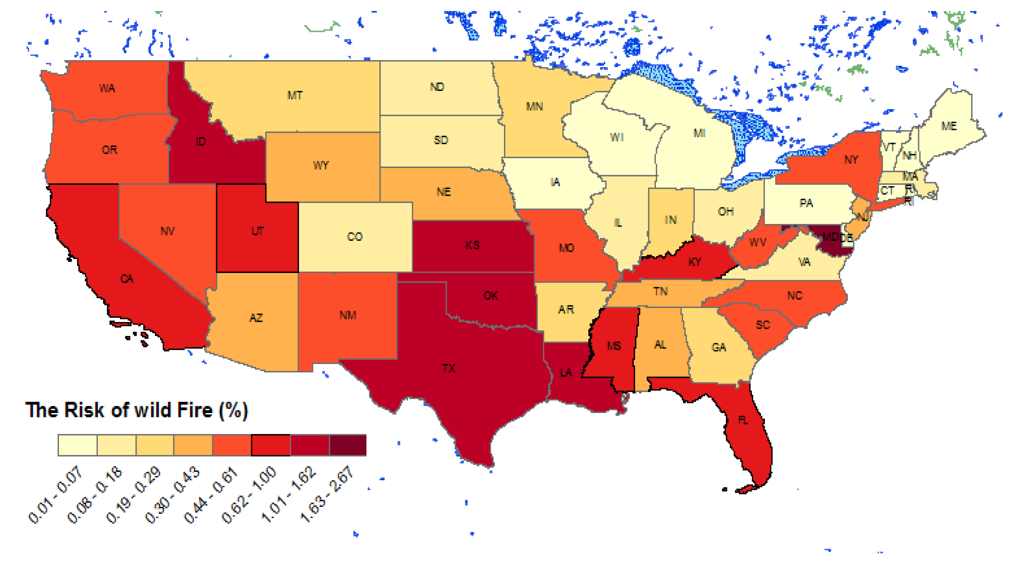
3.1. Factors Attributable to Wildfire Risk

Table 2 shows the average partial effects of various factors on wildfire risk based on the estimated fractional probit model. As suggested in Pan (2001) [30], we chose our model specification by comparing information criteria for GEE models, QIC and QICu, of which the smaller the better. For example, including quadratic terms for weather variables do not show improvements of the model performance (QICu = 55.256 for the full model including quadratic terms and 44.574 for the model without quadratic terms). Likewise, the AR(1) correlation structure outperforms other correlation matrix specifications according to the QIC statistics. In terms of the goodness of fit, our model shows that according to the Wald Chi square statistic, the null hypothesis that at least one coefficient is not zero is rejected at the 1% level, which implies that at least one covariate affects our model. For each covariate, p-values are calculated (Table 2).
Table 2. Marginal effect of various factors on wildfire risk in the continental US.
Independent VariableMarginal EffectStandard ERRp-Value
Pop (Population density, persons/km2)0.01100.00650.093
BIOM (Tree biomass density, Mg/ha)−0.01400.00450.004
HARV(Annual timber removal, m3/ha)0.00100.00170.466
MORT(Annual tree mortality, m3/ha)−0.00200.00410.640
SPT (Average spring monthly temperature, K)0.15000.06130.014
SMT (Average summer monthly temperature, K)0.45400.08000.000
FLT (Average fall monthly temperature, K)0.05400.08000.499
WNT (Average winter monthly temperature, K)0.12000.05000.015
SPP (monthly total spring precipitation, mm)−0.00030.00070.632
SMP (monthly total summer precipitation, mm)−0.00300.00090.005
FLP (monthly total fall precipitation mm)−0.00040.00060.519
WNP (monthly total winter precipitation, mm)−0.00030.00120.818
The regression result indicates that spring, summer, and winter temperatures, summer precipitation, and tree biomass density have a significant impact on wildfire risk at the 5% significance level, and that human population density is significant at the 10% level. Population density has a positive impact on wildfire risk. An increase in population density suggests increased human activity (interactions with the natural area) and thus heightened wildfire risk as most wildfires in the US are caused by humans. Surprisingly, an increase in tree biomass density shows a negative impact on wildfire risk. This might be partially because more and better wildfire prevention and protection measures are enforced in well stocked forests that have high commercial and ecosystem service values.
Rises in spring, summer, and winter temperatures intensify wildfire risk whereas an increase in summer precipitation reduces wildfire risk. Changes in these seasonal temperatures and precipitation not only alter vegetation (thus fuel type and structure) but also fuel moisture [31], thus affecting wildfire risk. The regression results also show that the magnitude of the temperature impact on wildfire risk is larger than that of the precipitation effect. Additionally, an increase in summer temperature has a much greater impact on wildfire risk than a rise in spring or winter temperature. Liu et al. [3] report that the highest fire potential in the U.S occurs in the summer when temperature is the highest. There are at least two reasons for this. First, wildfire is most active in the summer. Second, summer average temperature is higher than that of spring or winter. Thus, additional change in summer temperature would cause a more dramatic change in fuel moisture and thus a more detrimental impact on wildfire risk than a similar change in spring or winter temperature. Given the heterogeneity of impacts of seasonal temperatures and precipitation, changes in temperature and precipitation will have different impacts on wildfire risk at different locations.

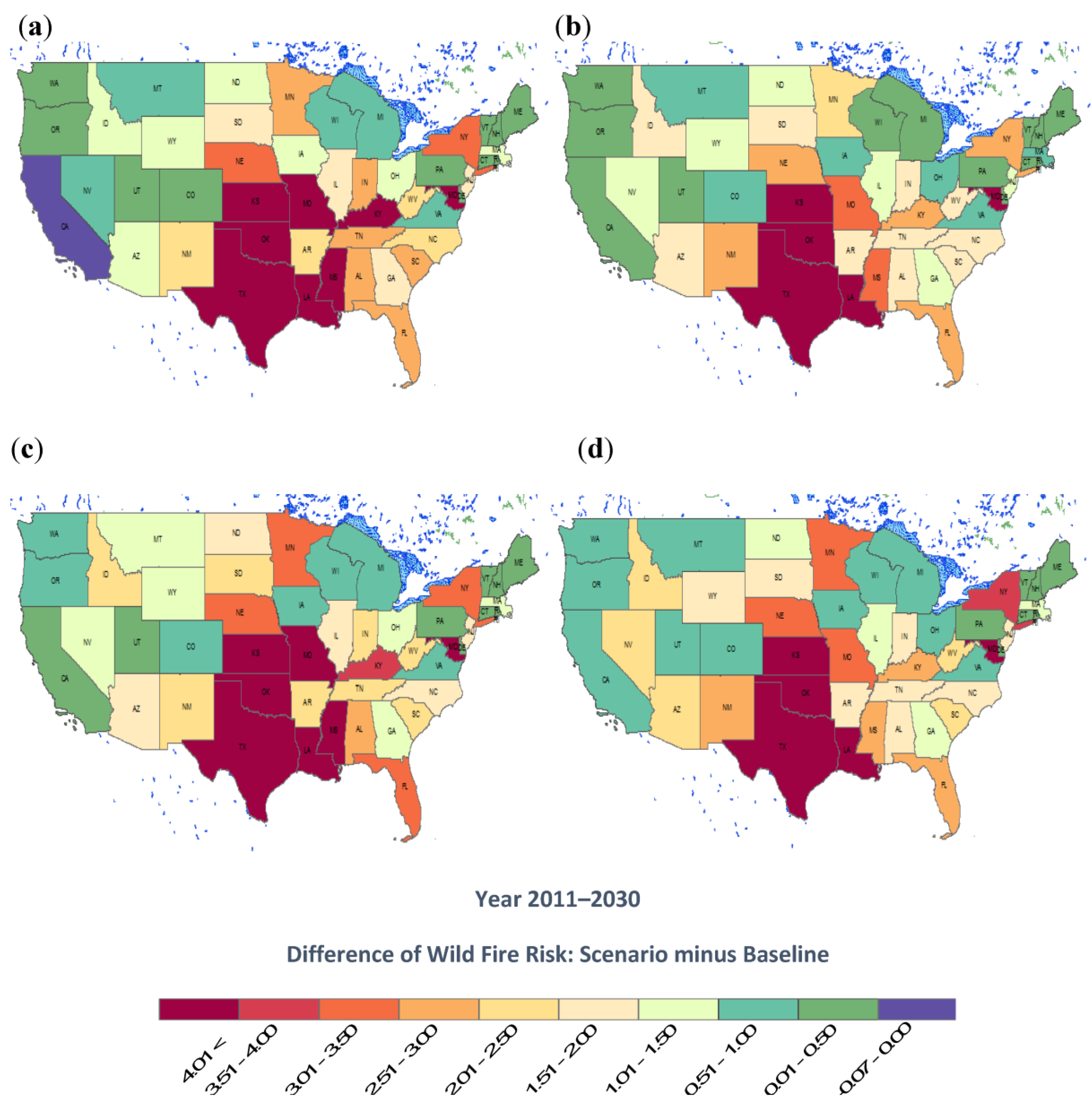
3.2. Climate Change Impact on Wildfire Risk

Figure 1 displays the annual average wildfire risk from 1991 to 1997 based on wildfire statistics [24]. We use this historical average as the baseline to compare the climate change impact. Figure 2 and Figure 3 show the changes in wildfire risk (relative to the baseline) under different climate change scenarios. These two figures are created by subtracting the historical wildfire risk (Figure 1) from the projected future wildfire risk under climate change for each state in the US. Figure 2 and Figure 3 show the projected change in average wildfire risk in the period from 2011 to 2030 and in the period from 2031 to 2050, respectively. According to our model projections, almost all states in the continental US would experience an increase in wildfire risk under both the moderate and rapid GHG accumulation scenarios. The highest risk would occur in the South Central states, including Texas, Oklahoma, Louisiana, and Kansas. The climate change impact would be more severe in the long run (2031–2050) than in the short run (2011–2030) because the magnitude of projected climate change is expected to be greater in the long run than in the short run due to the accumulation of GHG emissions. Additionally, the overall direction and spatial patterns of projected change in wildfire risk vary across the GCMs and the RCP scenarios. This implies considerable uncertainty associated the projections of climate change impact on wildfire risk [31].
Figure 1. Average annual wildfire risk from 1991 to 1997 in 48 continental US states. The wildfire risk is measured in the percent of area burned by wildfire in total forested area.
Forests 06 03197 g001
Some of our results echo those of previous studies which focus on specific regions in the US, particularly the Western US where the most severe impact of climate change on wildfire has been anticipated. The Harvard School of Engineering and Applied Science (SEAS) team estimate future wildfire activity in the Western US during 2046 to 2065 using GCMs based on the IPCC AR4 (fourth assessment report) scenarios [32]. They conclude that the biggest driver for fires in the future is temperature, so fires would increase in size if we meet large temperature increases overtime. Moreover, the fire season would start earlier (late April instead of mid-May) and end later (mid-October instead of early October) due to global climate change. However, our nationwide analysis suggests that the greatest impact of climate change on wildfire would occur in the South Central US rather than in the Western or Southwestern US.
Figure 2. (a) Change in wildfire risk relative to the baseline (historical average) with the future climate projected by the HadCM3 model under the RCP 4.5 scenario; (b) Change in wildfire risk relative to the baseline with the future climate projected by the NOAA-GFDL model under the RCP 4.5 scenario; (c) Change in wildfire risk relative to the baseline with the future climate projected by the HadCM3 model under the RCP 8.5 scenario; (d) Change in wildfire risk relative to the baseline with the future climate projected by the NOAA-GFDL model under the RCP 8.5 scenario. The changes in wildfire risk are calculated by subtracting the historical average wildfire risk from the projected future wildfire risk based on the climatic conditions projected by the GCMs. This figure indicates the short-run (2011–2030) impact of climate change on wildfire risk.
Forests 06 03197 g002
Figure 3. (a) Change in wildfire risk relative to the baseline (historical average) with the future climate projected by the HadCM3 model under the RCP 4.5 scenario; (b) Change in wildfire risk relative to the baseline with the future climate projected by the NOAA-GFDL model under the RCP 4.5 scenario; (c) Change in wildfire risk relative to the baseline with the future climate projected by the HadCM3 model under the RCP 8.5 scenario; (d) Change in wildfire risk relative to the baseline with the future climate projected by the NOAA-GFDL model under the RCP 8.5 scenario. The changes in wildfire risk are calculated by subtracting the historical average wildfire risk from the projected future wildfire risk based on the climatic conditions projected by the GCMs. This figure indicates the long-run (2031–2050) impact of climate change on wildfire risk.
Forests 06 03197 g003

4. Conclusions

We apply non-linear panel data modeling to establishing a statistical linkage between wildfire risk and climatic and other factors. The model is estimated by using the GEE method. This approach takes into account of the bounded nature of the dependent variable, wildfire risk that is fractional response variable. Additionally, the panel data model can better control for missing or unobserved variables and alleviate the multicollinearlity problem associated with correlated climate variables, while incorporating natural and human adaptations into the modeling. All these represent methodological innovations in modeling climate change impact on wildfire risk. Meanwhile, we simulate the impact of climate change on future wildfire risk using our regression model coupled with the future climates projected by two GCMs under two RCP scenarios.
According to our modeling results, both climate and non-climate variables are likely to affect wildfire risk. Wildfire risk would generally increase with an increase in temperature and a decrease in precipitation. Spring, summer, and winter temperatures in particular would have a significant impact on wildfire risk with summer temperature having the largest impact. This implies that climate change could greatly intensify wildfire risk particularly in the summer, the most active and severe wildfire season, and make the wildfire season longer, extending from spring to winter. On the other hand, precipitation increases would likely reduce wildfire risk. Temperature increases coupled with human population expansion could elevate wildfire risk as humans are a major source of wildfire ignitions.
Based on the future temperatures and precipitations predicted by the GCMs, future wildfire risk would increase in almost all states. The South Central states including Texas, Oklahoma, Louisiana, Kansas would experience the highest risk increase, and the climate change impact will be more severe in the long run (2031–2050) than in the short-run (2011–2030). This calls for more effective wildfire management strategies for all states in general and the South Central region in particular.
Our simulation results on the climate change impact on future wildfire risk demonstrate considerable variations across the future climate scenarios projected by the GCMs under the different RCP scenarios. The variations could stem from several sources. First, it is the uncertainty associated with the projections of future climate. The variations in the future climates projected by different GCMs are substantial even under the same RCP scenario, which contributes greatly to the variations in our projected impact of climate change on wildfire risk. Second, our regression model indicates that temperature in general has a positive impact on wildfire risk whereas precipitation tends to dampen wildfire risk. According to the simulation results from the GCMs, changes in temperature and precipitation (in both magnitude and direction) under climate change vary tremendously from location to location. This adds to the uncertainty in projecting climate change impact on wildfire risk, particularly given the difficulty in projecting future climate on a finer scale or at the local level. Third, our regression model is estimated using seven-year data due to the unavailability of consistently recorded nationwide wildfire data. Although the spatial variations in our data compensate for the limitation imposed by the short time series, using the data of a longer time series available in the future could improve the estimation of our regression model and thus the projections of climate change impact on wildfire risk. Hence, there is a need for future studies to address these uncertainties.
This study focuses on the impact of climatic conditions on wildfire risk. Although our data and modeling approach can incorporate some human response (e.g., adaptation) to wildfire into the analysis, national wildfire policy is not explicitly included in the model. National wildfire policy can interact with wildfire risk; future studies can also explore their interaction. Additionally, to overcome the limitations of current GCMs, future studies can apply statistical downscaling models, such as Multivariate Adapted Constructed Analogs (MACA) [33].

Acknowledgments

This study is financially supported in part by the USDA National Institute of Food and Agriculture (Award #2011-68002-30185), and Texas A & M AgriLife Research.

Author Contributions

Jianbang Gan designed the study and the research method, and provided essential comments to improve the modeling and the manuscript. Hyunjin An implemented statistical modeling and climate change impact simulations, and wrote the first draft of the manuscript. Sung Ju Cho processed the climate data and helped with statistical modeling. All authors contributed to the writing of the manuscript.

Conflicts of Interest

The authors declare no conflict of interest.

References

  1. IPCC Working Group. Climate Change 2013: The Physical Science Basis; Contribution of Working Group I to the Fifth Assessment Report of the Intergovernmental; Cambridge University Press: New York, NY, USA, 2013. [Google Scholar]
  2. Westerling, A.L.; Hidalgo, H.G.; Cayan, D.R.; Swetnam, T.W. Warming and earlier spring increase western U.S. forest wildfire activity. Science 2006, 313, 940–943. [Google Scholar] [CrossRef] [PubMed]
  3. Liu, Y.; Stanturf, J.; Goodrick, S. Trends in global wildfire potential in a changing climate. For. Ecol. Manag. 2010, 259, 685–697. [Google Scholar] [CrossRef]
  4. Jeremy, S.; Littell, D.M. Climate and wildfire area burned in western U.S. ecoprovinces, 1916–2003. Ecol. Appl. Publ. Ecol. Soc. Am. 2009, 19, 1003–1021. [Google Scholar]
  5. Moritz, M.A.; Parisien, M.-A.; Batllori, E.; Krawchuk, M.A.; van Dorn, J.; Ganz, D.J.; Hayhoe, K. Climate change and disruptions to global fire activity. Ecosphere 2012, 3. art49. [Google Scholar] [CrossRef]
  6. Dennison, P.E.; Brewer, S.C.; Arnold, J.D.; Moritz, M.A. Large wildfire trends in the western United States, 1984–2011. Geophys. Res. Lett. 2014, 41. [Google Scholar] [CrossRef]
  7. Preisler, H.; Westerling, A.L.; Gebert, K.M.; Munoz-Arriola, F.; Holmes, T.P. Spatially explicit forecasts of large wildland fire probability and suppression costs for California. Int. J. Wildland Fire 2011, 20, 508–517. [Google Scholar] [CrossRef]
  8. Hardin, J.W. Generalized Estimating Equations (GEE). In Encyclopedia of Statistics in Behavioral Science; John Wiley & Sons, Ltd.: Hoboken, NJ, USA, 2005. [Google Scholar]
  9. Zeileis, A. Econometric Computing with HC and HAC Covariance Matrix Estimators. Available online: http://epub.wu.ac.at/520/ (accessed on 18 June 2015).
  10. Baltagi, B.H. Econometric Analysis of Panel Data, 4th ed.; Wiley: Chichester, UK; Hoboken, NJ, USA, 2008. [Google Scholar]
  11. Hsiao, C. Analysis of Panel Data; Cambridge University Press: New York, NY, USA, 2014. [Google Scholar]
  12. Gan, J. New Research on Forest Ecosystems; Nova Publishers: Hauppauge, NY, USA, 2005. [Google Scholar]
  13. Papke, L.E.; Wooldridge, J.M. Econometric methods for fractional response variables with an application to 401(k) plan participation rates. J. Appl. Econ. 1996, 11, 619–632. [Google Scholar] [CrossRef]
  14. Westerling, A.L.; Bryant, B.P. Climate change and wildfire in California. Clim. Chang. 2008, 87, S231–S249. [Google Scholar] [CrossRef]
  15. Hardin, J.W.; Hilbe, J.M. Generalized Estimating Equations, 2nd ed.; Chapman and Hall/CRC: Boca Raton, FL, USA, 2012. [Google Scholar]
  16. Cushman, S.A.; Chase, M.; Griffin, C. Elephants in Space and Time. Oikos 2005, 109, 331–341. [Google Scholar] [CrossRef]
  17. Brillinger, D.R.; Preisler, H.K.; Benoit, J.W. Probabilistic risk assessment for wildfires. Environmetrics 2006, 17, 623–633. [Google Scholar] [CrossRef]
  18. Gibbons, R.D.; Hedeker, D.; DuToit, S. Advances in analysis of longitudinal data. Annu. Rev. Clin. Psychol. 2010, 6, 79–107. [Google Scholar] [CrossRef] [PubMed]
  19. IPCC Data Distribution Center. Available online: http://www.ipcc-data.org/guidelines/pages/gcm_guide.html (accessed on 25 August 2014).
  20. Dietrich-Egensteiner, W. A Beginner’s Guide to the IPCC Climate Change Reports. Available online: http://www.popularmechanics.com/science/environment/climate-change/a-beginners-guide-to-the-ipcc-climate-change-reports-15991849 (accessed on 23 July 2015).
  21. Fitzmaurice, G.M.; Laird, N.M.; Ware, J.H. Applied Longitudinal Analysis, 2nd ed.; Wiley: Hoboken, NJ, USA, 2005. [Google Scholar]
  22. Anderson, H.E. Aids to Determining Fuel Models for Estimating Fire Behavior; U.S. Department of Agriculture, Forest Service, Intermountain Forest and Range Experiment Station: Ogden, UT, USA, 1981. [Google Scholar]
  23. Rothermel, R.C.; Philpot, C.W. Predicting changes in chaparral flammability. Available online: http://texasamcolstattx.library.ingentaconnect.com/content/saf/jof/1973/00000071/00000010/art00013 (accessed on 23 July 2015).
  24. United States Department of Agriculture, Forest Service. 1991–1997 Wildland Fire Statistics; USDA Forest Service, Fire and Aviation Management: Washington, DC, USA, 1998. [Google Scholar]
  25. Westerling, A.L.; Swetnam, T.W. Interannual to decadal drought and wildfire in the western United States. Eos Trans. Am. Geophys. Union 2003, 84, 545–555. [Google Scholar] [CrossRef]
  26. Whitlock, C.; Shafer, S.L.; Marlon, J. The role of climate and vegetation change in shaping past and future fire regimes in the northwestern US and the implications for ecosystem management. For. Ecol. Manag. 2003, 178, 5–21. [Google Scholar] [CrossRef]
  27. Climate at a Glance. Available online: http://www.ncdc.noaa.gov/cag/ (accessed on 1 February 2015).
  28. Smith, W.B. Forest Resources of the United States, 1997. [Microform]; General Technical Report NC: 219; North Central Research Station, Forest Service—U.S. Depatment of Agriculture: St. Paul, MN, USA, 2001. [Google Scholar]
  29. Brekke, L.; Thrasher, B.L.; Maurer, E.P.; Pruitt, T. Downscaled CMIP3 and CMIP5 Climate Projections: Release of Downscaled CMIP5 Climate Projections, Comparison with Preceding Information, and Summary of User Needs; U.S. Department of the Interior, Bureau of Reclamation, Technical Service Center: Denver, CO, USA. Available online: http://gdodcp.ucllnl.org/downscaled_cmip_projections (accessed on 13 July 2014).
  30. Pan, W. Akaike’s Information criterion in generalized estimating equations. Biometrics 2001, 57, 120–125. [Google Scholar] [CrossRef] [PubMed]
  31. Schneider, S.H. Climate Change Science and Policy; Island Press: Washington, DC, USA, 2009. [Google Scholar]
  32. Yue, X.; Mickley, L.J.; Logan, J.A.; Kaplan, J.O. Ensemble projections of wildfire activity and carbonaceous aerosol concentrations over the western United States in the mid-21st century. Atmos. Environ. 2013, 77, 767–780. [Google Scholar] [CrossRef] [PubMed]
  33. Abatzoglou, J.T.; Brown, T.J. A comparison of statistical downscaling methods suited for wildfire applications. Int. J. Climatol. 2012, 32, 772–780. [Google Scholar] [CrossRef]

