
Modeling of Two Different Water Uptake Approaches for Mono- and Mixed-Species Forest Stands

Abstract
:1. Introduction
2. Material and Methods
2.1. Forest Growth Model 4C
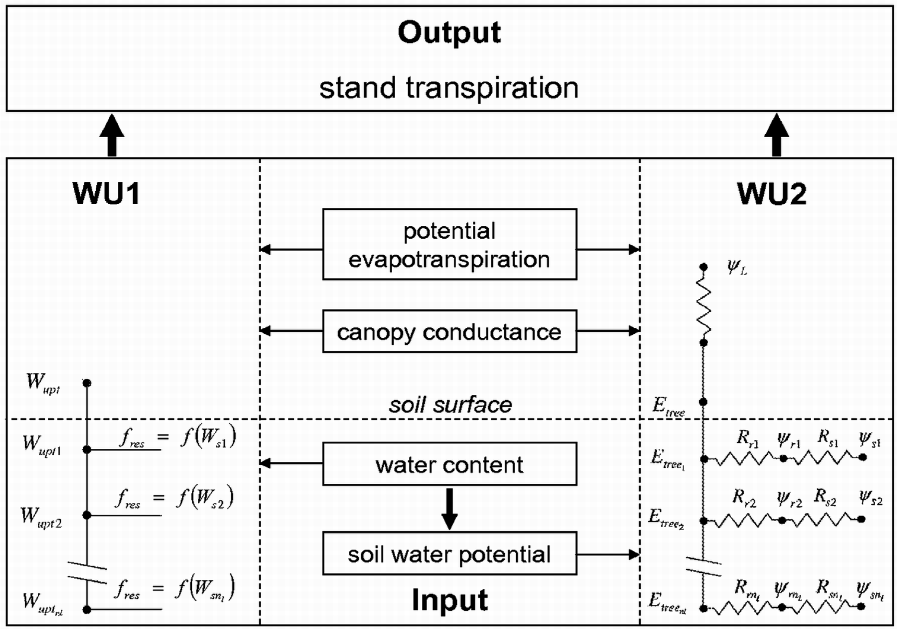
2.2. Modeling Water Uptake
2.2.1. Empirical Water Uptake Approach—WU1

2.2.2. Process-Based Water Uptake Approach—WU2
2.3. Forest Stands and Site Conditions

| 1951 | 1994 | ||||||||
|---|---|---|---|---|---|---|---|---|---|
| Age (years) | dg (cm) | hg (m) | Stock (m3) | Age (years) | dg (cm) | hg (m) | Stock (m3) | ||
| P1 | pine | 18 | 9.0 | 13.7 | 209 | 62 | 29.8 | 25.9 | 458 |
| P2 | pine | 29 | 10.5 | 14.0 | 205 | 73 | 28.3 | 24.3 | 347 |
| M1 | pine | 85 | 31.8 | 25.0 | 258 | ||||
| oak | 85 | 20.9 | 20.0 | 136 | |||||
| M2 | pine | 65 | 24.8 | 23.1 | 159 | ||||
| oak | 70 | 21.2 | 22.4 | 239 | |||||
| Site | Soil Type | Soil Depth (cm) | WsFC (mm) | WsAW (mm) | C/N | ps (%) | pc (%) |
|---|---|---|---|---|---|---|---|
| P1 | brunic arenosol | 270 | 217 | 119 | 22 | 90–100 | 0–5 |
| P2 | brunic arenosol | 255 | 237 | 93 | 21 | 50–100 | 0–17 |
| M1 | brunic arenosol | 308 | 526 | 369 | 21 | 91–98 | 1–4 |
| M2 | brunic arenosol | 305 | 607 | 395 | 15 | 75–97 | 2–9 |
2.4. Climate Data
| Site | Ty (°C) | Tg (°C) | Py (mm) | Pg (mm) |
|---|---|---|---|---|
| P1 | 8.1 | 13.8 | 600 | 344 |
| P2 | 8.5 | 14.7 | 550 | 309 |
| M1 | 8.5 | 15.2 | 531 | 255 |
| M2 | 8.9 | 16.2 | 521 | 267 |
2.5. Measured Data
2.5.1. Xylem Sap Flow Data
| Site | Data | Period | Source |
|---|---|---|---|
| P1 |
| 06/1998–10/1999 | [40] |
| 1997–2004 | [41,42,43] | ||
| until 2004 | [44] | ||
| P2 |
| 1997–2004 | [41,42,43] |
| until 2004 | [44] | ||
| M1 |
| until 2006 | [45] |
| M2 |
| until 2006 | [45] |
2.5.2. Soil Water Content
2.5.3. Tree Ring Data
2.6. Validation Procedure
2.7. Statistical Analysis
- criteria I
- r* = r × 100 (if r < 0; r* = 0)
- criteria II
- Gxy* = Gxy
- criteria III
- SI* = 100 − (|SIsim − SImeas|)/SImeas × 100)
- criteria IV
- DI* = DI
3. Results
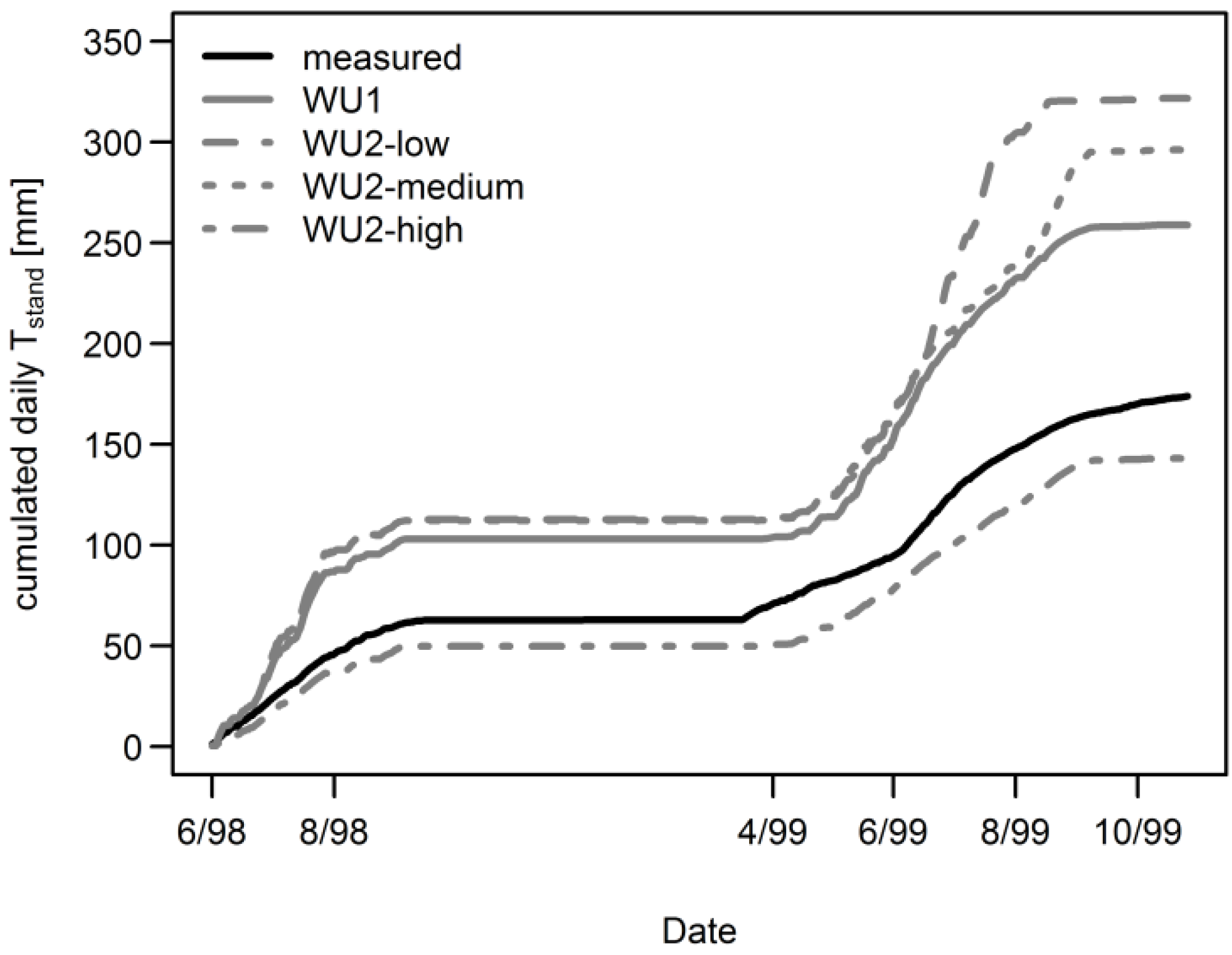
3.1. Daily Xylem Sap Flow


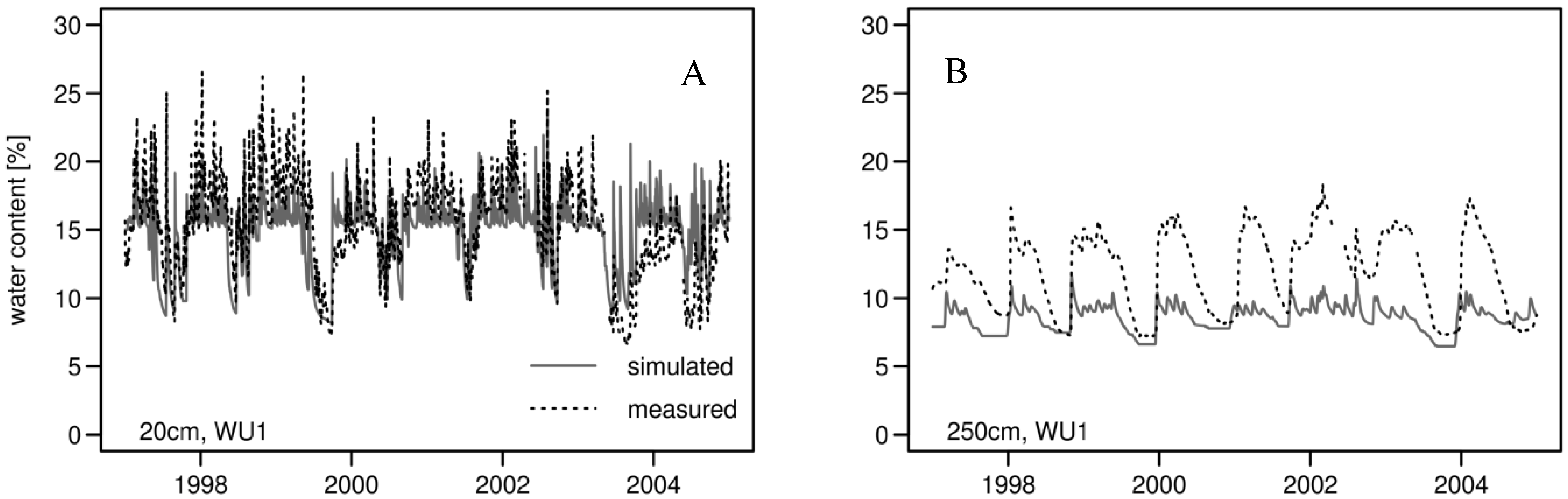
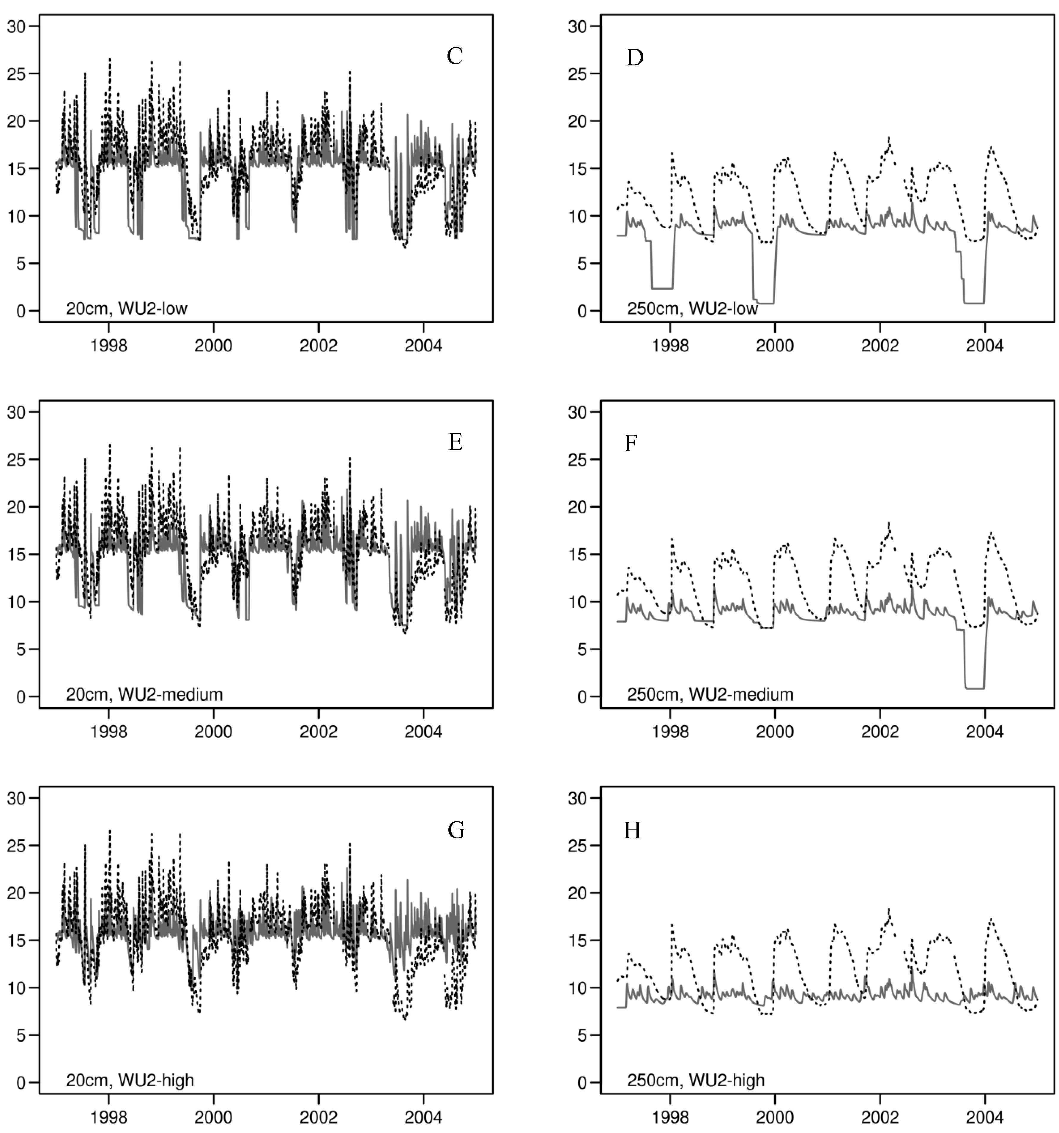
3.2. Daily Soil Water Content
| Soil Depth | R2 | Mean Soil Water Content [%] | CV of Soil Water Content | |||
|---|---|---|---|---|---|---|
| [cm] | Simulated | Measured | Simulated | Measured | ||
| WU1 | 20 | 0.50 | 14.75 | 15.32 | 0.17 | 0.23 |
| 70 | 0.41 | 9.95 | 10.90 | 0.12 | 0.11 | |
| 250 | 0.55 | 8.55 | 11.88 | 0.12 | 0.25 | |
| WU2-low | 20 | 0.51 | 14.37 | 15.32 | 0.23 | 0.23 |
| 70 | 0.35 | 9.82 | 10.90 | 0.14 | 0.11 | |
| 250 | 0.36 | 7.56 | 11.88 | 0.38 | 0.25 | |
| WU2-medium | 20 | 0.52 | 14.57 | 15.32 | 0.20 | 0.23 |
| 70 | 0.38 | 9.97 | 10.90 | 0.12 | 0.11 | |
| 250 | 0.31 | 8.36 | 11.88 | 0.23 | 0.25 | |
| WU2-high | 20 | 0.32 | 15.65 | 15.32 | 0.10 | 0.23 |
| 70 | 0.43 | 10.43 | 10.90 | 0.08 | 0.11 | |
| 250 | 0.07 | 9.15 | 11.88 | 0.07 | 0.25 | |


3.3. Annual Tree Ring Data
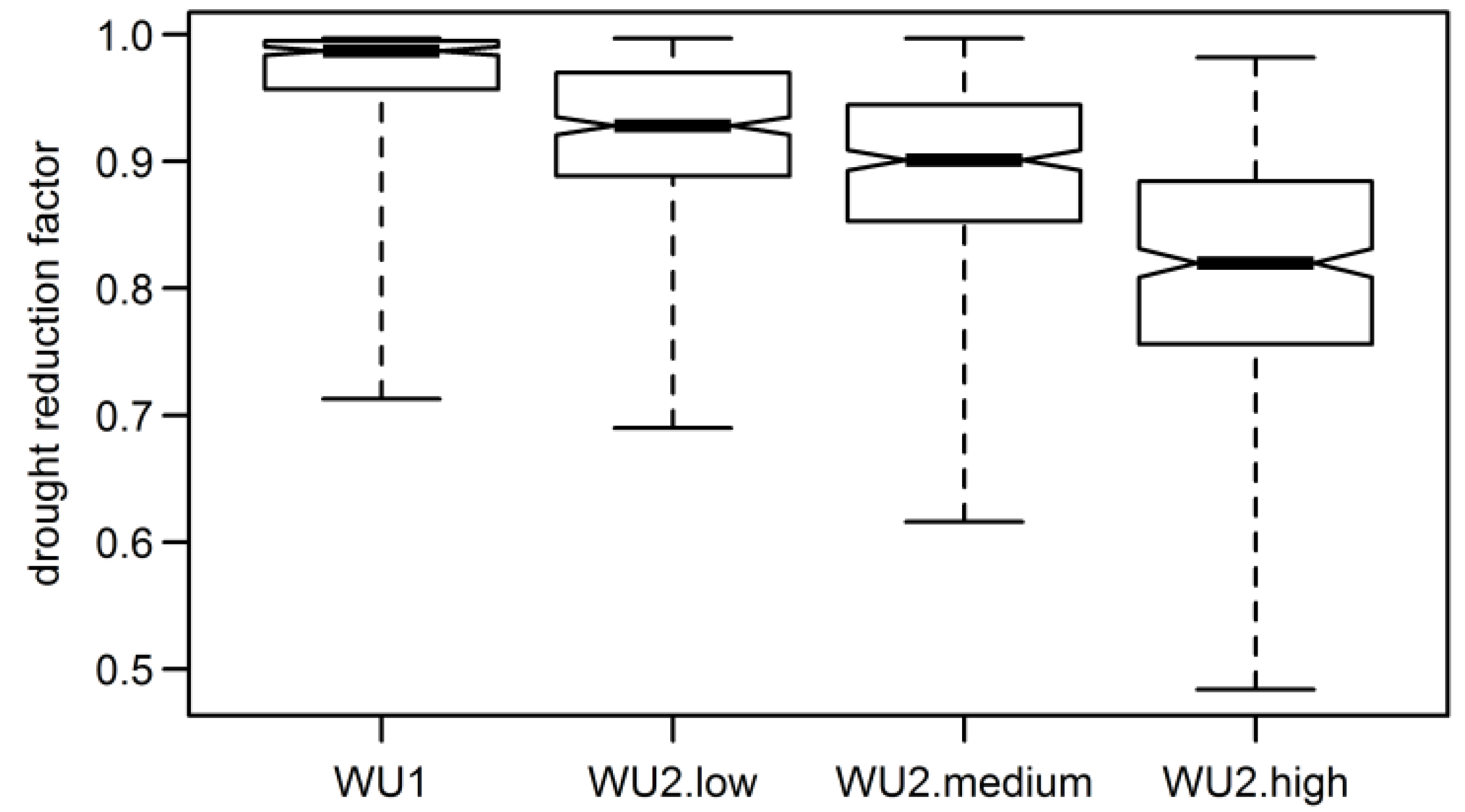
3.4. Aggregated Datasets
| Model | Mean Compliance | WU2-Low | WU2-Medium | WU2-High |
|---|---|---|---|---|
| 47.3 | 54.6 | 56.7 | ||
| WU1 | 41.9 | 0.81 | 0.16 | 0.08 |
| WU2-low | 47.3 | 0.62 | 0.42 | |
| WU2-medium | 54.6 | 0.99 |
4. Discussion
4.1. Water Uptake and Root Resistance
4.2. Short-Term Performance of Root Water Uptake Approaches
4.3. Effect of Root Water Uptake Approach on Diameter Growth
5. Conclusions
Acknowledgments
Author Contributions
Conflicts of Interest
References
- Alcamo, J.; Moreno, J.M.; Nováky, B.; Bindi, M.; Corobov, R.; Devoy, R.J.N.; Giannakopoulos, C.; Martin, E.; Olesen, J.E.; Shvidenko, A.; et al. Europe. In Climate Change 2007: Impacts, Adaptation and Vulnerability; Contribution of Working Group II to the Fourth Assessment Report of the Intergovernmental Panel on Climate Change; Parry, M.L., Palutikof, J.P., van der Linden, P.J., Hanson, C.E., Eds.; Cambridge University Press: Cambridge, UK, 2007; pp. 541–580. [Google Scholar]
- Lasch, P.; Badeck, F.W.; Suckow, F.; Lindner, M.; Mohr, P. Model-Based analysis of management alternatives at stand and regional level in Brandenburg (Germany). For. Ecol. Manag. 2005, 207, 59–74. [Google Scholar] [CrossRef]
- Lindner, M.; Cramer, W. German forest sector under global change: An interdisciplinary impact assessment. Forstwiss. Cent. 2002, 121, 3–17. [Google Scholar]
- Pussinen, A.; Nabuurs, G.J.; Wieggers, H.J.J.; Reinds, G.J.; Wamelink, G.W.W.; Kros, J.; Mol-Dijkstra, J.P.; de Vries, W. Modelling long-term impacts of environmental change on mid- and high-latitude European forests and options for adaptive forest management. For. Ecol. Manag. 2009, 258, 1806–1813. [Google Scholar] [CrossRef]
- Reyer, C.; Lasch-Born, P.; Suckow, F.; Gutsch, M.; Murawski, A.; Pilz, T. Projections of regional changes in forest net primary productivity for different tree species in Europe driven by climate change and carbon dioxide. Ann. For. Sci. 2014, 71, 211–225. [Google Scholar]
- Farquhar, G.D.; Sharkey, T.D. Stomatal conductance and phostosynthesis. Annu. Rev. Plant Physiol. 1982, 33, 317–345. [Google Scholar] [CrossRef]
- Jarvis, A.J.; Davies, W.J. The coupled response of stomatal conductance to photosynthesis and transpiration. J. Exp. Bot. 1998, 49, 399–406. [Google Scholar] [CrossRef]
- Lindner, M.; Fitzgerald, J.B.; Zimmermann, N.E.; Reyer, C.; Delzon, S.; van der Maaten, E.; Schelhaas, M.J.; Lasch-Born, P.; Eggers, J.; van der Maaten-Theunissen, M.; et al. Climate Change and European Forests: What do we know, what are the uncertainties, and what are the implications for forest management? J. Environ. Manag. 2014, 146, 69–83. [Google Scholar] [CrossRef] [PubMed]
- Scarascia-Mugnozza, G.; Oswald, H.; Piussi, P.; Radoglou, K. Forests of the Mediterranean region: Gaps in knowledge and research needs. For. Ecol. Manag. 2000, 132, 97–109. [Google Scholar] [CrossRef]
- Breda, N.; Huc, R.; Granier, A.; Dreyer, E. Temperate forest trees and stands under severe drought: A review of ecophysiological responses, adaptation processes and long-term consequences. Ann. For. Sci. 2006, 63, 625–644. [Google Scholar] [CrossRef]
- Galiano, L.; Martínez-Vilalta, J.; Lloret, F. Drought-Induced Multifactor Decline of Scots Pine in the Pyrenees and Potential Vegetation Change by the Expansion of Co-occurring Oak Species. Ecosystems 2010, 13, 978–991. [Google Scholar] [CrossRef]
- Poyatos, R.; Martinez-Vilalta, J.; Cermak, J.; Ceulemans, R.; Granier, A.; Irvine, J.; Kostner, B.; Lagergren, F.; Meiresonne, L.; Nadezhdina, N.; et al. Plasticity in hydraulic architecture of Scots pine across Eurasia. Oecologia 2007, 153, 245–259. [Google Scholar]
- Rebetez, M.; Dobbertin, M. Climate change may already threaten Scots pine stands in the Swiss Alps. Theor. Appl. Climatol. 2004, 79, 1–9. [Google Scholar] [CrossRef]
- Cruiziat, P.; Cochard, H.; Ameglio, T. Hydraulic architecture of trees: Main concepts and results. Ann. For. Sci. 2002, 59, 723–752. [Google Scholar] [CrossRef]
- Holst, J.; Grote, R.; Offermann, C.; Ferrio, J.P.; Gessler, A.; Mayer, H.; Rennenberg, H. Water fluxes within beech stands in complex terrain. Int. J. Biometeorol. 2010, 54, 23–36. [Google Scholar] [CrossRef] [PubMed]
- Keenan, T.; Sabate, S.; Gracia, C. Soil water stress and coupled photosynthesis–conductance models: Bridging the gap between conflicting reports on the relative roles of stomatal, mesophyll conductance and biochemical limitations to photosynthesis. Agric. For. Meteorol. 2010, 150, 443–453. [Google Scholar] [CrossRef]
- Keenan, T.; Garcia, R.; Friend, A.D.; Zaehle, S.; Gracia, C.; Sabate, S. Improved understanding of drought controls on seasonal variation in Mediterranean forest canopy CO2 and water fluxes through combined in situ measurements and ecosystem modelling. Biogeosciences 2009, 6, 1423–1444. [Google Scholar] [CrossRef]
- Wang, Y.; Bauerle, W.L.; Reynolds, R.F. Predicting the growth of deciduous tree species in response to water stress: FVS-BGC model parameterization, application, and evaluation. Ecol. Model. 2008, 217, 139–147. [Google Scholar] [CrossRef]
- Reyer, C.; Leuzinger, S.; Rammig, A.; Wolf, A.; Bartholomeus, R.P.; Bonfante, A.; de Lorenzi, F.; Dury, M.; Gloning, P.; Abou Jaoudé, R.; et al. A plant’s perspective of extremes: Terrestrial plant responses to changing climatic variability. Glob. Chang. Biol. 2013, 19, 75–89. [Google Scholar] [CrossRef] [PubMed]
- Williams, M.; Rastetter, E.B.; Fernandes, D.N.; Goulden, M.L.; Wofsy, S.C.; Shaver, G.R.; Melillo, J.M.; Munger, J.W.; Fan, S.M.; Nadelhoffer, K.J.; et al. Modelling the soil-plant-atmosphere continuum in a Quercus-Acer stand at Harvard forest: The regulation of stomatal conductance by light, nitrogen and soil/plant hydraulic properties. Plant Cell Environ. 1996, 19, 911–927. [Google Scholar] [CrossRef]
- Campbell, G.S. Simulations of Water Uptake by Plant Roots. In Modeling Plant and Soil Systems; Hanks, J., Ritchie, J.T., Eds.; American Society of Agronomy: Madison, WI, USA, 1991; pp. 273–285. [Google Scholar]
- Doussan, C.; Vercambre, G.; Pages, L. Modelling of the hydraulic architecture of root systems: An integrated approach to water absorption—Distribution of axial and radial conductances in maize. Ann. Bot. 1998, 81, 225–232. [Google Scholar]
- Grant, R.F.; Arain, A.; Arora, V.; Barr, A.; Black, T.A.; Chen, J.; Wang, S.; Yuan, F.; Zhang, Y. Intercomparison of techniques to model high temperature effects on CO2 and energy exchange in temperate and boreal coniferous forests. Ecol. Model. 2005, 188, 217–252. [Google Scholar] [CrossRef]
- Hacke, U.G.; Sperry, J.S.; Ewers, B.E.; Ellsworth, D.S.; Schäfer, K.V.R.; Oren, R. Influence of soil porosity on water use in Pinus taeda. Oecologia 2000, 124, 495–505. [Google Scholar] [CrossRef]
- Williams, M.; Bond, B.J.; Ryan, M.G. Evaluating different soil and plant hydraulic constraints on tree function using a model and sap flow data from ponderosa pine. Plant Cell Environ. 2001, 24, 679–690. [Google Scholar] [CrossRef]
- Williams, M.; Law, B.E.; Anthoni, P.M.; Unsworth, M.H. Use of a simulation model and ecosystem flux data to examine carbon-water interactions in ponderosa pine. Tree Physiol. 2001, 21, 287–298. [Google Scholar]
- Grote, R.; Suckow, F. Integrating dynamic morphological properties into forest growth modeling. I. Effects on water balance and gas exchange. For. Ecol. Manag. 1998, 112, 101–119. [Google Scholar] [CrossRef]
- Kirschbaum, M.U.F. CenW, a forest growth model with linked carbon, energy, nutrient and water cycles. Ecol. Model. 1999, 118, 17–59. [Google Scholar] [CrossRef]
- Beniston, M. Weather and Climate Extremes: Where Can Dendrochronology Help? In Tree Rings and Natural Hazards: A State-of-Art; Stoffel, M., Bollschweiler, M., Butler, D.R., Luckman, B.H., Eds.; Springer: Dordrecht, The Netherlands; Heidelberg, Germany, 2010; pp. 401–413. [Google Scholar]
- Bugmann, H.; Grote, R.; Lasch, P.; Lindner, M.; Suckow, F. A new forest gap model to study the effects of environmental change on forest structure and functioning. Impacts of Global Change on Tree Physiology and Forest Ecosystems. In Proceedings of the International Conference on Impacts of Global Change on Tree Physiology and Forest Ecosystems, Wageningen, The Netherlands, 26–29 November 1996; Mohren, G.M.J., Kramer, K., Sabate, S., Eds.; Kluwer Academic Publisher: Dordrecht, The Netherlands, 1997; pp. 255–261. [Google Scholar]
- Lasch, P.; Lindner, M.; Erhard, M.; Suckow, F.; Wenzel, A. Regional impact assessment on forest structure and functions under climate change—The Brandenburg case study. For. Ecol. Manag. 2002, 162, 73–86. [Google Scholar]
- Haxeltine, A.; Prentice, I.C. BIOME3: An equilibrium terrestrial biosphere model based on ecophysiological constraints, resource availability and competition among plant functional types. Glob. Biogeochem. Cycles 1996, 10, 693–709. [Google Scholar] [CrossRef]
- Schaber, J.; Badeck, F.W. Physiology based phenology models for forest tree species in Germany. Int. J. Biometeorol. 2003, 47, 193–201. [Google Scholar]
- Glugla, G. Berechnungsverfahren zur Ermittlung des aktuellen Wassergehaltes und Gravitationswasserabflusses im Boden. Albrecht-Thaer-Archiv 1969, 13, 371–376. [Google Scholar]
- Koitzsch, R. Schätzung der Bodenfeuchte aus meteorologischen Daten, Boden- und Pflanzenparametern mit einem Mehrschichtmodell. Z. Meteorol. 1977, 27, 302–306. [Google Scholar]
- DVWK. Ermittlung der VERDUNSTUNG von Land- und Wasserflächen; Wirtschafts- und Verlagsgesellschaft Gas und Wasser mbH: Bonn, Germany, 1996; p. 134. [Google Scholar]
- Chen, C.W. The response of plants to interacting stresses: PGSM Version 1.3 Model Documentation (TR-101880); Report, OSTI ID: 6889091; Electric Power Research Institute: Palo Alto, CA, USA, 1993; p. 127. [Google Scholar]
- VanGenuchten, M.T. A closed-form equation for predicting the hydraulic conductivity of unsaturated soils. Soil Sci. Soc. Am. J. 1980, 44, 892–898. [Google Scholar]
- Granier, A. Une nouvelle méthode pour la mesure du flux de sève brute dans le tronc des arbres. Ann. Sci. For. 1985, 42, 193–200. [Google Scholar] [CrossRef]
- Lüttschwager, D.; Rust, S.; Wulf, M.; Forker, J.; Hüttl, R.F. Tree canopy and herb layer transpiration in three Scots pine stands with different stand structures. Ann. For. Sci. 1999, 56, 265–274. [Google Scholar]
- Landeskompetenzzentrum Forst Eberswalde, Forstliche-Umweltkontrolle. Available online: www.forstliche-umweltkontrolle-bb.de/index.php (accessed on 19 May 2015).
- Badeck, F.W.; Beese, F.; Berthold, D.; Einert, P.; Jochheim, H.; Kallweit, R.; Konopatzky, A.; Lasch, P.; Meesenburg, H.; Meiwes, K.-J.; et al. Parametrisierung, Kalibrierung und Validierung von Modellen des Kohlenstoffumsatzes in Waldökosystemen und deren Böden. DE 2003/2004 BB 5, DE 2003/2004 BY 4, DE 2003/2004 NI 6; F.F. C2-Projekte, Bayerische Landesanstalt für Wald und Forstwirtschaft (LWF), Institut für Bodenkunde und Waldernährung der Universität Göttingen (IBW), Landesforstanstalt Eberswalde (LFE), Leibniz-Zentrum für Agrarlandschaftsforschung (ZALF), Nordwestdeutsche Forstliche Versuchsanstalt (NW-FVA), Potsdam-Institut für Klimafolgenforschung (PIK): Potsdam, Germany, 2007; p. 110. [Google Scholar]
- Meiwes, K.-J.; Badeck, F.W.; Beese, F.; Berthold, D.; Einert, P.; Jochheim, H.; Kallweit, R.; Konopatzky, A.; Lasch, P.; Meesenburg, H.; et al. Kohlenstoffumsatz in Waldökosystemen und deren Böden. Parametrisierung, Kalibrierung und Validierung von Modellen. AFZ/Der Wald 2007, 20, 1076–1078. [Google Scholar]
- Beck, W. Growth patterns of forest stands—The response towards pollutants and climatic impact. iForest 2009, 2, 4–6. [Google Scholar] [CrossRef]
- Schröder, J.; Löffler, S.; Michel, A.; Kätzel, R. Genetische Differenzierung, Zuwachsentwicklung und Witterungseinfluß in Mischbeständen von Traubeneiche und Kiefer. Forst Holz 2009, 64, 18–24. [Google Scholar]
- Maechler, M.; Rousseeuw, P.; Struyf, A.; Hubert, M.; Hornik, K. Cluster Analysis Basics and Extensions. R Package, Version 2.0.1; Available online: http://cran.r-project.org/web/packages/cluster/citation.html (accessed on 21 March 2015).
- R Development Core Team. R: A Language and Environment for Statistical Computing; R Foundation for Statistical Computing: Vienna, Austria, 2009; ISBN 3-900051-07-0; Available online: http://www.R-project.org (accessed on 3 June 2015).
- McGill, R.; Tukey, J.W.; Larsen, W.A. Variations of box plots. Am. Stat. 1978, 32, 12–16. [Google Scholar]
- Coners, H. Wasseraufnahme und artspezifische hydraulische Eigenschaften der Feinwurzeln von Buche, Eiche und Fichte: In situ-Messungen an Altbäumen. Ph.D. Thesis, Mathematisch-Naturwissenschaftliche Fakultäten der Georg-August-Universität zu Göttingen, Göttingen, Germany, 2001. [Google Scholar]
- Kostner, B.; Biron, P.; Siegwolf, R.; Granier, A. Estimates of water vapor flux and canopy conductance of Scots pine at the tree level utilizing different xylem sap flow methods. Theor. Appl. Climatol. 1996, 53, 105–113. [Google Scholar] [CrossRef]
- Wilson, K.B.; Hanson, P.J.; Mulholland, P.J.; Baldocchi, D.D.; Wullschleger, S.D. A comparison of methods for determining forest evapotranspiration and its components: Sap-Flow, soil water budget, eddy covariance and catchment water balance. Agric. For. Meteorol. 2001, 106, 153–168. [Google Scholar]
- Bittner, S.; Talkner, U.; Kramer, I.; Beese, F.; Holscher, D.; Priesack, E. Modeling stand water budgets of mixed temperate broad-leaved forest stands by considering variations in species specific drought response. Agric. For. Meteorol. 2010, 150, 1347–1357. [Google Scholar] [CrossRef]
- Granier, A.; Loustau, D. Measuring and Modeling the transpiration of a maritime pine canopy from sap-flow data. Agric. For. Meteorol. 1994, 71, 61–81. [Google Scholar]
- Lundblad, M.; Lindroth, A. Stand transpiration and sapflow density in relation to weather, soil moisture and stand characteristics. Basic Appl. Ecol. 2002, 3, 229–243. [Google Scholar]
- Hanson, P.J.; Amthor, J.S.; Wullschleger, S.D.; Wilson, K.B.; Grant, R.F.; Hartley, A.; Hu, D.; Hunt, J.E.R.; Johnson, D.W.; Kimball, J.S.; et al. Oak forest carbon and water simulations: Model intercomparisons and evaluations against independent data. Ecol. Monogr. 2004, 74, 443–489. [Google Scholar] [CrossRef]
© 2015 by the authors; licensee MDPI, Basel, Switzerland. This article is an open access article distributed under the terms and conditions of the Creative Commons Attribution license (http://creativecommons.org/licenses/by/4.0/).
Share and Cite
Gutsch, M.; Lasch-Born, P.; Suckow, F.; Reyer, C.P.O. Modeling of Two Different Water Uptake Approaches for Mono- and Mixed-Species Forest Stands. Forests 2015, 6, 2125-2147. https://doi.org/10.3390/f6062125
Gutsch M, Lasch-Born P, Suckow F, Reyer CPO. Modeling of Two Different Water Uptake Approaches for Mono- and Mixed-Species Forest Stands. Forests. 2015; 6(6):2125-2147. https://doi.org/10.3390/f6062125
Chicago/Turabian StyleGutsch, Martin, Petra Lasch-Born, Felicitas Suckow, and Christopher P.O. Reyer. 2015. "Modeling of Two Different Water Uptake Approaches for Mono- and Mixed-Species Forest Stands" Forests 6, no. 6: 2125-2147. https://doi.org/10.3390/f6062125
APA StyleGutsch, M., Lasch-Born, P., Suckow, F., & Reyer, C. P. O. (2015). Modeling of Two Different Water Uptake Approaches for Mono- and Mixed-Species Forest Stands. Forests, 6(6), 2125-2147. https://doi.org/10.3390/f6062125