Article

Evaluating Algorithm Efficiency for Optimizing Experimental Designs with Correlated Data

1
Department of Biostatistics, University of Kansas Medical Center, Kansas City, KS 66160, USA
2
School of Forest Resources and Conservation, University of Florida, Gainesville, FL 32611, USA
*
Author to whom correspondence should be addressed.
Algorithms 2018, 11(12), 212; https://doi.org/10.3390/a11120212
Submission received: 16 November 2018 / Revised: 5 December 2018 / Accepted: 12 December 2018 / Published: 18 December 2018

Abstract

:
The search for efficient methods and procedures to optimize experimental designs is a vital process in field trials that is often challenged by computational bottlenecks. Most existing methods ignore the presence of some form of correlations in the data to simplify the optimization process at the design stage. This study explores several algorithms for improving field experimental designs using a linear mixed models statistical framework adjusting for both spatial and genetic correlations based on A- and D-optimality criteria. Relative design efficiencies are estimated for an array of algorithms including pairwise swap, genetic neighborhood, and simulated annealing and evaluated with varying levels of heritabilities, spatial and genetic correlations. Initial randomized complete block designs were generated using a stochastic procedure and can also be imported directly from other design software. Results showed that at a spatial correlation of 0.6 and a heritability of 0.3, under the A-optimality criterion, both simulated annealing and simple pairwise algorithms achieved the highest design efficiencies of 7.4 % among genetically unrelated individuals, implying a reduction in average variance of the random treatment effects by 7.4 % when the algorithm was iterated 5000 times. In contrast, results under D-optimality criterion indicated that simulated annealing had the lowest design efficiency. The simple pairwise algorithm consistently maintained highest design efficiencies in all evaluated conditions. Design efficiencies for experiments with full-sib families decreased with increasing heritability. The number of successful swaps appeared to decrease with increasing heritability and were highest for both simulated annealing and simple pairwise algorithms, and lowest for genetic neighborhood algorithm.

1. Introduction

Generating field experimental designs often requires the experimental units to be replicated, randomized and apply some form of blocking to reduce heterogeneity. These properties ensure that results of an experiment are unbiased, optimal, and allow to perform appropriate inferences to a larger population [1]. For plant breeding, field trials are an important component that help to evaluate and select the genotypes (or treatments) with superior performance to be used as future parents or commercial varieties [2]. Breeding trials are often characterized by testing a large number of genetic entries with limited replication. The effect of these entries is often estimated by fitting a linear mixed model (LMM) that considers genotypes as a random effects, and that incorporates genetic relationships (or correlations) by a variance–covariance matrix obtained based on pedigree information or molecular markers.
Several proposed experimental designs exist for field trials, and these can be generated using widely available statistical software. However, the process of generating an optimal or near-optimal design, that maximizes the amount of information extracted with limited resources, is often ignored due to their intensive computational requirements, particularly for experimental designs with large number of treatments. Some authors have presented efficient procedures to construct experimental designs for breeding trials, including incomplete blocks, row-column and augmented designs (e.g., John and Williams [3] and Williams et al. [4]). However, these are mostly restricted to the assumption of fixed treatments effects, and therefore ignore the information provided by the genetic relationships. At the same time, it has been shown that modelling field spatial correlations (e.g., by incorporating an autoregressive residual structure) results in more efficient designs than assuming that residuals are independent and identically distributed [5,6]. Here, the framework of mixed models is advantageous over traditional linear models since they allow for specification of appropriate variance–covariance structures for both factors (e.g., genetic entries) and residuals (thorugh spatial correlation), providing greater flexibility and more efficient downstream statistical analyses.
To generate experimental designs under the above framework an optimality criterion is used together with the implementation of an iterative search algorithm. A- and D-optimality information based criterion are the most widely used procedures in field experiments to generate optimal or near-optimal designs [7,8,9] and most recently were used by Butler et al. [6] and Mramba et al. [10] to design experiments with correlated observations. These procedures are very useful in the process of selecting an optimal design [11]. A-optimality criterion seeks to minimize the average variance of random treatment effects and can be expressed as: A o p t i m = argmin { t r a c e [ M ( Ω ) ] } , where M ( Ω ) is the inverse of an information matrix of the treatment (or genetic) effects from a given design layout Ω . D-optimality was introduced by Wald [12] and minimizes the determinant of M ( Ω ) which can be interpreted as minimizing the generalized variance of the treatment effects [11] by choosing designs which minimize the volume of the joint confidence ellipsoid [13] and is given by D o p t i m = argmin { | M ( Ω ) | }   for | M ( Ω ) | 0 .
Often, search algorithms involve interchanging the assigned treatments for a pair of experimental units and re-evaluating the efficiency of the new design to be compared against the previous one. Some of the computer search algorithms available include pairwise swap procedure, and its variants where a single or multiple pairs of treatments are swapped at a time [3], and simulated annealing where a cooling strategy is employed [14]. Most of the applications of these algorithms focus on the analysis of data and little has been done on their applications to improve the designs of genetic experiments, yet, estimated parameters from improved designs can be obtained with increased precision if variability of treatment effects is minimized [10].
Although there are statistical software such as CycDesigN [15], GenStat [16], SAS [2] and DiGGer [17]; these programs are not freely available and do not account for both spatial and genetic relatedness of experiments at the design stage. The focus of the present study is to evaluate performance of different algorithms based on a linear mixed model framework which optimally accounts for both sources of correlation in an experiment at the design stage. Hence, the main objective of this study is to evaluate the efficiency of diverse search algorithms to generate improved randomized complete block (RCB) designs applying A- or D-optimality criteria, while accounting for both spatial and genetic correlations using linear mixed models with applications in plant breeding trials. This will be done by initially generating experimental layouts through a random process and later applying an array of proposed search algorithms to improve the initial experimental layouts. The procedure also allows optimizing designs initially generated from other software. Several varying field conditions that include a range of heritabilities, genetic relatedness structures and spatial correlations were evaluated in order to throughly assess the practicality of the algortihms presented. An illustration, given in Section 2.3, describes a practical example where the inclusion of a microsite random error, also known as the nugget effect or unstructured residual error is provided. The importance of including a nugget effect has been previously noted on other studies such as Cressie [18] and Gezan et al. [5] where the latter study showed that in modeling spatial data, ommision of the nugget error could lead to a bias in the correlation parameters of the error structure. Hence, the nugget error component could be used successfully to model potential microsite variability between observations that are closely spaced.

2. Materials and Methods

2.1. Statistical Model for Randomized Complete Block Designs

The linear mixed model (LMM) framework for RCB designs can be expressed as y = X β + Zg + e , where y is a vector of observed phenotypes (responses); X is an incidence matrix of fixed block effects; β is a vector of fixed block effects; Z is an incidence matrix of random treatment effects; g is a vector of random treatment effects, with g M V N ( 0 , G ) , where G = σ g 2 A for genetically correlated observations, with A being the numerator relationship matrix calculated from pedigree information or molecular markers to account for additive genetic relatedness between individuals and G is a variance–covariance matrix for genetic relationships. For instance, G = σ g 2 I for genetically unrelated individuals. The vector e represents residual errors, with, e M V N ( 0 , R ) , where R is a variance–covariance matrix for modelling correlated errors. Most often, R is modelled with an autoregressive error structure of order 1 [19]. To obtain the variance–covariance matrix of random treatment effects, linear mixed model normal equations are solved as described by Henderson [20] and Hooks et al. [21] to give
M ( Ω ) = V a r ( g ^ g ) = ( Z R 1 Z + G 1 Z R 1 X ( X R 1 X ) 1 X R 1 Z ) 1
from which the trace and determinant of the matrix M ( Ω ) are calculated based on A- and D-optimality criteria, respectively (For further details see [10]).

2.2. Algorithms

The algorithms implemented to generate improved designs are:
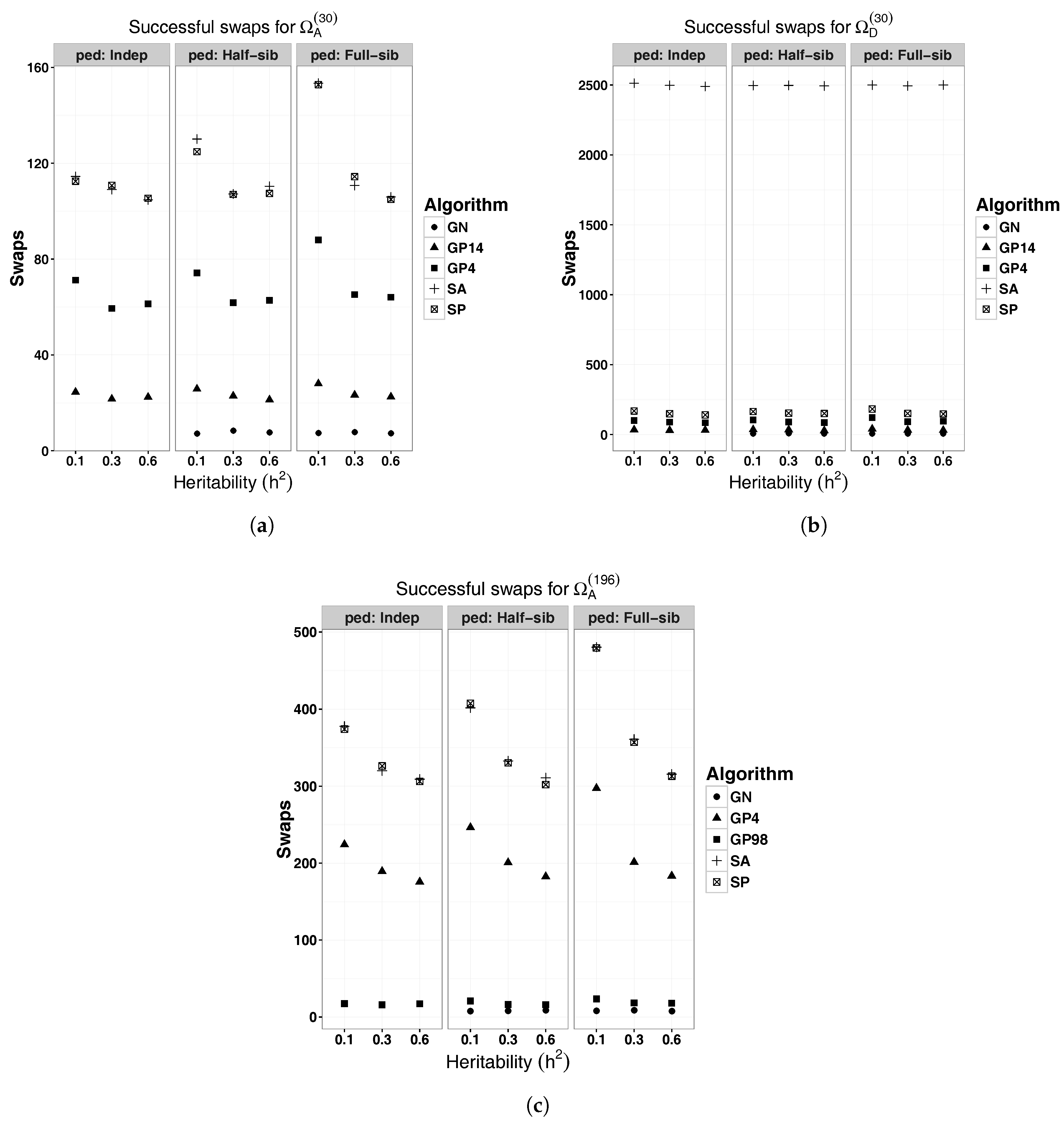
  • Simple Pairwise (SP), that swaps a single pair of treatments at a time,
  • Greedy Pairwise (GP), that swaps more than a single pair of treatments at a time,
  • Genetic Neighbourhood (GN), that takes into consideration the genetic relatedness of the direct neighbouring of a experimental units to perform swaps, and
  • Simulated Annealing (SA), that swaps a pair of treatments at a time, but accepts poor designs at random with a given probability which diminishes with time.
The procedure for these algorithms involves randomly generating m initial experimental layouts, denoted as Ω i . For each layout, the variance–covariance matrix of the treatment effects M ( Ω ) is obtained, and its criterion value is calculated (as trace or determinant (or log(determinant)) with A- and D-optimality, respectively). Next, from the m designs, the “best” experimental layout is selected, where “best” refers to the design with the smallest trace under A-optimality and design with the largest determinant under the D-optimality. After this, an optimization algorithm is applied for p iterations. For all implemented algorithms, the output is a list of objects including the improved experimental layout, a vector with criterion values and iterations of the sequentially accepted (successful) designs, and a vector of all criterion values from all iterations, whether the swap was successful or not. Following is a description of the implemented algorithms.
For the SP algorithm, the following steps are undertaken after selecting the best initial Ω i with criteria value τ i : (1) randomly interchange a single pair of treatments within a randomly selected block to produce a new layout, τ j ; (2) re-calculate a new criterion value τ j ; (3) if τ i > τ j , accept Ω j as the new layout; and (4) repeat steps 1 to 3 for a total of p iterations and produce the output.
GP algorithms are a more aggressive variant of the simple pairwise algorithm (SP) that allow multiple treatments to be randomly interchanged within a block. In order to evaluate a spectrum of alternative implementations, this algorithm was implemented by varying the number of treatments to be swapped simultaneously, denoted as G α , where α refers to the number of treatments swapped. The implemented algorithm allows specification of any even number of treatments to be swapped at a time. Tested procedures were denoted as GP4, GP14 and GP98 for randomly swapping 4, 14 and 98 treatments simultaneously on each iteration within a randomly selected block, respectively. Numbers 14 and 98 were chosen as a percentage (≈50%) of the treatments to be swapped at a time, in an experiment with 30 and 196 treatments, respectively, whereas 4 was chosen as a close value to 2 to detect any small changes in improvement of the design when a single pair or double pairs of treatments are swapped in each iteration. Steps 1 to 4 apply as described under the SP procedure.
The GN algorithm is defined as a method that makes use of genetic relatedness of the eight neighbouring experimental units found in a 3 × 3 matrix using information provided by the numerator relationship matrix ( A ) of the corresponding genotypes. Steps for this algorithm are: (1) randomly generate m initial designs and select the best ( Ω i ) with the smallest trace, τ i ; (2) randomly select a treatment t l from Ω i ; (3) identify the genetic correlation coefficients from the numerator relationship matrix for all experimental units within the nearest neighborhood of τ l ; (4) if there exists a pairwise genetic relationship of 0.25 or higher between τ l and any other treatment τ k for l k within the neighbouring matrix, then replace either one of the treatments with a another treatment that is at a distance of more than a unit (row or column) away; (5) if there are no treatments further than a unit away even though these neighbours are genetically correlated, randomly interchange τ l with τ k ; (6) calculate the new criterion value, τ j , based on the new design layout Ω j ; (7) if τ i > τ j , accept Ω j , otherwise reject Ω j ; and (8) repeat steps 2 to 7 for a total of p iterations. Note that if all the experimental units from a neighbourhood are genetically unrelated, then the SP is applied.
SA is a probabilistic meta-heuristic and stochastic optimization procedure that prevents the search from getting trapped in a local optima by accepting some solutions with a set probability and lowering the temperature with time to make sure that poorer solutions are accepted with lower probabilities [14]. The SA algorithm implemented in this study is described as follows: (1) randomly interchange a pair of treatments within a randomly selected block to produce a new layout, Ω j and re-calculate a criterion value, τ j ; (2) if τ i > τ j , accept Ω j as the new layout with probability 1.0 ; else do the following step, (3) calculate = τ j τ i and set a cooling temperature T c [ i ] = 1 / i , for the i-th iteration, and calculate v = exp / T c [ i ] ; (4) draw a random value u from a uniform distribution, and if u < v accept Ω j ; and (5) repeat steps 1 to 4 for a total of p iterations.
The SA method has two parameters that have to be tuned, i.e., initial temperature and cooling rate. In this study, the initial temperatures are the initial criterion values (that is, traces or determinants) of the initial designs before optimization process. The starting initial temperature was chosen to be the best criterion value among the initial designs. For instance, under the A-optimality criterion, choose a design that has the smallest trace (equivalent to starting temperature) as the main initial design to be optimized further. The cooling rate was viewed as part of step 3 above, and also, it can be viewed as a stopping rule. For example, the stopping rule can be the difference between the current criterion value and the previously calculated value (say, a difference of 0.05) observed for a consecutive number of iterations. The stopping rule for the motivating example was set to be the number of iterations p = 20,000 and for all other illustrations, it was set to p = 5000 interations.

2.3. Evaluation of Algorithms

The above four algorithms were evaluated under varying experimental conditions to assess their effectiveness to improve field designs. Conditions considered include narrow-sense heritabilities, m = 1 initial designs, h 2 , of 0.1, 0.3, and 0.6, where h 2 = σ g 2 / ( σ g 2 + σ e 2 ) ; unrelated individuals (independent), half-sib and full-sib families; and a spatial correlation of ρ = 0.6 . Every combination of conditions was repeated λ = 10 times for p = 5000 iterations. All implementation and evaluation of algorithms was done using the statistical package R [22].
The following scenarios were considered: Ω A ( 30 ) , Ω D ( 30 ) and Ω A ( 196 ) . The first two represent RCB designs with 30 genotypes generated using A- and D-optimality criteria, respectively. In these layouts, the designs had six blocks each of dimensions five rows by six columns. Here, pedigree from half-sib families consisted of five male parents each with six individuals, and full-sib families consisted on a half-diallel with five parents for a total of 10 families each with three individuals. Scenario Ω A ( 196 ) represents an RCB design with 196 genotypes generated using A-optimality criterion with four blocks of dimensions 14 rows by 14 columns per block. Pedigree files for half-sib families had 32 known parents each with six offspring, whereas full-sib families had 30 parents with several half-diallels for a total of 68 families each with approximately three offspring. Note that, GP98 was implemented only for Ω A ( 196 ) scenario to swap 50% of the total genotypes at every single iteration, and GP14 represents swapping about 50% of the genotypes for Ω A ( 30 ) and Ω D ( 30 ) scenarios.
A detailed practical example was implemented with all algorithms in order to investigate the level of design efficiencies and rates of convergence that can be obtained for a specified condition with all algorithms having to improve the same initial RCB experimental design. This was done using A-optimality criterion for an experiment with 30 genotypes, 6 blocks of sizes 5 rows by 6 columns, and comprised of half-sib families with five male parents each with six individuals, for h 2 = 0.1 , ρ = 0.6 , and an arbitrary nugget effect of 0.1. Initially, m = 1000 designs were randomly generated and the best one selected for optimization. All the proposed algorithms were made to improve this initial design by going through p = 20,000 iterations. Traces from both successful and unsuccessful swaps were observed together with the time taken for each algorithm. The practical example was run from a 64-bit windows operating system Intel(R) Core(TM) i7-4720HQ [email protected], RAM 8.0 GB.
To evaluate the improvement of a design, relative overall design efficiency (ODE), that quantifies how efficient the improved design is relative to an initially non-improved design for A- and D-optimality was calculated as a proportion or percentage difference between the initial best criterion and the final optimal-value:
γ i j A = A ¯ i j A ( o p t ) i j A ¯ i j ; γ i j D = D ¯ i j D ( o p t ) i j D ¯ i j ; for i = 1 , 2 , , ξ conditions ; j = 1 , 2 , , λ replicates
where A ¯ i j and D ¯ i j are averages of m initial traces and log-determinants, respectively, for i-th condition and j-th replicate, A ( o p t ) i j and D ( o p t ) i j are the smallest trace and log-determinant, respectively, obtained from an improved design. Finally, ODE calculations over the λ = 10 replicates per condition were summarized. A schematic diagram that represents a summary of the procedure to improve a given randomized complete block design is displayed in Figure 1 and Table 1 shows the simulation conditions implemented for the motivating example.
The R-code that was used for the algorithms described in this paper have been provided in Appendix A. The R-code to generate the initial RCBD before optimization is shown in Appendix B while Appendix C and Appendix D provide the R-code for generating the numerator relationship matrix and the variance–covariance matrix, respectively. Supplementary materials that include additional R-code, a worked-out example using RMarkdown and the pedigree information are also available for illustration purposes.

3. Results

Averages and standard errors (S.E.) of overall design efficiency (ODE %) for the three scenarios, that is, Ω A ( 30 ) , Ω A ( 196 ) and Ω D ( 30 ) for all algorithms are presented in Table 2, Table 3 and Table 4, respectively. Figure 2 displays visible trends of ODEs by genetic relatedness and heritability levels whereas Figure 3 shows the average number of successful swaps out of 5000 (that is, swaps that were accepted due to the resulting design having a smaller criterion value than the previous layout) for each algorithm. These results indicate that, for all experiments conducted based on Ω A ( 30 ) and Ω A ( 196 ) scenarios, simulated annealing (SA) and simple pairwise (SP) algorithms achieved the highest ODE averages in all evaluated conditions followed by GP4 (for Ω A ( 30 ) ) or GP98 (for Ω A ( 196 ) ) and lowest for genetic neighbourhood (GN). Also, the overall highest ODEs were achieved when h 2 = 0.3 among genetically unrelated individuals for all algorithms. Among full-sib families, highest ODEs were achieved when h 2 = 0.1 and decreased with increasing heritability for all algorithms evaluated under Ω A ( 30 ) and Ω A ( 196 ) scenarios. SA recorded the highest average ODE of 7.403 % (S.E. = 0.063) followed by SP with average ODE of 7.398 % (S.E. = 0.066) all obtained when h 2 = 0.3 among genetically unrelated individuals. Algorithms SA, SP, GP4 and GP14 evaluated with half-sib families under Ω A ( 30 ) had highest ODEs obtained for treatments with the lowest heritability of 0.1 , whereas GN achieved its highest ODE when h 2 = 0.3 for the same genetic structure.
Based on a Ω D ( 30 ) scenario, the best performing algorithm with highest average ODE among all conditions was SP, closely followed by GP4, GP14, GN and SA which recorded the lowest average ODE. Under this scenario, the overall highest ODEs were observed among genetically unrelated individuals for SP, GP4, and GP14 when h 2 = 0.3 . Among half-sib families, highest ODEs occurred when h 2 = 0.3 but no clear trends among full-sib families were observed.
Both Ω A ( 30 ) and Ω D ( 30 ) took, on average, about 2 min to improve a given initial experimental design for p = 5000 iterations, whereas Ω A ( 196 ) required about 25 min for the same number of iterations. Figure 3 shows that the number of successful swaps decrease with increasing heritability especially for Ω A ( 30 ) and Ω A ( 196 ) scenarios with small difference in numbers between SA and SP algorithms but larger differences are noted under Ω D ( 30 ) scenario. The number of successful swaps out of 5000 appeared to be highest for SA and SP under A-optimality criterion. From Ω D ( 30 ) scenario, the number of successful swaps were highest for SA which recorded above 2500 out of the 5000 swaps but this was not refelcted in terms of improving the overall design efficiency under this criterion in contrast with other algorithms.
Results from the practical example that was conducted for an RCB design with h 2 = 0.1 and ρ = 0.6 based on Ω A ( 30 ) are displayed in Figure 4 which plots traces obtained from successful swaps and their overall design efficiencies. Also, Figure 5 shows the rate of convergence by plotting all the 20,000 traces obtained for each algorithm. From this illustration, the results indicate that the SP algorithm had the highest design efficiency of 6.713 % with the highest number of successful swaps (192) and took about 5.8 min for the 20,000 iterations. This was closely followed by the SA algorithm that had an ODE of 6.258 % with 139 successful swaps and took about 5.8 min. GP4 algorithm had an ODE of 5.552 % with 104 successful swaps and also took about 5.8 min and finally, the GN algorithm recorded the lowest ODE of 2.053 % with 12 successful swaps and took about 6.1 min.

4. Discussion

Optimization algorithms are commonly used in agriculture and forestry research for several planning and management problems [23,24]. In the current study, an array of these algorithms was implemented and evaluated to assess how well the efficiency of experimental designs can be improved once spatial and genetical correlation is considered. In particular, the evaluation of algorithm efficiency to improve experimental designs focused on the use of RCB designs in field trials with application in plant breeding. Family structure such as half-sib or full-sib families requires appropriate modelling of their genetic relationships (i.e., correlations) and similarly, their phyisical proximity within rows and/or columns needs to be accounted for as genotypes in close range will share microsite and thus will be correlated. Here, accounting for spatial correlations within rows and columns was necessary to minimize this experimental bias. Incorporation of these correlations not only on the desing stage but also in the analysis stage has been shown by Gezan et al. [5], for RCB desgins, to produce designs that are nearly as efficient as those generated using more complex models such as row-column designs that were analyzed assuming uncorrelated residual errors.
From the detailed practical example that examined a specific condition, results indicated that the SP algorithm is the best as it managed to improve the initial experiment by reducing the average variance of treatment effects by 6.713%. This was followed closely by the SA algorithm with an ODE of 6.258%. The more aggressive algorithm GP4, under the evaluated experimental conditions, was underperfoming but it might do better in other design conditions. Also, the algorithm GN had only 12 successful swaps, which was much less than SP and SA algorithms which recorded 192 and 139 swaps, respectively.
Results from Table 2 and Table 3 have shown that SP and SA algorithms achieved the highest relative design efficiencies under all experimental conditions for Ω A ( 30 ) and Ω A ( 196 ) scenarios with the next best algorithm appearing to be the GP4 algorithm followed by GP14 for Ω A ( 30 ) scenario or GP98 for Ω A ( 196 ) scenario, and last by the GN algorithm. These results could be attributable to the fact that SP swaps a single pair of treatments per iteration, thus taking small steps in the search for an optimal design which makes it more likely to find an optimal condition than GP algorithms that take larger random steps. SA algorithm performed well under A-optimality criterion since it has the ability not to be trapped in a local minima by accepting a proportion of bad solutions using an exponential distribution and a cooling schedule. It is expected that this algorithm will have better performance in tha case of hundreds or thousand entries, where the likelihood of being trapped in local minuma is higher. SA algorithm achieved the lowest relative design efficiencies for the same number of iterations of 5,000 under Ω D ( 30 ) scenario as shown in Table 4. It is not very clear why this occurs, but it was observed that it accepted too many bad (or random) solutions as it tried not to be trapped in a local minima, hence, making its progress difficult to maximize the objective function.
This study demonstrated that the incorporation of genetic relationships can affect the optimality of a given design. However, large design improvements have been observed among genetically unrelated individuals, which agrees with findings from Filho and Gilmour [25] although they did not analyse varied levels of spatial correlations. Optimization based on A-criterion has revealed, from the present study, that a substantial decrease in average variance of treatment effects (i.e., trace) among full-sib families can be achieved for treatments with small levels of narrow-sense heritabilities ( h 2 = 0.1 ). For the case of full-sibs with large narrow-sense heritabilities levels such as 0.6 and with a spatial correlation of 0.6 , little improvements on the design efficiencies were noted. For experimental designs that were evaluated under Ω A ( 30 ) scenario, the amount of design improvement was, for some conditions, about four times larger than that realized under Ω A ( 196 ) scenario. This means that more iterations (>50,000) might be required for larger experiments than it would take for a smaller experiment to to reach an adequate optimal solution [10]. The number of successful swaps displayed in Figure 3 indicates that they decrease with increasing heritability for all families for experiments evaluated under Ω A ( 196 ) and Ω A ( 30 ) scenarios for almost all algorithms.
The choice of A- or D-optimality criteria depends on the desired objective function to be minimized. Both criteria are a convex function of eigenvalues [11,13]. Here, A-optimality is a function of the arithmetic mean of the eigenvalues of this matrix whereas D-optimality is a function of the geometric mean of these eigenvalues [11]. It is recommended to favor the use of the A-optimality criterion, given the additional computational time required to calculated the determinant within the D-optimality, particularly for large experiments such as the Ω A ( 196 ) scenarios. If additional approximations to the procedures are required to accelerate the optimization process, then a similar approach to the one described by Butler et al. [26] can be implemented.
The algorithms and procedures presented in this study can be easily extended to other complex experimental designs such as non-orthogonal experiments that can be implemented with appropriate extensions of the linear mixed models together with an optimality criterion of choice. In addition, other variants of the search algorithms can also be used; for instance, for the GN algorithm a value different from 0.25 could be chosen to determine when, and which, treatments should be swapped. It was not evaluated if changing this threshold value would increase the efficiency of the GN algorithm.
In summary, the potential to improve experimental designs such as RCB designs has been shown in this study to be highest when SP and SA algorithms were used under A-optimality criterion. For both A- and D-optimality criteria, SP presented the highest overall design efficiencies. In conclusion, the use of a SP algorithm based on A-optimality criterion, under a linear mixed model framework that incorporates genetic relatedness and/or spatial correlations is promising. The procedure enables generation of more efficient field designs (by reducing the average variance of the treatment effects) to be used in operational plant breeding programs or in other design of experiments.

Supplementary Materials

The following are available online at https://www.mdpi.com/1999-4893/11/12/212/s1, Examples.pdf, ped30hs.csv, ped30fs.csv, ped196HS.csv, ped196FS.csv, and final.R.

Author Contributions

L.K.M. and S.A.G. conceived and designed the experiments and wrote the paper; L.K.M. performed the experiments and analyzed the data.

Funding

This research received no external funding.

Acknowledgments

The authors would like to thank the University of Florida’s Institute of Food and Agricultural Sciences (UF/IFAS) for funding the study as part of a Ph.D. thesis for Mramba.

Conflicts of Interest

The authors declare no conflict of interest.

Appendix A. R-Code for the Algorithms

Appendix A.1. Simple Pairwise Algorithm (SP)

Algorithms 11 00212 i001
Algorithms 11 00212 i002

Appendix A.2. Simulated Annealing Algorithm (SA)

Algorithms 11 00212 i003
Algorithms 11 00212 i004

Appendix A.3. Greedy Pairwise Algorithm (GP)

Algorithms 11 00212 i005
Algorithms 11 00212 i006

Appendix A.4. Genetic Neighborhood Algorithm (GN)

Algorithms 11 00212 i007
Algorithms 11 00212 i008

Appendix B. R-Code for Generating Initial Randomized Complete Block Design (RCBD)

Appendix B.1. Generate a RCBD

Algorithms 11 00212 i009
Algorithms 11 00212 i010

Appendix B.2. Generate Multiple RCBD

Algorithms 11 00212 i011

Appendix C. Generate a Numerator Relationship Matrix

Algorithms 11 00212 i012Algorithms 11 00212 i013

Appendix D. Calculate the Variance-Covariance Matrix

Algorithms 11 00212 i014Algorithms 11 00212 i015

References

  1. Welham, S.J.; Gezan, S.A.; Clark, S.J.; Mead, A. Statistical Methods in Biology; Design and Analysis of Experiments and Regression; Chapman & Hall: Boca Raton, FL, USA, 2015. [Google Scholar]
  2. Piepho, H.P.; Möhring, J.; Melchinger, A.E.; Büchse, A. BLUP for phenotypic selection in plant breeding and variety testing. Euphytica 2008, 161, 209–228. [Google Scholar] [CrossRef]
  3. John, J.A.; Williams, E.R. Cyclic and Computer Generated Designs, 2nd ed.; Monographs of Statistics and Applied Probability 38; Chapman and Hall: London, UK, 1995. [Google Scholar]
  4. Williams, E.R.; John, J.A.; Whitaker, D. Construction of resolvable spatial row-column designs. Biometrics 2006, 62, 103–108. [Google Scholar] [CrossRef] [PubMed]
  5. Gezan, S.A.; White, T.L.; Huber, D.A. Accounting for spatial variability in breeding trials: A simulation study. Agronomy 2010, 102, 1562–1571. [Google Scholar] [CrossRef]
  6. Butler, D.G.; Smith, A.B.; Cullis, B.R. On the design of field experiments with correlated treatment effects. J. Agric. Biol. Environ. Stat. 2014, 19, 539–555. [Google Scholar] [CrossRef]
  7. Chernoff, H. Locally optimal designs for estimating parameters. Ann. Math. Stat. 1953, 24, 586–602. [Google Scholar] [CrossRef]
  8. Cullis, B.R.; Lill, W.; Fisher, J.; Read, B.; Gleeson, A. A new procedure for the analysis of early generation variety trials. J. R. Stat. Soc. Ser. C (Appl. Stat.) 1989, 38, 361–375. [Google Scholar] [CrossRef]
  9. Cullis, B.R.; Smith, A.B.; Coombes, N.E. On the design of early generation variety trials with correlated data. J. Agric. Biol. Environ. Stat. 2006, 11, 381–393. [Google Scholar] [CrossRef]
  10. Mramba, L.K.; Peter, G.F.; Whitaker, V.M.; Gezan, S.A. Generating improved experimental designs with spatially and genetically correlated observations using mixed models. Agronomy 2018, 8, 40. [Google Scholar] [CrossRef]
  11. Kuhfeld, W.F. MR-2010C—Experimental Design: Efficiency, Coding, and Choice Designs; Technical Report; SAS Insitute Inc.: Cary, NC, USA, 2010. [Google Scholar]
  12. Wald, A. On the efficient design of statistical investigations. Ann. Math. Stat. 1943, 14, 134–140. [Google Scholar] [CrossRef]
  13. Das, A. An introduction to optimality criteria and some results on optimal block design. In Design Workshop Lecture Notes; Indian Statistical Institute: Kolkata, India; Theoretical Statistics and Mathematics Unit: New Delhi, India, 2002; pp. 1–21. [Google Scholar]
  14. Kirkpatrick, S.; Gelatt, C.; Vecchi, M.P. Optimization by simulated annealing. Science 1983, 220, 671–680. [Google Scholar] [CrossRef] [PubMed]
  15. VSN International. CycDesign 6.0: A Package for the Computer Generation of Experimental Designs; VSN International Ltd.: Hemel Hempstead, UK, 2018. [Google Scholar]
  16. VSN International. Genstat for Windows, 19th ed.; VSN International Ltd.: Hemel Hempstead, UK, 2017. [Google Scholar]
  17. Coombes, N.E. DiGGer: Design Search Tool in R. 2009. Available online: http://nswdpibiom.org/austatgen/software/ (accessed on 17 December 2018).
  18. Cressie, N.A.C. Statistics for Spatial Data, revised ed.; John Wiley & Sons, Inc.: New York, NY, USA, 1993. [Google Scholar]
  19. Gilmour, A.R.; Gogel, B.J.; Cullis, B.R.; Thompson, R. ASReml User Guide Release 3.0; VSN International Ltd.: Hemel Hempstead, UK, 2009. [Google Scholar]
  20. Henderson, C.R. The estimation of genetic parameters. Ann. Math. Stat. 1950, 21, 309–310. [Google Scholar]
  21. Hooks, T.; Marx, D.; Kachman, S.; Pedersen, J. Optimality criteria for models with random effects. Revista Colombiana de Estadística 2009, 32, 17–31. [Google Scholar]
  22. R Core Team. R: A Language and Environment for Statistical Computing; R Foundation for Statistical Computing: Vienna, Austria, 2018. [Google Scholar]
  23. Borges, P.; Eid, T.; Bergseng, E. Applying simulated annealing using different methods for the neighborhood search in forest planning problems. Eur. J. Oper. Res. 2014, 233, 700–710. [Google Scholar] [CrossRef]
  24. Liu, G.; Han, S.; Zhao, X.; Nelson, J.D.; Wang, H.; Wang, W. Optimisation algorithms for spatially constrained forest planning. Ecol. Model. 2006, 194, 421–428. [Google Scholar] [CrossRef]
  25. Filho, J.S.B.; Gilmour, S.G. Planning incomplete block experiments when treatments are genetically related. Biometrics 2003, 59, 375–381. [Google Scholar] [CrossRef]
  26. Butler, D.G.; Eccleston, J.A.; Cullis, B.R. On an approximate optimality criterion for the design of field experiments under spatial dependence. Aust. N. Z. J. Stat. 2008, 50, 295–307. [Google Scholar] [CrossRef]
Figure 1. Schematic diagram to summarize the procedure for improving a randomized complete block (RCB) design.
Algorithms 11 00212 g001
Figure 2. Overall design efficiency (ODE %) for (a) Ω A ( 30 ) , (b) Ω D ( 30 ) , and (c) Ω A ( 196 ) scenarios evaluated for simple pairwise (SP), greedy pairwise (GP4, GP14, GP98), simulated annealing (SA) and genetic neighborhood (GN) algorithms iterated p = 5000 times, with each condition replicated λ = 10 times, with m = 100 initially unimproved designs.
Algorithms 11 00212 g002
Figure 3. Average number of swaps for (a) Ω A ( 30 ) , (b) Ω D ( 30 ) , and (c) Ω A ( 196 ) scenarios evaluated for simple pairwise (SP), greedy pairwise: GP4, GP14, GP98, simulated annealing (SA) and genetic neighborhood (GN) algorithms iterated p = 5000 times, with each condition replicated λ = 10 times, with m = 100 initially unimproved designs.
Algorithms 11 00212 g003
Figure 4. Traces from successful swaps to convey the rate of convergence for simple pairwise (SP), simulated annealing (SA), greedy pairwise (GP4), and genetic neighborhood (GN) algorithms with their overall design efficiencies (ODE) evaluated for half-sib families with h 2 = 0.1 , ρ = 0.6 and a nugget error of 0.1 iterated for 20,000 for a practical Ω A ( 30 ) example.
Algorithms 11 00212 g004
Figure 5. Rates of convergence for (a) simple pairwise (SP), (b) simulated annealing (SA), (c) greedy pairwise (GP4), and (d) genetic neighborhood (GN) showing all traces obtained from these algorithms evaluated for half-sib families with h 2 = 0.1 , ρ = 0.6 and a nugget error of 0.1 iterated for 20,000 for a practical Ω A ( 30 ) example.
Algorithms 11 00212 g005
Table 1. Simulation conditions for the motivating example assuming a spatial correlation ρ = 0.6 and a nugget error of 0.1 for the three designs: Ω A ( 30 ) , Ω A ( 196 ) and Ω D ( 30 ) , where Ω A ( 30 ) represents an RCB design with 30 treatments (genotypes) arranged in 6 blocks of sizes 5 rows by 6 columns and optimized using an A-optimality criterion. Initial m = 1000 designs were generated and the overall best design (design with smallest trace under A-optimality or largest determinant under D-optimality) selected to be optimized. The algorithm was stopped after p = 20,000 iterations. Final designs for each condition represented the improved design and the ODE % are calculated using Equations (1) and (2). Each of the nine conditions was repeated λ = 10 times for all four algorithms: SP, GP4, GP14 and SA.
Condition h 2 Pedigree
10.1Indep
20.3
30.6
40.1Half-sib
50.3
60.6
70.1Full-sib
80.3
90.6
Table 2. Average ODEs from 10 replicates per condition are reported together with standard errors (S.E.) for simple pairwise (SP), greedy pairwise (GP4 and GP14), simulated annealing (SA) and genetic neighborhood (GN) procedures for Ω A ( 30 ) RCB designs at a spatial correlation of 0.6 .
Condition SP GP4 GP14 SA GN
Pedigree h 2 ODE %S.E. ODE %S.E. ODE %S.E. ODE %S.E. ODE %S.E
Indep0.1 6.3470.060 5.5010.060 3.7470.093 6.3850.072 --
0.3 7.3980.066 6.1940.080 4.3710.053 7.4030.063 --
0.6 5.1090.044 4.4140.057 3.1100.054 5.2220.064 --
Half-sib0.1 5.8260.026 5.0820.055 3.6100.065 5.7810.045 1.8530.042
0.3 5.3750.056 4.6400.082 3.1920.052 5.4280.047 1.9400.088
0.6 3.0660.028 2.6630.023 1.8580.033 3.1310.028 1.0640.033
Full-sib0.1 4.1090.030 3.6110.026 2.5430.038 4.0450.027 1.3430.034
0.3 2.6560.029 2.2650.021 1.6010.034 2.6670.032 0.9200.027
0.6 1.2470.006 1.0650.009 0.7550.012 1.2470.013 0.4600.011
Table 3. Average ODEs reported together with standard errors (S.E.) for simple pairwise (SP), greedy pairwise (GP4 and GP98), simulated annealing (SA) and genetic neighborhood (GN) procedures for Ω A ( 196 ) RCB designs at a spatial correlation of 0.6 .
Condition SP GP4 GP98 SA GN
Pedigree h 2 ODE %S.E. ODE %S.E. ODE %S.E. ODE %S.E. ODE %S.E
Indep0.1 1.6330.013 1.3540.018 0.4810.008 1.6290.015 --
0.3 2.7940.020 2.3870.017 0.8640.024 2.7360.034 --
0.6 3.2320.024 2.7540.039 1.0800.028 3.2700.027 --
Half-sib0.1 2.0320.023 1.7760.019 0.6900.018 2.0160.019 0.2160.014
0.3 2.6840.018 2.2690.009 0.8510.024 2.6700.019 0.3810.013
0.6 2.8010.027 2.4020.029 0.8900.025 2.8180.009 0.3510.020
Full-sib0.1 2.8130.018 2.4710.022 0.8880.025 2.8270.014 0.3240.015
0.3 2.2400.016 1.8860.023 0.7020.020 2.2260.021 0.2970.011
0.6 1.8730.011 1.5880.013 0.6230.016 1.9260.013 0.2800.013
Table 4. Average ODEs reported together with standard errors (S.E.) for simple pairwise (SP), greedy pairwise (GP4 and GP14), simulated annealing (SA) and genetic neighborhood (GN) procedures for Ω D ( 30 ) RCB designs at a spatial correlation of 0.6 .
Condition SP GP4 GP14 SA GN
Pedigree h 2 ODE %S.E. ODE %S.E. ODE %S.E. ODE %S.E. ODE %S.E
Indep0.1 1.8070.014 1.6000.014 1.0290.014 0.0850.019 --
0.3 2.3240.017 1.9930.013 1.3350.030 0.1040.025 --
0.6 2.2470.021 1.9300.021 1.2650.032 0.1780.027 --
Half-sib0.1 1.7660.012 1.5760.015 1.1150.015 0.1300.034 0.4460.015
0.3 2.2870.023 2.0540.024 1.3770.022 0.1500.041 0.6140.013
0.6 2.2530.024 1.9330.020 1.3150.019 0.0900.023 0.6370.023
Full-sib0.1 1.6660.011 1.5140.013 1.0370.009 0.0970.025 0.4310.010
0.3 2.1680.013 1.9350.025 1.3070.026 0.1190.025 0.6340.017
0.6 2.2250.027 1.9130.023 1.3160.025 0.1250.019 0.6690.022

