A Connection Between the Kalman Filter and an Optimized LMS Algorithm for Bilinear Forms

Abstract

The system identification problem becomes more challenging when the parameter space increases. Recently, several works have focused on the identification of bilinear forms, which are related to the impulse responses of a spatiotemporal model, in the context of a multiple-input/single-output system. In this framework, the problem was addressed in terms of the Wiener filter and different basic adaptive algorithms. This paper studies two types of algorithms tailored for the identification of such bilinear forms, i.e., the Kalman filter (along with its simplified version) and an optimized least-mean-square (LMS) algorithm. Also, a comparison between them is performed, which shows interesting similarities. In addition to the mathematical derivation of the algorithms, we also provide extensive experimental results, which support the theoretical findings and indicate the good performance of the proposed solutions.

1. Introduction

Bilinear systems were previously treated in various contexts [1], such as the nonlinear systems approximation. The applications derived from there are numerous, among which we can mention system identification [2,3,4,5], design of digital filters [6], echo cancellation [7], chaotic communications [8], active noise control [9], neural networks [10], etc. In all these papers, the bilinear term is understood in terms of an input-output relation (with respect to the data).

More recently, a new approach was studied in [11], where the bilinear term was defined in the context of a multiple-input/single-output (MISO) system, with respect to the impulse responses of a spatiotemporal model. In [11], the Wiener filter solution for the identification of such bilinear forms was proposed, and then, in [12,13,14], some adaptive solutions based on different basic algorithms were provided. Similar frameworks can be found in [15,16,17,18], in conjunction with specific applications, such as channel equalization and nonlinear acoustic echo cancellation; however, these works were not associated with the identification of bilinear forms or analyzed in this context.

The Kalman filter was first introduced in [19] and it has a wide range of applications in technology, as well as in signal processing [20]. Some of its applications in the automotive field are mentioned in [21,22], and the references therein, while [23] also provides a computational complexity analysis.

In this paper, we focus on a comparative study of two different types of algorithms tailored for the identification of bilinear forms. The first one is based on the Kalman filter [19], whose bilinear form was introduced in our previous work [13], together with a simplified (i.e., low complexity) version, which could be more suitable in real-world applications. The second algorithm is a version of the least-mean-square (LMS) adaptive filter, but where the step-size parameter has been optimized in order to meet a proper compromise between the convergence rate and misadjustment. In addition, as it will be shown, there is a strong similarity between the simplified Kalman filter and the optimized LMS algorithm. Simulations show the good performance of the proposed solutions, in comparison with other related works based on the conventional algorithms. Moreover, the gain could be twofold, in terms of both convergence performance and computational complexity.

The paper structure is as follows. Section 2 introduces the system model in the context of bilinear forms. In this framework, we present the Kalman filter together with its simplified version in Section 3. The optimized LMS algorithm is derived in Section 4. Next, a comparison between the simplified Kalman filter and the optimized LMS algorithm for bilinear forms is presented in Section 5. Section 6 provides some practical considerations. Simulations are performed in the framework of system identification and the results are given in Section 7. Finally, some conclusions are drawn in Section 8. Also, Appendix A provides detailed computations of some terms required within the optimized LMS algorithm, while Appendix B summarizes and briefly explains the main parameters used in the paper, in order to facilitate the reading. For the sake of clarity, the main notation used in this work is provided in

Table 1. Notation used throughout the paper.

Symbol	Significance
a	scalar a
$\mathbf{a}$	vector $\mathbf{a}$
$\mathbf{A}$	matrix $\mathbf{A}$
${}^T$	transpose operator
⊗	Kronecker product operator
$\parallel \mathbf{b}\parallel$	Euclidean norm of the vector $\mathbf{b}$
$\mathbb{E}(·)$	mathematical expectation
${\mathbf{I}}_L$	identity matrix of size $L\times L$
$\mathrm{tr}\left(\mathbf{B}\right)$	trace of the square matrix $\mathbf{B}$
$\mathrm{vec}\left(\mathbf{C}\right)=\mathbf{c}$	vectorization operation, i.e., conversion of a matrix ($\mathbf{C}$ of size $L\times M$) into a vector ($\mathbf{c}$ of length $ML$)

.

2. System Model

The signal model that shall be used throughout the paper is given by [11]

$$\begin{array}{cc}\hfill d\left(n\right)& ={\mathbf{h}}^T\left(n\right)\mathbf{X}\left(n\right)\mathbf{g}\left(n\right)+v\left(n\right)\hfill \\ \hfill & =y\left(n\right)+v\left(n\right),\hfill \end{array}$$

(1)

where $d\left(n\right)$ is the zero-mean desired (or reference) signal at the discrete-time index n, $\mathbf{h}\left(n\right)$ and $\mathbf{g}\left(n\right)$ are the two impulse responses of the system of lengths L and M, respectively, the superscript ${}^T$ is the transpose operator, $\mathbf{X}\left(n\right)=[{\mathbf{x}}_1\left(n\right){\mathbf{x}}_2\left(n\right)\dots {\mathbf{x}}_M\left(n\right)]$ is the zero-mean multiple-input signal matrix, ${\mathbf{x}}_m\left(n\right)={[x_m\left(n\right)x_m(n-1)\dots x_m(t-L+1)]}^T$ is a vector containing the L most recent time samples of the mth ($m=1,2,\dots ,M$) input signal, $y\left(n\right)={\mathbf{h}}^T\left(n\right)\mathbf{X}\left(n\right)\mathbf{g}\left(n\right)$ is the output signal and it represents a bilinear form, and $v\left(n\right)$ is a zero-mean additive noise (with the variance ${\sigma }_v^2$). It is assumed that all signals are real-valued, and $\mathbf{X}\left(n\right)$ and $v\left(n\right)$ are independent. As we can notice, $y\left(n\right)$ is a bilinear function of $\mathbf{h}\left(n\right)$ and $\mathbf{g}\left(n\right)$, because for every fixed $\mathbf{h}\left(n\right)$, $y\left(n\right)$ is a linear function of $\mathbf{g}\left(n\right)$, and for every fixed $\mathbf{g}\left(n\right)$, it is a linear function of $\mathbf{h}\left(n\right)$.

We can rewrite the matrix $\mathbf{X}\left(n\right)$, of size $L\times M$, as a vector of length $ML$, by using the vectorization operation:

$$\mathrm{vec}\left[\mathbf{X}\left(n\right)\right]={[{\mathbf{x}}_1^T\left(n\right){\mathbf{x}}_2^T\left(n\right)\dots {\mathbf{x}}_M^T\left(n\right)]}^T=\tilde{\mathbf{x}}\left(n\right).$$

(2)

Therefore, the output signal can be expressed as

$$\begin{array}{cc}\hfill y\left(n\right)& ={\mathbf{h}}^T\left(n\right)\mathbf{X}\left(n\right)\mathbf{g}\left(n\right)\hfill \\ \hfill & ={\left[\mathbf{g}\left(n\right)\otimes \mathbf{h}\left(n\right)\right]}^T\tilde{\mathbf{x}}\left(n\right)={\mathbf{f}}^T\left(n\right)\tilde{\mathbf{x}}\left(n\right),\hfill \end{array}$$

(3)

where ⊗ denotes the Kronecker product between the individual impulse responses, while the vector $\mathbf{f}\left(n\right)=\mathbf{g}\left(n\right)\otimes \mathbf{h}\left(n\right)$, of length $ML$, represents the spatiotemporal (i.e., global) impulse response of the system. Consequently, the signal model in (1) becomes

$$d\left(n\right)={\mathbf{f}}^T\left(n\right)\tilde{\mathbf{x}}\left(n\right)+v\left(n\right).$$

(4)

The major difference compared to a general MISO system is yielded by the fact that in this bilinear context $\mathbf{f}\left(n\right)$ is formed with only $M+L$ different elements, despite being of length $ML$.

The goal is the identification of the two impulse responses $\mathbf{h}\left(n\right)$ and $\mathbf{g}\left(n\right)$, and, in this way, of the spatiotemporal impulse response $\mathbf{f}\left(n\right)$. For this aim, we can use two adaptive filters, $\widehat{\mathbf{h}}\left(n\right)$ and $\widehat{\mathbf{g}}\left(n\right)$; hence, the global impulse response can be evaluated as

$$\widehat{\mathbf{f}}\left(n\right)=\widehat{\mathbf{g}}\left(n\right)\otimes \widehat{\mathbf{h}}\left(n\right).$$

(5)

Let $\eta \ne 0$ be a real-valued constant. We can see from (1) that

$$\left[\frac{1}{\eta }{\mathbf{h}}^T\left(n\right)\right]\mathbf{X}\left(n\right)\left[\eta \mathbf{g}\left(n\right)\right]={\mathbf{h}}^T\left(n\right)\mathbf{X}\left(n\right)\mathbf{g}\left(n\right)=y\left(n\right),$$

(6)

meaning that the pairs $\left[\mathbf{h}\left(n\right)/\eta ,\eta \mathbf{g}\left(n\right)\right]$ and $\left[\mathbf{h}\left(n\right),\mathbf{g}\left(n\right)\right]$ are equivalent in the bilinear form. This implies that we can only identify $\widehat{\mathbf{h}}\left(n\right)$ and $\widehat{\mathbf{g}}\left(n\right)$ up to a scaling factor. A similar discussion can be found in [15,18] in the framework of blind identification/equalization and nonlinear acoustic echo cancellation, respectively. Nevertheless, because

$$\mathbf{f}\left(n\right)=\mathbf{g}\left(n\right)\otimes \mathbf{h}\left(n\right)=\left[\eta \mathbf{g}\left(n\right)\right]\otimes \left[\frac{1}{\eta }\mathbf{h}\left(n\right)\right],$$

(7)

the global impulse response can be identified with no scaling ambiguity. Consequently, for the performance evaluation of the identification of the temporal and spatial filters, we can use the normalized projection misalignment (NPM), defined in [24]:

$$\begin{array}{cc}\hfill \mathrm{NPM}\left[\mathbf{h}\left(n\right),\widehat{\mathbf{h}}\left(n\right)\right]& =1-{\left[\frac{{\mathbf{h}}^T\left(n\right)\widehat{\mathbf{h}}\left(n\right)}{\parallel \mathbf{h}\left(n\right)\parallel \parallel \widehat{\mathbf{h}}\left(n\right)\parallel }\right]}^2,\hfill \end{array}$$

(8)

$$\begin{array}{cc}\hfill \mathrm{NPM}\left[\mathbf{g}\left(n\right),\widehat{\mathbf{g}}\left(n\right)\right]& =1-{\left[\frac{{\mathbf{g}}^T\left(n\right)\widehat{\mathbf{g}}\left(n\right)}{\parallel \mathbf{g}\left(n\right)\parallel \parallel \widehat{\mathbf{g}}\left(n\right)\parallel }\right]}^2,\hfill \end{array}$$

(9)

where $\parallel ·\parallel$ denotes the Euclidean norm. On the other hand, for the identification of the global filter, $\mathbf{f}\left(n\right)$, we should use the normalized misalignment:

$$\mathrm{NM}\left[\mathbf{f}\left(n\right),\widehat{\mathbf{f}}\left(n\right)\right]=\frac{\parallel \mathbf{f}\left(n\right)-\widehat{\mathbf{f}}{\left(n\right)\parallel }^2}{{\parallel \mathbf{f}\left(n\right)\parallel }^2}.$$

(10)

In [11], this bilinear system identification problem has been studied in terms of the Wiener filter. Therefore, the assumption was that the two impulse responses that need to be identified are time-invariant (which represents a basic assumption in the context of the Wiener filter). In practice, however, these systems could vary in time. For this reason, in this paper, we approach the system identification problem considering that the systems that need to be identified vary in time. Thus, we assume that $\mathbf{h}\left(n\right)$ and $\mathbf{g}\left(n\right)$ are zero-mean random vectors, following a simplified first-order Markov model, i.e.,

$$\begin{array}{cc}\hfill \mathbf{h}\left(n\right)& =\mathbf{h}(n-1)+{\mathbf{w}}_{\mathbf{h}}\left(n\right),\hfill \end{array}$$

(11)

$$\begin{array}{cc}\hfill \mathbf{g}\left(n\right)& =\mathbf{g}(n-1)+{\mathbf{w}}_{\mathbf{g}}\left(n\right),\hfill \end{array}$$

(12)

where ${\mathbf{w}}_{\mathbf{h}}\left(n\right)$ and ${\mathbf{w}}_{\mathbf{g}}\left(n\right)$ are zero-mean white Gaussian noise vectors, with correlation matrices ${\mathbf{R}}_{{\mathbf{w}}_{\mathbf{h}}}\left(n\right)={\sigma }_{w_{\mathbf{h}}}^2{\mathbf{I}}_L$ and ${\mathbf{R}}_{{\mathbf{w}}_{\mathbf{g}}}\left(n\right)={\sigma }_{w_{\mathbf{g}}}^2{\mathbf{I}}_M$, respectively (with ${\mathbf{I}}_L$ and ${\mathbf{I}}_M$ being the identity matrices of sizes $L\times L$ and $M\times M$, respectively). It is considered that ${\mathbf{w}}_{\mathbf{h}}\left(n\right)$ is uncorrelated with $\mathbf{h}(n-1)$ and $v\left(n\right)$, while ${\mathbf{w}}_{\mathbf{g}}\left(n\right)$ is uncorrelated with $\mathbf{g}(n-1)$ and $v\left(n\right)$. The variances ${\sigma }_{w_{\mathbf{h}}}^2$ and ${\sigma }_{w_{\mathbf{g}}}^2$ capture the uncertainties in $\mathbf{h}\left(n\right)$ and $\mathbf{g}\left(n\right)$, respectively.

3. Kalman Filter for Bilinear Forms

In this section, we address the previously described system identification problem in terms of the Kalman filter, summarizing the findings from [13]. In this context, the signal model from (1) may be interpreted as the observation equation, while the system impulse responses can be considered as state equations. Given the two adaptive filters $\widehat{\mathbf{h}}\left(n\right)$ and $\widehat{\mathbf{g}}\left(n\right)$, the estimated signal is given by

$$\widehat{y}\left(n\right)={\widehat{\mathbf{h}}}^T(n-1)\mathbf{X}\left(n\right)\widehat{\mathbf{g}}(n-1).$$

(13)

As a result, the a priori error signal between the desired and estimated signals can be defined as

$$\begin{array}{cc}\hfill e\left(n\right)& =d\left(n\right)-\widehat{y}\left(n\right)\hfill \\ \hfill & =d\left(n\right)-{\widehat{\mathbf{h}}}^T(n-1)\mathbf{X}\left(n\right)\widehat{\mathbf{g}}(n-1)\hfill \\ \hfill & =d\left(n\right)-{\left[\widehat{\mathbf{g}}(n-1)\otimes \widehat{\mathbf{h}}(n-1)\right]}^T\tilde{\mathbf{x}}\left(n\right)\hfill \\ \hfill & =d\left(n\right)-{\widehat{\mathbf{f}}}^T(n-1)\tilde{\mathbf{x}}\left(n\right)\hfill \\ \hfill & =d\left(n\right)-{\widehat{\mathbf{h}}}^T(n-1){\mathbf{x}}_{\widehat{\mathbf{g}}}\left(n\right)\hfill \\ \hfill & =d\left(n\right)-{\widehat{\mathbf{g}}}^T(n-1){\mathbf{x}}_{\widehat{\mathbf{h}}}\left(n\right),\hfill \end{array}$$

(14)

where

$${\mathbf{x}}_{\widehat{\mathbf{g}}}\left(n\right)={[\widehat{\mathbf{g}}(n-1)\otimes {\mathbf{I}}_L]}^T\tilde{\mathbf{x}}\left(n\right),$$

(15)

$${\mathbf{x}}_{\widehat{\mathbf{h}}}\left(n\right)={[{\mathbf{I}}_M\otimes \widehat{\mathbf{h}}(n-1)]}^T\tilde{\mathbf{x}}\left(n\right).$$

(16)

In the context of the linear sequential Bayesian approach, the optimal estimates of the state vectors have the forms [25]:

$$\begin{array}{cc}\hfill \widehat{\mathbf{h}}\left(n\right)& =\widehat{\mathbf{h}}(n-1)+{\mathbf{k}}_{\mathbf{h}}\left(n\right)e\left(n\right),\hfill \end{array}$$

(17)

$$\begin{array}{cc}\hfill \widehat{\mathbf{g}}\left(n\right)& =\widehat{\mathbf{g}}(n-1)+{\mathbf{k}}_{\mathbf{g}}\left(n\right)e\left(n\right),\hfill \end{array}$$

(18)

where ${\mathbf{k}}_{\mathbf{h}}\left(n\right)$ and ${\mathbf{k}}_{\mathbf{g}}\left(n\right)$ are the Kalman gain vectors. Next, we can define the a posteriori misalignments (which represent the state estimation errors) related to the temporal and spatial impulse responses:

$${\mathbf{c}}_{\mathbf{h}}\left(n\right)=\frac{1}{\eta }\mathbf{h}\left(n\right)-\widehat{\mathbf{h}}\left(n\right),$$

(19)

$${\mathbf{c}}_{\mathbf{g}}\left(n\right)=\eta \mathbf{g}\left(n\right)-\widehat{\mathbf{g}}\left(n\right),$$

(20)

for which their correlation matrices are ${\mathbf{R}}_{{\mathbf{c}}_{\mathbf{h}}}\left(n\right)=\mathbb{E}\left[{\mathbf{c}}_{\mathbf{h}}\left(n\right){\mathbf{c}}_{\mathbf{h}}^T\left(n\right)\right]$ and ${\mathbf{R}}_{{\mathbf{c}}_{\mathbf{g}}}\left(n\right)=\mathbb{E}\left[{\mathbf{c}}_{\mathbf{g}}\left(n\right){\mathbf{c}}_{\mathbf{g}}^T\left(n\right)\right]$, respectively, where $\mathbb{E}[·]$ denotes mathematical expectation. As mentioned in Section 2, we can only identify the impulse responses up to this arbitrary scaling factor $\eta$; however, the pair $\mathbf{h}\left(n\right)/\eta$ and $\eta \mathbf{g}\left(n\right)$ is equivalent to the pair $\mathbf{h}$ and $\mathbf{g}$ in the bilinear form. Let us also define the a priori misalignments related to the two impulse responses:

$$\begin{array}{cc}\hfill {\mathbf{c}}_{{\mathbf{h}}_{\mathrm{a}}}\left(n\right)& =\frac{1}{\eta }\mathbf{h}\left(n\right)-\widehat{\mathbf{h}}(n-1)\hfill \\ \hfill & ={\mathbf{c}}_{\mathbf{h}}(n-1)+\frac{1}{\eta }{\mathbf{w}}_{\mathbf{h}}\left(n\right),\hfill \end{array}$$

(21)

$$\begin{array}{cc}\hfill {\mathbf{c}}_{{\mathbf{g}}_{\mathrm{a}}}\left(n\right)& =\eta \mathbf{g}\left(n\right)-\widehat{\mathbf{g}}(n-1)\hfill \\ \hfill & ={\mathbf{c}}_{\mathbf{g}}(n-1)+\eta {\mathbf{w}}_{\mathbf{g}}\left(n\right),\hfill \end{array}$$

(22)

whose correlation matrices are ${\mathbf{R}}_{{\mathbf{c}}_{{\mathbf{h}}_{\mathrm{a}}}}\left(n\right)=\mathbb{E}\left[{\mathbf{c}}_{{\mathbf{h}}_{\mathrm{a}}}\left(n\right){\mathbf{c}}_{{\mathbf{h}}_{\mathrm{a}}}^T\left(n\right)\right]$ and ${\mathbf{R}}_{{\mathbf{c}}_{{\mathbf{g}}_{\mathrm{a}}}}\left(n\right)=\mathbb{E}\left[{\mathbf{c}}_{{\mathbf{g}}_{\mathrm{a}}}\left(n\right){\mathbf{c}}_{{\mathbf{g}}_{\mathrm{a}}}^T\left(n\right)\right]$, respectively.

For the sake of simplicity of the upcoming developments, let us multiply ${\mathbf{w}}_{\mathbf{h}}\left(n\right)$ and ${\mathbf{w}}_{\mathbf{g}}\left(n\right)$ by $1/\eta$ and $\eta$, respectively, and introduce the notation:

$$\begin{array}{cc}\hfill {\overline{\mathbf{w}}}_{\mathbf{h}}\left(n\right)& =\frac{1}{\eta }{\mathbf{w}}_{\mathbf{h}}\left(n\right),\hfill \end{array}$$

(23)

$$\begin{array}{cc}\hfill {\overline{\mathbf{w}}}_{\mathbf{g}}\left(n\right)& =\eta {\mathbf{w}}_{\mathbf{g}}\left(n\right).\hfill \end{array}$$

(24)

These new terms are also zero-mean white Gaussian noise vectors, having the correlation matrices ${\mathbf{R}}_{{\overline{\mathbf{w}}}_{\mathbf{h}}}\left(n\right)={\sigma }_{{\overline{w}}_{\mathbf{h}}}^2{\mathbf{I}}_L$ and ${\mathbf{R}}_{{\overline{\mathbf{w}}}_{\mathbf{g}}}\left(n\right)={\sigma }_{{\overline{w}}_{\mathbf{g}}}^2{\mathbf{I}}_M$, respectively. Clearly, we have ${\sigma }_{{\overline{w}}_{\mathbf{h}}}^2={\sigma }_{w_{\mathbf{h}}}^2/{\eta }^2$ and ${\sigma }_{{\overline{w}}_{\mathbf{g}}}^2={\eta }^2{\sigma }_{w_{\mathbf{g}}}^2$. Consequently, using this notation in (21) and (22), we obtain

$$\begin{array}{cc}\hfill {\mathbf{R}}_{{\mathbf{c}}_{{\mathbf{h}}_{\mathrm{a}}}}\left(n\right)& ={\mathbf{R}}_{{\mathbf{c}}_{\mathbf{h}}}(n-1)+{\sigma }_{{\overline{w}}_{\mathbf{h}}}^2{\mathbf{I}}_L,\hfill \end{array}$$

(25)

$$\begin{array}{cc}\hfill {\mathbf{R}}_{{\mathbf{c}}_{{\mathbf{g}}_{\mathrm{a}}}}\left(n\right)& ={\mathbf{R}}_{{\mathbf{c}}_{\mathbf{g}}}(n-1)+{\sigma }_{{\overline{w}}_{\mathbf{g}}}^2{\mathbf{I}}_M.\hfill \end{array}$$

(26)

In this context, the Kalman gain vectors are computed from the minimization of the criteria:

$$\begin{array}{cc}\hfill J_{\mathbf{h}}\left(n\right)& =\frac{1}{L}\mathrm{tr}\left[{\mathbf{R}}_{{\mathbf{c}}_{\mathbf{h}}}\left(n\right)\right],\hfill \end{array}$$

(27)

$$\begin{array}{cc}\hfill J_{\mathbf{g}}\left(n\right)& =\frac{1}{M}\mathrm{tr}\left[{\mathbf{R}}_{{\mathbf{c}}_{\mathbf{g}}}\left(n\right)\right],\hfill \end{array}$$

(28)

with respect to ${\mathbf{k}}_{\mathbf{h}}\left(n\right)$ and ${\mathbf{k}}_{\mathbf{g}}\left(n\right)$, respectively, where $\mathrm{tr}\left[·\right]$ denotes the trace of a square matrix. From these minimizations, we find that

$$\begin{array}{cc}\hfill {\mathbf{k}}_{\mathbf{h}}\left(n\right)& =\frac{{\mathbf{R}}_{{\mathbf{c}}_{{\mathbf{h}}_{\mathrm{a}}}}\left(n\right){\mathbf{x}}_{\widehat{\mathbf{g}}}\left(n\right)}{{\mathbf{x}}_{\widehat{\mathbf{g}}}^T\left(n\right){\mathbf{R}}_{{\mathbf{c}}_{{\mathbf{h}}_{\mathrm{a}}}}\left(n\right){\mathbf{x}}_{\widehat{\mathbf{g}}}\left(n\right)+{\sigma }_v^2},\hfill \end{array}$$

(29)

$$\begin{array}{cc}\hfill {\mathbf{k}}_{\mathbf{g}}\left(n\right)& =\frac{{\mathbf{R}}_{{\mathbf{c}}_{{\mathbf{g}}_{\mathrm{a}}}}\left(n\right){\mathbf{x}}_{\widehat{\mathbf{h}}}\left(n\right)}{{\mathbf{x}}_{\widehat{\mathbf{h}}}^T\left(n\right){\mathbf{R}}_{{\mathbf{c}}_{{\mathbf{g}}_{\mathrm{a}}}}\left(n\right){\mathbf{x}}_{\widehat{\mathbf{h}}}\left(n\right)+{\sigma }_v^2},\hfill \end{array}$$

(30)

and

$$\begin{array}{cc}\hfill {\mathbf{R}}_{{\mathbf{c}}_{\mathbf{h}}}\left(n\right)& =\left[{\mathbf{I}}_L-{\mathbf{k}}_{\mathbf{h}}\left(n\right){\mathbf{x}}_{\widehat{\mathbf{g}}}^T\left(n\right)\right]{\mathbf{R}}_{{\mathbf{c}}_{{\mathbf{h}}_{\mathrm{a}}}}\left(n\right),\hfill \end{array}$$

(31)

$$\begin{array}{cc}\hfill {\mathbf{R}}_{{\mathbf{c}}_{\mathbf{g}}}\left(n\right)& =\left[{\mathbf{I}}_M-{\mathbf{k}}_{\mathbf{g}}\left(n\right){\mathbf{x}}_{\widehat{\mathbf{h}}}^T\left(n\right)\right]{\mathbf{R}}_{{\mathbf{c}}_{{\mathbf{g}}_{\mathrm{a}}}}\left(n\right).\hfill \end{array}$$

(32)

Summarizing, the Kalman filter for bilinear forms (namely KF-BF) is defined by Equations (17), (18), (25), (26), and (29)–(32). As we can notice, the computational complexity of this algorithm is proportional to $\mathcal{O}(L^2+M^2)$. For the purpose of reducing the computational complexity of the KF-BF, a simplified version of this algorithm is derived. The idea of this low-complexity version was inspired by the work presented in [26], in the context of echo cancellation. First, let us assume that the KF-BF has reached the steady-state convergence. Consequently, ${\mathbf{R}}_{{\mathbf{c}}_{{\mathbf{h}}_{\mathrm{a}}}}\left(n\right)$ and ${\mathbf{R}}_{{\mathbf{c}}_{{\mathbf{g}}_{\mathrm{a}}}}\left(n\right)$ tend to become diagonal matrices, which have all the elements on the main diagonal equal to small positive numbers, ${\sigma }_{{\mathbf{c}}_{{\mathbf{h}}_{\mathrm{a}}}}^2\left(n\right)$ and ${\sigma }_{{\mathbf{c}}_{{\mathbf{g}}_{\mathrm{a}}}}^2\left(n\right)$, respectively. Therefore, we can use the approximations:

$$\begin{array}{cc}\hfill {\mathbf{R}}_{{\mathbf{c}}_{{\mathbf{h}}_{\mathrm{a}}}}\left(n\right)& \approx {\sigma }_{{\mathbf{c}}_{{\mathbf{h}}_{\mathrm{a}}}}^2\left(n\right){\mathbf{I}}_L,\hfill \end{array}$$

(33)

$$\begin{array}{cc}\hfill {\mathbf{R}}_{{\mathbf{c}}_{{\mathbf{g}}_{\mathrm{a}}}}\left(n\right)& \approx {\sigma }_{{\mathbf{c}}_{{\mathbf{g}}_{\mathrm{a}}}}^2\left(n\right){\mathbf{I}}_M.\hfill \end{array}$$

(34)

Hence, the Kalman gain vectors for the temporal and spatial impulse responses become

$$\begin{array}{cc}\hfill {\mathbf{k}}_{\mathbf{h}}\left(n\right)& =\frac{{\mathbf{x}}_{\widehat{\mathbf{g}}}\left(n\right)}{{\mathbf{x}}_{\widehat{\mathbf{g}}}^T\left(n\right){\mathbf{x}}_{\widehat{\mathbf{g}}}\left(n\right)+{\delta }_{\mathbf{h}}\left(n\right)},\hfill \end{array}$$

(35)

$$\begin{array}{cc}\hfill {\mathbf{k}}_{\mathbf{g}}\left(n\right)& =\frac{{\mathbf{x}}_{\widehat{\mathbf{h}}}\left(n\right)}{{\mathbf{x}}_{\widehat{\mathbf{h}}}^T\left(n\right){\mathbf{x}}_{\widehat{\mathbf{h}}}\left(n\right)+{\delta }_{\mathbf{g}}\left(n\right)},\hfill \end{array}$$

(36)

where ${\delta }_{\mathbf{h}}\left(n\right)={\sigma }_v^2/{\sigma }_{{\mathbf{c}}_{{\mathbf{h}}_{\mathrm{a}}}}^2\left(n\right)$ and ${\delta }_{\mathbf{g}}\left(n\right)={\sigma }_v^2/{\sigma }_{{\mathbf{c}}_{{\mathbf{g}}_{\mathrm{a}}}}^2\left(n\right)$ can be seen as variable regularization parameters. Then, we use the Kalman vectors from (35) and (36) in the updates (17) and (18), respectively.

Next, a new simplification can be made, by considering that the matrices appearing in the updates of ${\mathbf{R}}_{{\mathbf{c}}_{\mathbf{h}}}\left(n\right)$ and ${\mathbf{R}}_{{\mathbf{c}}_{\mathbf{g}}}\left(n\right)$ can be approximated as

$$\begin{array}{cc}\hfill {\mathbf{I}}_L-{\mathbf{k}}_{\mathbf{h}}\left(n\right){\mathbf{x}}_{\widehat{\mathbf{g}}}^T\left(n\right)& \approx \left[1-\frac{1}{L}{\mathbf{k}}_{\mathbf{h}}^T\left(n\right){\mathbf{x}}_{\widehat{\mathbf{g}}}\left(n\right)\right]{\mathbf{I}}_L,\hfill \end{array}$$

(37)

$$\begin{array}{cc}\hfill {\mathbf{I}}_M-{\mathbf{k}}_{\mathbf{g}}\left(n\right){\mathbf{x}}_{\widehat{\mathbf{h}}}^T\left(n\right)& \approx \left[1-\frac{1}{M}{\mathbf{k}}_{\mathbf{g}}^T\left(n\right){\mathbf{x}}_{\widehat{\mathbf{h}}}\left(n\right)\right]{\mathbf{I}}_M.\hfill \end{array}$$

(38)

We can perform these approximations because, as the filters start to converge, the misalignments of the individual coefficients tend to become uncorrelated; due to this fact, the matrices ${\mathbf{R}}_{{\mathbf{c}}_{\mathbf{h}}}\left(n\right)$ and ${\mathbf{R}}_{{\mathbf{c}}_{\mathbf{g}}}\left(n\right)$ tend to become diagonal. Using the notation:

$${\mathbf{R}}_{{\mathbf{c}}_{{\mathbf{h}}_{\mathrm{a}}}}\left(n\right)\approx {\sigma }_{{\mathbf{c}}_{{\mathbf{h}}_{\mathrm{a}}}}^2\left(n\right){\mathbf{I}}_L=r_{{\mathbf{c}}_{{\mathbf{h}}_{\mathrm{a}}}}\left(n\right){\mathbf{I}}_L,$$

$${\mathbf{R}}_{{\mathbf{c}}_{{\mathbf{g}}_{\mathrm{a}}}}\left(n\right)\approx {\sigma }_{{\mathbf{c}}_{{\mathbf{g}}_{\mathrm{a}}}}^2\left(n\right){\mathbf{I}}_M=r_{{\mathbf{c}}_{{\mathbf{g}}_{\mathrm{a}}}}\left(n\right){\mathbf{I}}_M,$$

(39)

together with

$${\mathbf{R}}_{{\mathbf{c}}_{\mathbf{h}}}\left(n\right)\approx {\sigma }_{{\mathbf{c}}_{\mathbf{h}}}^2\left(n\right){\mathbf{I}}_L=r_{{\mathbf{c}}_{\mathbf{h}}}\left(n\right){\mathbf{I}}_L,$$

$${\mathbf{R}}_{{\mathbf{c}}_{\mathbf{g}}}\left(n\right)\approx {\sigma }_{{\mathbf{c}}_{\mathbf{g}}}^2\left(n\right){\mathbf{I}}_M=r_{{\mathbf{c}}_{\mathbf{g}}}\left(n\right){\mathbf{I}}_M,$$

(40)

we can summarize the simplified Kalman filter for bilinear forms (SKF-BF) in

Table 2. Simplified Kalman filter for bilinear forms (SKF-BF).

Initialization:

$\widehat{\mathbf{h}}\left(0\right)={[10\dots 0]}^T,\widehat{\mathbf{g}}\left(0\right)=\frac{1}{M}{[11\dots 1]}^T$

$r_{{\mathbf{c}}_{\mathbf{h}}}\left(0\right)={ϵ}_{\mathbf{h}},r_{{\mathbf{c}}_{\mathbf{g}}}\left(0\right)={ϵ}_{\mathbf{g}}\left(\mathrm{positive}\mathrm{constants}\right)$

$\mathrm{Parameters}:{\sigma }_{{\overline{w}}_{\mathbf{h}}}^2,{\sigma }_{{\overline{w}}_{\mathbf{g}}}^2,{\sigma }_v^2\mathrm{known}\mathrm{or}\mathrm{estimated}$

$\mathrm{Algorithm}:$

$r_{{\mathbf{c}}_{{\mathbf{h}}_{\mathrm{a}}}}\left(n\right)=r_{{\mathbf{c}}_{\mathbf{h}}}(n-1)+{\sigma }_{{\overline{w}}_{\mathbf{h}}}^2\left(n\right)$

$r_{{\mathbf{c}}_{{\mathbf{g}}_{\mathrm{a}}}}\left(n\right)=r_{{\mathbf{c}}_{\mathbf{g}}}(n-1)+{\sigma }_{{\overline{w}}_{\mathbf{g}}}^2\left(n\right)$

${\delta }_{\mathbf{h}}\left(n\right)=\frac{{\sigma }_v^2}{r_{{\mathbf{c}}_{{\mathbf{h}}_{\mathrm{a}}}}\left(n\right)}$

${\delta }_{\mathbf{g}}\left(n\right)=\frac{{\sigma }_v^2}{r_{{\mathbf{c}}_{{\mathbf{g}}_{\mathrm{a}}}}\left(n\right)}$

$e\left(n\right)=d\left(n\right)-{\mathbf{x}}_{\widehat{\mathbf{g}}}^T\left(n\right)\widehat{\mathbf{h}}(n-1)=d\left(n\right)-{\mathbf{x}}_{\widehat{\mathbf{h}}}^T\left(n\right)\widehat{\mathbf{g}}(n-1)$

$\widehat{\mathbf{h}}\left(n\right)=\widehat{\mathbf{h}}(n-1)+\frac{{\mathbf{x}}_{\widehat{\mathbf{g}}}\left(n\right)e\left(n\right)}{{\mathbf{x}}_{\widehat{\mathbf{g}}}^T\left(n\right){\mathbf{x}}_{\widehat{\mathbf{g}}}\left(n\right)+{\delta }_{\mathbf{h}}\left(n\right)}$

$\widehat{\mathbf{g}}\left(n\right)=\widehat{\mathbf{g}}(n-1)+\frac{{\mathbf{x}}_{\widehat{\mathbf{h}}}\left(n\right)e\left(n\right)}{{\mathbf{x}}_{\widehat{\mathbf{h}}}^T\left(n\right){\mathbf{x}}_{\widehat{\mathbf{h}}}\left(n\right)+{\delta }_{\mathbf{g}}\left(n\right)}$

$r_{{\mathbf{c}}_{\mathbf{h}}}\left(n\right)=\left\{1-\frac{{\mathbf{x}}_{\widehat{\mathbf{g}}}^T\left(n\right){\mathbf{x}}_{\widehat{\mathbf{g}}}\left(n\right)}{L\left[{\mathbf{x}}_{\widehat{\mathbf{g}}}^T\left(n\right){\mathbf{x}}_{\widehat{\mathbf{g}}}\left(n\right)+{\delta }_{\mathbf{h}}\left(n\right)\right]}\right\}{r}_{{\mathbf{c}}_{{\mathbf{h}}_{\mathrm{a}}}}\left(n\right)$

$r_{{\mathbf{c}}_{\mathbf{g}}}\left(n\right)=\left\{1-\frac{{\mathbf{x}}_{\widehat{\mathbf{h}}}^T\left(n\right){\mathbf{x}}_{\widehat{\mathbf{h}}}\left(n\right)}{M\left[{\mathbf{x}}_{\widehat{\mathbf{h}}}^T\left(n\right){\mathbf{x}}_{\widehat{\mathbf{h}}}\left(n\right)+{\delta }_{\mathbf{g}}\left(n\right)\right]}\right\}{r}_{{\mathbf{c}}_{{\mathbf{g}}_{\mathrm{a}}}}\left(n\right)$

. As we can notice, its computational complexity is proportional to $\mathcal{O}(L+M)$, which represents an important gain as compared to KF-BF.

4. Optimized LMS Algorithm for Bilinear Forms

In this section, we approach the system identification problem based on the LMS algorithm, aiming to optimize its step-size parameter in order to address the compromise between the main performance criteria, i.e., convergence rate versus misadjustment [27]. In the following, the proposed optimized LMS algorithm for bilinear forms (namely OLMS-BF) is derived based on the same system model given in Section 2. As will be explained in Section 5, this algorithm has striking resemblances with the SKF-BF, even if their derivations follow different patterns.

Let us consider the two estimated impulse responses $\widehat{\mathbf{h}}\left(n\right)$ and $\widehat{\mathbf{g}}\left(n\right)$, such that the estimated signal is given by (13). As a consequence, the a priori error signal between the desired signal and the estimated one can be defined following (14), i.e.,

$$\begin{array}{cc}\hfill e\left(n\right)& =d\left(n\right)-\widehat{y}\left(n\right)\hfill \\ \hfill & ={\left[\mathbf{g}\left(n\right)\otimes \mathbf{h}\left(n\right)\right]}^T\tilde{\mathbf{x}}\left(n\right)+v\left(n\right)-{\left[\widehat{\mathbf{g}}(n-1)\otimes \widehat{\mathbf{h}}(n-1)\right]}^T\tilde{\mathbf{x}}\left(n\right)\hfill \\ \hfill & ={\mathbf{h}}^T\left(n\right){\mathbf{x}}_{\mathbf{g}}\left(n\right)+v\left(n\right)-{\widehat{\mathbf{h}}}^T(n-1){\mathbf{x}}_{\widehat{\mathbf{g}}}\left(n\right)\hfill \end{array}$$

(41)

$$\begin{array}{c}={\mathbf{g}}^T\left(n\right){\mathbf{x}}_{\mathbf{h}}\left(n\right)+v\left(n\right)-{\widehat{\mathbf{g}}}^T(n-1){\mathbf{x}}_{\widehat{\mathbf{h}}}\left(n\right),\end{array}$$

(42)

where ${\mathbf{x}}_{\mathbf{g}}\left(n\right)={[\mathbf{g}\left(n\right)\otimes {\mathbf{I}}_L]}^T\tilde{\mathbf{x}}\left(n\right)$ and ${\mathbf{x}}_{\mathbf{h}}\left(n\right)={[{\mathbf{I}}_M\otimes \mathbf{h}\left(n\right)]}^T\tilde{\mathbf{x}}\left(n\right)$, while ${\mathbf{x}}_{\widehat{\mathbf{g}}}\left(n\right)$ and ${\mathbf{x}}_{\widehat{\mathbf{h}}}\left(n\right)$ are defined in (15) and (16), respectively.

The desired signal $d\left(n\right)$ may also be expressed as

$$\begin{array}{cc}\hfill d\left(n\right)& ={\mathbf{g}}^T\left(n\right){\mathbf{x}}_{\mathbf{h}}\left(n\right)+{\mathbf{g}}^T\left(n\right){\mathbf{x}}_{\widehat{\mathbf{h}}}\left(n\right)-{\mathbf{g}}^T\left(n\right){\mathbf{x}}_{\widehat{\mathbf{h}}}\left(n\right)+v\left(n\right)\hfill \\ \hfill & ={\mathbf{g}}^T\left(n\right){\mathbf{x}}_{\widehat{\mathbf{h}}}\left(n\right)+v\left(n\right)+v_{\mathbf{g}}\left(n\right),\hfill \end{array}$$

(43)

where the term:

$$\begin{array}{cc}\hfill v_{\mathbf{g}}\left(n\right)& ={\mathbf{g}}^T\left(n\right)\left[{\mathbf{x}}_{\mathbf{h}}\left(n\right)-{\mathbf{x}}_{\widehat{\mathbf{h}}}\left(n\right)\right]\hfill \\ \hfill & ={\mathbf{c}}_{{\mathbf{h}}_{\mathrm{a}}}^T\left(n\right){\mathbf{x}}_{\mathbf{g}}\left(n\right)\hfill \\ \hfill & ={\left[{\mathbf{c}}_{\mathbf{h}}(n-1)+{\overline{\mathbf{w}}}_{\mathbf{h}}\left(n\right)\right]}^T{\mathbf{x}}_{\mathbf{g}}\left(n\right)\hfill \end{array}$$

(44)

can be seen as an additional “noise” term, of variance ${\sigma }_{v_{\mathbf{g}}}^2\left(n\right)$, introduced by the system $\mathbf{g}$. The terms ${\mathbf{c}}_{\mathbf{h}}$ and ${\mathbf{c}}_{{\mathbf{h}}_{\mathrm{a}}}$ were previously defined in (19) and (21), respectively. For the sake of simplicity, the scaling factor $\eta$ does not appear explicitly in the following. As explained before, this parameter is included in the expression of the uncertainty parameter, thus leading to the notation from (23) and (24).

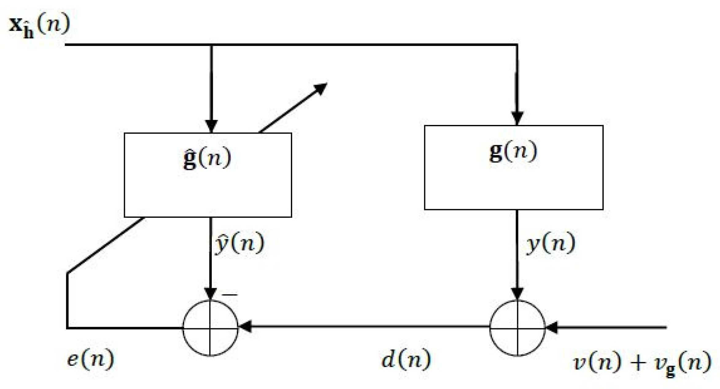
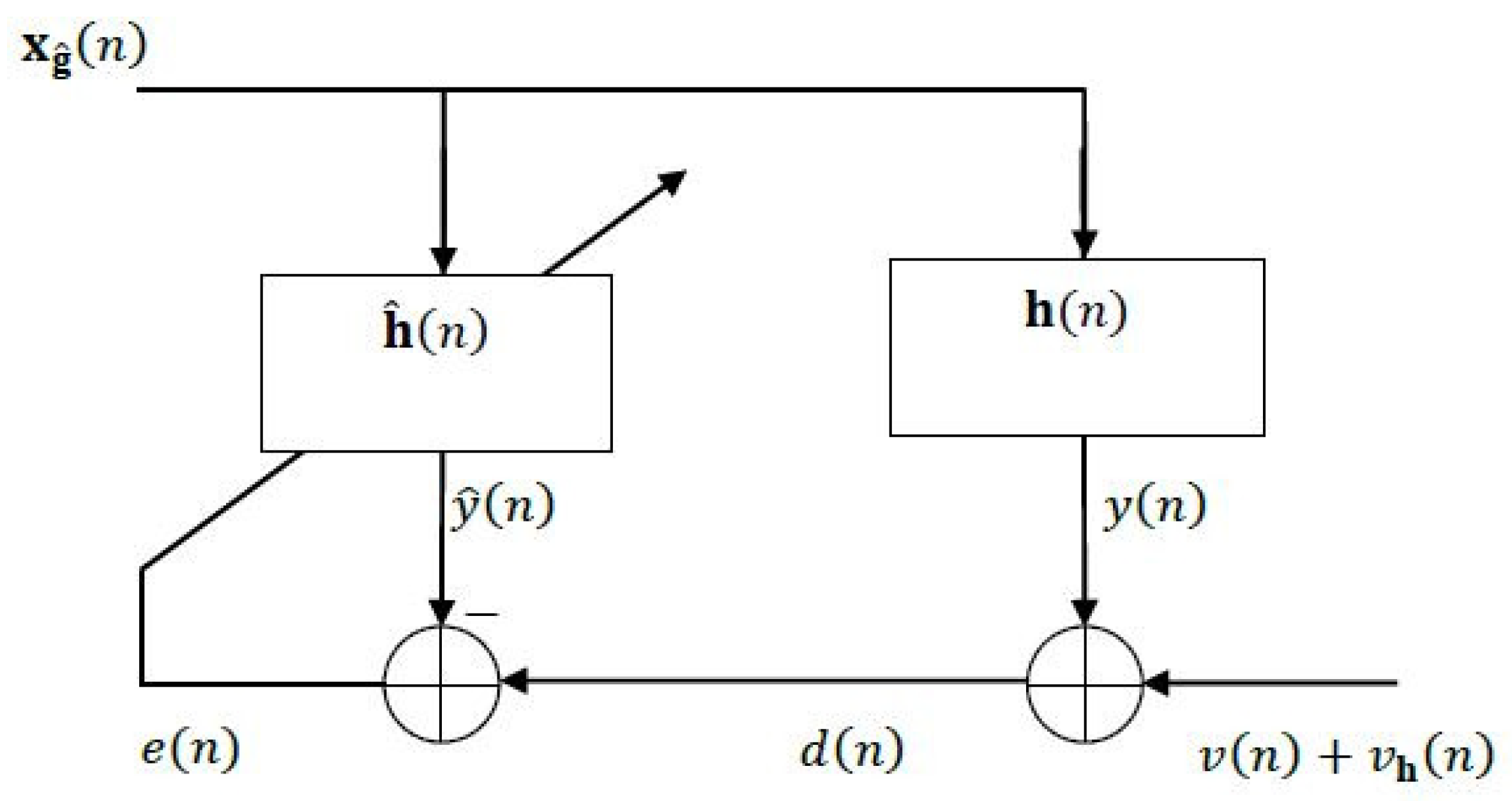
In a similar way, for the second system we have

$$\begin{array}{cc}\hfill d\left(n\right)& ={\mathbf{h}}^T\left(n\right){\mathbf{x}}_{\mathbf{g}}\left(n\right)+{\mathbf{h}}^T\left(n\right){\mathbf{x}}_{\widehat{\mathbf{g}}}\left(n\right)-{\mathbf{h}}^T\left(n\right){\mathbf{x}}_{\widehat{\mathbf{g}}}\left(n\right)+v\left(n\right)\hfill \\ \hfill & ={\mathbf{h}}^T\left(n\right){\mathbf{x}}_{\widehat{\mathbf{g}}}\left(n\right)+v\left(n\right)+v_{\mathbf{h}}\left(n\right),\hfill \end{array}$$

(45)

where

$$\begin{array}{cc}\hfill v_{\mathbf{h}}\left(n\right)& ={\mathbf{h}}^T\left(n\right)\left[{\mathbf{x}}_{\mathbf{g}}\left(n\right)-{\mathbf{x}}_{\widehat{\mathbf{g}}}\left(n\right)\right]\hfill \\ \hfill & ={\mathbf{c}}_{{\mathbf{g}}_{\mathrm{a}}}^T\left(n\right){\mathbf{x}}_{\mathbf{h}}\left(n\right)\hfill \\ \hfill & ={\left[{\mathbf{c}}_{\mathbf{g}}(n-1)+{\overline{\mathbf{w}}}_{\mathbf{g}}\left(n\right)\right]}^T{\mathbf{x}}_{\mathbf{h}}\left(n\right)\hfill \end{array}$$

(46)

can be interpreted as an additional “noise” term, of variance ${\sigma }_{v_{\mathbf{h}}}^2\left(n\right)$, related to the system $\mathbf{h}$. Here, the a posteriori and a priori misalignments corresponding to the system $\mathbf{g}$ were defined in (20) and (22), respectively. In Figure 1 and Figure 2, the equivalent system identification scheme is represented in terms of the two components, $\mathbf{g}\left(n\right)$ and $\mathbf{h}\left(n\right)$, respectively; it can be observed that each system influences the other one through the additional “noise” term.

In the framework of the LMS algorithm for bilinear forms, namely LMS-BF [12], the updates are the following:

$$\begin{array}{cc}\hfill \widehat{\mathbf{g}}\left(n\right)& =\widehat{\mathbf{g}}(n-1)+{\mu }_{\widehat{\mathbf{g}}}{\mathbf{x}}_{\widehat{\mathbf{h}}}\left(n\right)e\left(n\right),\hfill \end{array}$$

(47)

$$\begin{array}{cc}\hfill \widehat{\mathbf{h}}\left(n\right)& =\widehat{\mathbf{h}}(n-1)+{\mu }_{\widehat{\mathbf{h}}}{\mathbf{x}}_{\widehat{\mathbf{g}}}\left(n\right)e\left(n\right),\hfill \end{array}$$

(48)

where ${\mu }_{\widehat{\mathbf{g}}}$ and ${\mu }_{\widehat{\mathbf{h}}}$ are the step-size parameters. In this context, the vectors corresponding to the a posteriori misalignments become

$$\begin{array}{cc}\hfill {\mathbf{c}}_{\mathbf{g}}\left(n\right)& =\mathbf{g}\left(n\right)-\widehat{\mathbf{g}}(n-1)-{\mu }_{\widehat{\mathbf{g}}}{\mathbf{x}}_{\widehat{\mathbf{h}}}\left(n\right)e\left(n\right)\hfill \\ \hfill & ={\mathbf{c}}_{\mathbf{g}}(n-1)+{\overline{\mathbf{w}}}_{\mathbf{g}}\left(n\right)-{\mu }_{\widehat{\mathbf{g}}}{\mathbf{x}}_{\widehat{\mathbf{h}}}\left(n\right)e\left(n\right),\hfill \end{array}$$

(49)

$$\begin{array}{cc}\hfill {\mathbf{c}}_{\mathbf{h}}\left(n\right)& =\mathbf{h}\left(n\right)-\widehat{\mathbf{h}}(n-1)-{\mu }_{\widehat{\mathbf{h}}}{\mathbf{x}}_{\widehat{\mathbf{g}}}\left(n\right)e\left(n\right)\hfill \\ \hfill & ={\mathbf{c}}_{\mathbf{h}}(n-1)+{\overline{\mathbf{w}}}_{\mathbf{h}}\left(n\right)-{\mu }_{\widehat{\mathbf{h}}}{\mathbf{x}}_{\widehat{\mathbf{g}}}\left(n\right)e\left(n\right).\hfill \end{array}$$

(50)

At this point, let us introduce the notation $m_{\mathbf{g}}\left(n\right)=\mathbb{E}\left[\parallel {\mathbf{c}}_{\mathbf{g}}{\left(n\right)\parallel }^2\right]$ and $m_{\mathbf{h}}\left(n\right)=\mathbb{E}\left[\parallel {\mathbf{c}}_{\mathbf{h}}{\left(n\right)\parallel }^2\right]$. Taking the square ${\ell }_2$ norms in both sides of (49) and (50), respectively, we can recursively evaluate

$$\begin{array}{cc}\hfill m_{\mathbf{g}}\left(n\right)& =m_{\mathbf{g}}(n-1)-2{\mu }_{\widehat{\mathbf{g}}}\mathbb{E}\left\{\left[{\mathbf{c}}_{\mathbf{g}}^T(n-1)+{\overline{\mathbf{w}}}_{\mathbf{g}}^T\left(n\right)\right]{\mathbf{x}}_{\widehat{\mathbf{h}}}\left(n\right)e\left(n\right)\right\}+{\mu }_{\widehat{\mathbf{g}}}^2\mathbb{E}\left[{\mathbf{x}}_{\widehat{\mathbf{h}}}^T\left(n\right){\mathbf{x}}_{\widehat{\mathbf{h}}}\left(n\right)e^2\left(n\right)\right]+M{\sigma }_{{\overline{w}}_{\mathbf{g}}}^2\hfill \\ \hfill & =m_{\mathbf{g}}(n-1)-2A_{\mathbf{g}}{\mu }_{\widehat{\mathbf{g}}}+{\mu }_{\widehat{\mathbf{g}}}^2{B}_{\mathbf{g}}+M{\sigma }_{{\overline{w}}_{\mathbf{g}}}^2,\hfill \end{array}$$

(51)

$$\begin{array}{cc}\hfill m_{\mathbf{h}}\left(n\right)& =m_{\mathbf{h}}(n-1)-2{\mu }_{\widehat{\mathbf{h}}}\mathbb{E}\left\{\left[{\mathbf{c}}_{\mathbf{h}}^T(n-1)+{\overline{\mathbf{w}}}_{\mathbf{h}}^T\left(n\right)\right]{\mathbf{x}}_{\widehat{\mathbf{g}}}\left(n\right)e\left(n\right)\right\}+{\mu }_{\widehat{\mathbf{h}}}^2\mathbb{E}\left[{\mathbf{x}}_{\widehat{\mathbf{g}}}^T\left(n\right){\mathbf{x}}_{\widehat{\mathbf{g}}}\left(n\right)e^2\left(n\right)\right]+L{\sigma }_{{\overline{w}}_{\mathbf{h}}}^2\hfill \\ \hfill & =m_{\mathbf{h}}(n-1)-2A_{\mathbf{h}}{\mu }_{\widehat{\mathbf{h}}}+{\mu }_{\widehat{\mathbf{h}}}^2{B}_{\mathbf{h}}+L{\sigma }_{{\overline{w}}_{\mathbf{h}}}^2,\hfill \end{array}$$

(52)

where

$$\begin{array}{cc}\hfill A_{\mathbf{g}}& =\mathbb{E}\left\{\left[{\mathbf{c}}_{\mathbf{g}}^T(n-1)+{\overline{\mathbf{w}}}_{\mathbf{g}}^T\left(n\right)\right]{\mathbf{x}}_{\widehat{\mathbf{h}}}\left(n\right)e\left(n\right)\right\},\hfill \end{array}$$

(53)

$$\begin{array}{cc}\hfill B_{\mathbf{g}}& =\mathbb{E}\left[{\mathbf{x}}_{\widehat{\mathbf{h}}}^T\left(n\right){\mathbf{x}}_{\widehat{\mathbf{h}}}\left(n\right)e^2\left(n\right)\right],\hfill \end{array}$$

(54)

$$\begin{array}{cc}\hfill A_{\mathbf{h}}& =\mathbb{E}\left\{\left[{\mathbf{c}}_{\mathbf{h}}^T(n-1)+{\overline{\mathbf{w}}}_{\mathbf{h}}^T\left(n\right)\right]{\mathbf{x}}_{\widehat{\mathbf{g}}}\left(n\right)e\left(n\right)\right\},\hfill \end{array}$$

(55)

$$\begin{array}{cc}\hfill B_{\mathbf{h}}& =\mathbb{E}\left[{\mathbf{x}}_{\widehat{\mathbf{g}}}^T\left(n\right){\mathbf{x}}_{\widehat{\mathbf{g}}}\left(n\right)e^2\left(n\right)\right].\hfill \end{array}$$

(56)

It is very difficult to further process the expectation terms from (53)–(56) (and, consequently, (51) and (52)) without any supporting assumptions on the character of the input signals. Hence, let us consider that the covariance matrices of the inputs are close to a diagonal one. This is a fairly restrictive assumption on the input signals, which has been widely used to simplify the convergence analysis of many adaptive algorithms [27,28]. Also, let us consider that the input signals are independent and have the same power. In this context, the computations of the expectation terms from (53)–(56) are detailed in Appendix A. Summarizing the results from this appendix, these terms result in

$$\begin{array}{cc}\hfill A_{\mathbf{g}}& =p_{\mathbf{g}}\left(n\right)+{\sigma }_{\mathbf{x}}^2\mathbb{E}\left[{∥\widehat{\mathbf{h}}(n-1)∥}^2\right]\left[m_{\mathbf{g}}(n-1)+M{\sigma }_{{\overline{w}}_{\mathbf{g}}}^2\right],\hfill \end{array}$$

(57)

$$\begin{array}{cc}\hfill A_{\mathbf{h}}& =p_{\mathbf{h}}\left(n\right)+{\sigma }_{\mathbf{x}}^2\mathbb{E}\left[{∥\widehat{\mathbf{g}}(n-1)∥}^2\right]\left[m_{\mathbf{h}}(n-1)+L{\sigma }_{{\overline{w}}_{\mathbf{h}}}^2\right],\hfill \end{array}$$

(58)

$$\begin{array}{cc}\hfill B_{\mathbf{g}}& =M{\sigma }_{\mathbf{x}}^2\mathbb{E}\left[{∥\widehat{\mathbf{h}}(n-1)∥}^2\right]\left\{{\sigma }_v^2+2p_{\mathbf{g}}\left(n\right)+\frac{1}{L}{\sigma }_{v_{\mathbf{g}}}^2\left(n\right)+{\sigma }_{\mathbf{x}}^2\mathbb{E}\left[{∥\widehat{\mathbf{h}}(n-1)∥}^2\right]\left[m_{\mathbf{g}}(n-1)+M{\sigma }_{{\overline{w}}_{\mathbf{g}}}^2\right]\right\},\hfill \end{array}$$

(59)

$$\begin{array}{cc}\hfill B_{\mathbf{h}}& =L{\sigma }_{\mathbf{x}}^2\mathbb{E}\left[{∥\widehat{\mathbf{g}}(n-1)∥}^2\right]\left\{{\sigma }_v^2+2p_{\mathbf{h}}\left(n\right)+\frac{1}{M}{\sigma }_{v_{\mathbf{h}}}^2\left(n\right)+{\sigma }_{\mathbf{x}}^2\mathbb{E}\left[{∥\widehat{\mathbf{g}}(n-1)∥}^2\right]\left[m_{\mathbf{h}}(n-1)+L{\sigma }_{{\overline{w}}_{\mathbf{h}}}^2\right]\right\},\hfill \end{array}$$

(60)

where ${\sigma }_{\mathbf{x}}^2=\mathbb{E}\left[\parallel \tilde{\mathbf{x}}{\left(n\right)\parallel }^2\right]$ and the terms denoted by $p_{\mathbf{g}}\left(n\right)$ and $p_{\mathbf{h}}\left(n\right)$ are evaluated as

$$\begin{array}{cc}\hfill p_{\mathbf{g}}\left(n\right)& =\mathbb{E}\left\{{\mathbf{c}}_{\mathbf{g}}^T(n-1){\mathbf{x}}_{\widehat{\mathbf{h}}}\left(n\right){\tilde{\mathbf{x}}}^T\left(n\right)[\mathbf{g}\otimes {\mathbf{c}}_{\mathbf{h}}(n-1)]\right\}\hfill \\ \hfill & =\mathbb{E}\left\{{\mathbf{c}}_{\mathbf{g}}^T(n-1){\mathbf{x}}_{\widehat{\mathbf{h}}}\left(n\right){\mathbf{c}}_{\mathbf{h}}^T(n-1){\mathbf{x}}_{\mathbf{g}}\left(n\right)\right\},\hfill \end{array}$$

(61)

$$\begin{array}{cc}\hfill p_{\mathbf{h}}\left(n\right)& =\mathbb{E}\left\{{\mathbf{c}}_{\mathbf{h}}^T(n-1){\mathbf{x}}_{\widehat{\mathbf{g}}}\left(n\right){\tilde{\mathbf{x}}}^T\left(n\right)[{\mathbf{c}}_{\mathbf{g}}(n-1)\otimes \mathbf{h}]\right\}\hfill \\ \hfill & =\mathbb{E}\left\{{\mathbf{c}}_{\mathbf{h}}^T(n-1){\mathbf{x}}_{\widehat{\mathbf{g}}}\left(n\right){\mathbf{c}}_{\mathbf{g}}^T(n-1){\mathbf{x}}_{\mathbf{h}}\left(n\right)\right\}.\hfill \end{array}$$

(62)

The expressions of the variances ${\sigma }_{v_{\mathbf{g}}}^2\left(n\right)$ and ${\sigma }_{v_{\mathbf{h}}}^2\left(n\right)$ are also provided in Appendix A. Consequently, using (57)–(60) in (51) and (52), we obtain

$$\begin{array}{cc}\hfill m_{\mathbf{g}}\left(n\right)& =m_{\mathbf{g}}(n-1)\left\{1-2{\mu }_{\widehat{\mathbf{g}}}{\sigma }_{\mathbf{x}}^2\mathbb{E}\left[\parallel \widehat{\mathbf{h}}{(n-1)\parallel }^2\right]+{\mu }_{\widehat{\mathbf{g}}}^2{\sigma }_{\mathbf{x}}^{4}M{\left\{\mathbb{E}\left[\parallel \widehat{\mathbf{h}}{(n-1)\parallel }^2\right]\right\}}^2\right\}-2{\mu }_{\widehat{\mathbf{g}}}{p}_{\mathbf{g}}\left(n\right)\hfill \\ \hfill & +{\mu }_{\widehat{\mathbf{g}}}^{2}M{\sigma }_{\mathbf{x}}^2\mathbb{E}\left[\parallel \widehat{\mathbf{h}}{(n-1)\parallel }^2\right]\left\{{\sigma }_v^2+\frac{1}{L}{\sigma }_{v_{\mathbf{g}}}^2\left(n\right)+M{\sigma }_{{\overline{w}}_{\mathbf{g}}}^2{\sigma }_{\mathbf{x}}^2\mathbb{E}\left[\parallel \widehat{\mathbf{h}}{(n-1)\parallel }^2\right]+2p_{\mathbf{g}}\left(n\right)\right\}\hfill \\ \hfill & +M{\sigma }_{{\overline{w}}_{\mathbf{g}}}^2\left\{1-2{\mu }_{\widehat{\mathbf{g}}}{\sigma }_{\mathbf{x}}^2\mathbb{E}\left[\parallel \widehat{\mathbf{h}}{(n-1)\parallel }^2\right]\right\},\hfill \end{array}$$

(63)

$$\begin{array}{cc}\hfill m_{\mathbf{h}}\left(n\right)& =m_{\mathbf{h}}(n-1)\left\{1-2{\mu }_{\widehat{\mathbf{h}}}{\sigma }_{\mathbf{x}}^2\mathbb{E}\left[\parallel \widehat{\mathbf{g}}{(n-1)\parallel }^2\right]+{\mu }_{\widehat{\mathbf{h}}}^2{\sigma }_{\mathbf{x}}^{4}L{\left\{\mathbb{E}\left[\parallel \widehat{\mathbf{g}}{(n-1)\parallel }^2\right]\right\}}^2\right\}-2{\mu }_{\widehat{\mathbf{h}}}{p}_{\mathbf{h}}\left(n\right)\hfill \\ \hfill & +{\mu }_{\widehat{\mathbf{h}}}^{2}L{\sigma }_{\mathbf{x}}^2\mathbb{E}\left[\parallel \widehat{\mathbf{g}}{(n-1)\parallel }^2\right]\left\{{\sigma }_v^2+\frac{1}{M}{\sigma }_{v_{\mathbf{h}}}^2\left(n\right)+L{\sigma }_{{\overline{w}}_{\mathbf{h}}}^2{\sigma }_{\mathbf{x}}^2\mathbb{E}\left[\parallel \widehat{\mathbf{g}}{(n-1)\parallel }^2\right]+2p_{\mathbf{h}}\left(n\right)\right\}\hfill \\ \hfill & +L{\sigma }_{{\overline{w}}_{\mathbf{h}}}^2\left\{1-2{\mu }_{\widehat{\mathbf{h}}}{\sigma }_{\mathbf{x}}^2\mathbb{E}\left[\parallel \widehat{\mathbf{g}}{(n-1)\parallel }^2\right]\right\}.\hfill \end{array}$$

(64)

In the context of system identification problems, the main goal is to reduce the system misalignment, which basically represents the difference between the true impulse response and the estimated one. Therefore, in our framework, the optimal step-size parameters (denoted in the following by ${\mu }_{\widehat{\mathbf{g}},\mathrm{o}}$ and ${\mu }_{\widehat{\mathbf{h}},\mathrm{o}}$) can be found by minimizing (63) and (64). This is done by canceling the derivatives of (63) and (64) with respect to the step-sizes, which result in:

$$\begin{array}{cc}\hfill \frac{\partial m_{\mathbf{g}}\left(n\right)}{\partial {\mu }_{\widehat{\mathbf{g}}}}& =-2A_{\mathbf{g}}+2B_{\mathbf{g}}{\mu }_{\widehat{\mathbf{g}}}=0\Rightarrow {\mu }_{\widehat{\mathbf{g}},\mathrm{o}}=\frac{A_{\mathbf{g}}}{B_{\mathbf{g}}},\hfill \end{array}$$

(65)

$$\begin{array}{cc}\hfill \frac{\partial m_{\mathbf{h}}\left(n\right)}{\partial {\mu }_{\widehat{\mathbf{h}}}}& =-2A_{\mathbf{h}}+2B_{\mathbf{h}}{\mu }_{\widehat{\mathbf{h}}}=0\Rightarrow {\mu }_{\widehat{\mathbf{h}},\mathrm{o}}=\frac{A_{\mathbf{h}}}{B_{\mathbf{h}}}.\hfill \end{array}$$

(66)

By replacing $A_{\mathbf{g}},B_{\mathbf{g}},A_{\mathbf{h}}$, and $B_{\mathbf{h}}$ with their expressions (see (57)–(60)), the step-size parameters of the proposed optimized LMS algorithm for bilinear forms (namely OLMS-BF) are found. Finally, introducing these parameters in (47) and (48), the updates of the OLMS-BF algorithm become

$$\begin{array}{cc}\hfill \widehat{\mathbf{g}}\left(n\right)& =\widehat{\mathbf{g}}(n-1)+{\mu }_{\widehat{\mathbf{g}},\mathrm{o}}\left(n\right)x_{\widehat{\mathbf{h}}}\left(n\right)e\left(n\right)\hfill \\ \hfill & =\widehat{\mathbf{g}}(n-1)+\frac{x_{\widehat{\mathbf{h}}}\left(n\right)e\left(n\right)}{M{\sigma }_{\mathbf{x}}^2\mathbb{E}\left[\parallel \widehat{\mathbf{h}}{(n-1)\parallel }^2\right]\left\{1+\frac{p_{\mathbf{g}}\left(n\right)+{\sigma }_v^2+\frac{1}{L}{\sigma }_{v_{\mathbf{g}}}^2\left(n\right)}{p_{\mathbf{g}}\left(n\right)+{\sigma }_{\mathbf{x}}^2\mathbb{E}\left[\parallel \widehat{\mathbf{h}}{(n-1)\parallel }^2\right]\left[m_{\mathbf{g}}(n-1)+M{\sigma }_{{\overline{w}}_{\mathbf{g}}}^2\right]}\right\}},\hfill \end{array}$$

(67)

$$\begin{array}{cc}\hfill \widehat{\mathbf{h}}\left(n\right)& =\widehat{\mathbf{h}}(n-1)+{\mu }_{\widehat{\mathbf{h}},\mathrm{o}}\left(n\right)x_{\widehat{\mathbf{g}}}\left(n\right)e\left(n\right)\hfill \\ \hfill & =\widehat{\mathbf{h}}(n-1)+\frac{x_{\widehat{\mathbf{g}}}\left(n\right)e\left(n\right)}{L{\sigma }_{\mathbf{x}}^2\mathbb{E}\left[\parallel \widehat{\mathbf{g}}{(n-1)\parallel }^2\right]\left\{1+\frac{p_{\mathbf{h}}\left(n\right)+{\sigma }_v^2+\frac{1}{M}{\sigma }_{v_{\mathbf{h}}}^2\left(n\right)}{p_{\mathbf{h}}\left(n\right)+{\sigma }_{\mathbf{x}}^2\mathbb{E}\left[\parallel \widehat{\mathbf{g}}{(n-1)\parallel }^2\right]\left[m_{\mathbf{h}}(n-1)+L{\sigma }_{{\overline{w}}_{\mathbf{h}}}^2\right]}\right\}}.\hfill \end{array}$$

(68)

The most problematic terms in (67) and (68) are $p_{\mathbf{g}}\left(n\right)$ and $p_{\mathbf{h}}\left(n\right)$ (from (61) and (62), respectively), which depend on the true impulse responses. However, as shown in the next section, these terms could be omitted in practice.

5. SKF-BF versus OLMS-BF

The SKF-BF and OLMS-BF algorithms were developed following different theoretical patterns. However, there are strong similarities between these two algorithms, as will be explained in this section.

The update equations of the SKF-BF are given by (17) and (18), where the Kalman gain vectors have the expressions in (35) and (36). It can be noticed that the updates of the SKF-BF can be expressed as

$$\begin{array}{cc}\hfill \widehat{\mathbf{g}}\left(n\right)& =\widehat{\mathbf{g}}(n-1)+{\mu }_{\widehat{\mathbf{g}},\mathrm{K}}\left(n\right)x_{\widehat{\mathbf{h}}}\left(n\right)e\left(n\right),\hfill \end{array}$$

(69)

$$\begin{array}{cc}\hfill \widehat{\mathbf{h}}\left(n\right)& =\widehat{\mathbf{h}}(n-1)+{\mu }_{\widehat{\mathbf{h}},\mathrm{K}}\left(n\right)x_{\widehat{\mathbf{g}}}\left(n\right)e\left(n\right),\hfill \end{array}$$

(70)

where the Kalman step-size parameters are

$$\begin{array}{cc}\hfill {\mu }_{\widehat{\mathbf{g}},\mathrm{K}}\left(n\right)& =\frac{1}{{\mathbf{x}}_{\widehat{\mathbf{h}}}^T\left(n\right){\mathbf{x}}_{\widehat{\mathbf{h}}}\left(n\right)\left\{1+\frac{M{\sigma }_v^2}{\left[m_{\mathbf{g}}(n-1)+M{\sigma }_{{\overline{w}}_{\mathbf{g}}}^2\right]{\mathbf{x}}_{\widehat{\mathbf{h}}}^T\left(n\right){\mathbf{x}}_{\widehat{\mathbf{h}}}\left(n\right)}\right\}},\hfill \end{array}$$

(71)

$$\begin{array}{cc}\hfill {\mu }_{\widehat{\mathbf{h}},\mathrm{K}}\left(n\right)& =\frac{1}{{\mathbf{x}}_{\widehat{\mathbf{g}}}^T\left(n\right){\mathbf{x}}_{\widehat{\mathbf{g}}}\left(n\right)\left\{1+\frac{L{\sigma }_v^2}{\left[m_{\mathbf{h}}(n-1)+L{\sigma }_{{\overline{w}}_{\mathbf{h}}}^2\right]{\mathbf{x}}_{\widehat{\mathbf{g}}}^T\left(n\right){\mathbf{x}}_{\widehat{\mathbf{g}}}\left(n\right)}\right\}}.\hfill \end{array}$$

(72)

Comparing these parameters with the optimal step-sizes from (67) and (68) (also taking (A7) and (A8) into account; see Appendix A), we can notice striking resemblances between SKF-BF and OLMS-BF. In fact, these two algorithms are very similar when

$$\begin{array}{cc}\hfill p_{\mathbf{g}}& =p_{\mathbf{h}}=0.\hfill \end{array}$$

(73)

On the other hand, as it was indicated in [12], this could represent a reasonable assumption, since

$$\underset{n\to \infty }{lim}{p}_{\mathbf{g}}\left(n\right)=\underset{n\to \infty }{lim}{p}_{\mathbf{h}}\left(n\right)=0,$$

(74)

suggesting that in the steady-state of the algorithm, the influence of the terms $p_{\mathbf{h}}$ and $p_{\mathbf{g}}$ on the step-size parameters diminishes. As will be supported in simulations, (73) can be fairly imposed within the OLMS-BF algorithm, while still leading to a very good compromise between the performance criteria (e.g., convergence rate versus misadjustment). Under these considerations, the OLMS-BF algorithm is summarized in

Table 3. Optimized LMS algorithm for bilinear forms (OLMS-BF) (practical version, i.e., using (73)).

Initialization:

$\widehat{\mathbf{h}}\left(0\right)={[10\dots 0]}^T,\widehat{\mathbf{g}}\left(0\right)=\frac{1}{M}{[11\dots 1]}^T$

$m_{\mathbf{h}}\left(0\right)={ϵ}_{\mathbf{h}},m_{\mathbf{g}}\left(0\right)={ϵ}_{\mathbf{g}}\left(\mathrm{positive}\mathrm{constants}\right)$

$\mathrm{Parameters}:\mathbb{E}\left[{\parallel \mathbf{h}\left(n\right)\parallel }^2\right],\mathbb{E}\left[{\parallel \mathbf{g}\left(n\right)\parallel }^2\right],{\sigma }_{{\overline{w}}_{\mathbf{h}}}^2,{\sigma }_{{\overline{w}}_{\mathbf{g}}}^2,{\sigma }_v^2\mathrm{known}\mathrm{or}\mathrm{estimated}$

$\mathrm{Algorithm}:$

${\sigma }_{v_{\mathbf{h}}}^2\left(n\right)=M{\sigma }_{\mathbf{x}}^2\mathbb{E}\left[{\parallel \mathbf{h}\left(n\right)\parallel }^2\right]\left[m_{\mathbf{g}}(n-1)+M{\sigma }_{{\overline{w}}_{\mathbf{g}}}^2\right]$

${\sigma }_{v_{\mathbf{g}}}^2\left(n\right)=L{\sigma }_{\mathbf{x}}^2\mathbb{E}\left[{\parallel \mathbf{g}\left(n\right)\parallel }^2\right]\left[m_{\mathbf{h}}(n-1)+L{\sigma }_{{\overline{w}}_{\mathbf{h}}}^2\right]$

$A_{\mathbf{h}}={\sigma }_{\mathbf{x}}^2\mathbb{E}\left[{∥\widehat{\mathbf{g}}(n-1)∥}^2\right]\left[m_{\mathbf{h}}(n-1)+L{\sigma }_{{\overline{w}}_{\mathbf{h}}}^2\right]$

$B_{\mathbf{h}}=L{\sigma }_{\mathbf{x}}^2\mathbb{E}\left[{∥\widehat{\mathbf{g}}(n-1)∥}^2\right]\left\{{\sigma }_v^2+\frac{1}{M}{\sigma }_{v_{\mathbf{h}}}^2\left(n\right)+{\sigma }_{\mathbf{x}}^2\mathbb{E}\left[{∥\widehat{\mathbf{g}}(n-1)∥}^2\right]\left[m_{\mathbf{h}}(n-1)+L{\sigma }_{{\overline{w}}_{\mathbf{h}}}^2\right]\right\}$

$A_{\mathbf{g}}={\sigma }_{\mathbf{x}}^2\mathbb{E}\left[{∥\widehat{\mathbf{h}}(n-1)∥}^2\right]\left[m_{\mathbf{g}}(n-1)+M{\sigma }_{{\overline{w}}_{\mathbf{g}}}^2\right]$

$B_{\mathbf{g}}=M{\sigma }_{\mathbf{x}}^2\mathbb{E}\left[{∥\widehat{\mathbf{h}}(n-1)∥}^2\right]\left\{{\sigma }_v^2+\frac{1}{L}{\sigma }_{v_{\mathbf{g}}}^2\left(n\right)+{\sigma }_{\mathbf{x}}^2\mathbb{E}\left[{∥\widehat{\mathbf{h}}(n-1)∥}^2\right]\left[m_{\mathbf{g}}(n-1)+M{\sigma }_{{\overline{w}}_{\mathbf{g}}}^2\right]\right\}$

${\mu }_{\widehat{\mathbf{h}},\mathrm{o}}=\frac{A_{\mathbf{h}}}{B_{\mathbf{h}}}$

${\mu }_{\widehat{\mathbf{g}},\mathrm{o}}=\frac{A_{\mathbf{g}}}{B_{\mathbf{g}}}$

$e\left(n\right)=d\left(n\right)-{\mathbf{x}}_{\widehat{\mathbf{g}}}^T\left(n\right)\widehat{\mathbf{h}}(n-1)=d\left(n\right)-{\mathbf{x}}_{\widehat{\mathbf{h}}}^T\left(n\right)\widehat{\mathbf{g}}(n-1)$

$\widehat{\mathbf{h}}\left(n\right)=\widehat{\mathbf{h}}(n-1)+{\mu }_{\widehat{\mathbf{h}},\mathrm{o}}{x}_{\widehat{\mathbf{g}}}\left(n\right)e\left(n\right)$

$\widehat{\mathbf{g}}\left(n\right)=\widehat{\mathbf{g}}(n-1)+{\mu }_{\widehat{\mathbf{g}},\mathrm{o}}{x}_{\widehat{\mathbf{h}}}\left(n\right)e\left(n\right)$

$m_{\mathbf{h}}\left(n\right)=m_{\mathbf{h}}(n-1)-2A_{\mathbf{h}}{\mu }_{\widehat{\mathbf{h}},\mathrm{o}}+{\mu }_{\widehat{\mathbf{h}},\mathrm{o}}^2{B}_{\mathbf{h}}+L{\sigma }_{{\overline{w}}_{\mathbf{h}}}^2$

$m_{\mathbf{g}}\left(n\right)=m_{\mathbf{g}}(n-1)-2A_{\mathbf{g}}{\mu }_{\widehat{\mathbf{g}},\mathrm{o}}+{\mu }_{\widehat{\mathbf{g}},\mathrm{o}}^2{B}_{\mathbf{g}}+M{\sigma }_{{\overline{w}}_{\mathbf{g}}}^2$

(in a practical form that facilitates its implementation).

6. Practical Considerations

The previously developed algorithms are designed to identify the individual impulse responses of the bilinear form. The global (spatiotemporal) impulse response can be computed based on the Kronecker product between them. An alternative solution is to use the regular Kalman filter to identify the spatiotemporal impulse response directly, relying on the observation Equation (4) and identifying the state equation:

$$\mathbf{f}\left(n\right)=\mathbf{f}(n-1)+\mathbf{w}\left(n\right),$$

(75)

where $\mathbf{w}\left(n\right)$ is a zero-mean white Gaussian noise signal vector. The covariance matrix of $\mathbf{w}\left(n\right)$ is ${\mathbf{R}}_{\mathbf{w}}\left(n\right)={\sigma }_w^2{\mathbf{I}}_{ML}$, where ${\mathbf{I}}_{ML}$ is the identity matrix of size $ML\times ML$ and the variance ${\sigma }_w^2$ captures the uncertainties in $\mathbf{f}\left(n\right)$.

In this way, following the approach from [26], we can easily derive the regular Kalman filter (KF) and its simplified version (namely SKF), which can identify the global impulse response using a single adaptive filter $\widehat{\mathbf{f}}\left(n\right)$; for further details, please see Sections VI and VII in [26]. However, we need to mention that the solution found using the regular KF and SKF involves an adaptive filter of length $ML$, whereas their counterparts tailored for bilinear forms (i.e., KF-BF and SKF-BF) use two shorter filters of lengths L and M, respectively. As a consequence, besides a lower computational complexity, a much faster converge rate and tracking are expected for the bilinear algorithms with respect to the conventional ones. The same ideas apply for the OLMS-BF algorithm, as compared to its regular counterpart, i.e., the joint-optimized normalized LMS (JO-NLMS) algorithm [29], which could be used to identify the global impulse response $\widehat{\mathbf{f}}\left(n\right)$.

The computational complexity of the previously discussed algorithms is summarized in

Table 4. Computational complexity of the algorithms.

Algorithms	×	+	/
KF-BF [13]	$3(L^2+M^2)+2ML+3L+4M$	$2(L^2+M^2)+2ML+L+2M$	2
KF [26]	$3{\left(ML\right)}^2+4ML$	$2{\left(ML\right)}^2+3ML$	1
SKF-BF (Table 2)	$2ML+2L+3M+6$	$2ML+L+2M+4$	2
SKF [26]	$3ML+6$	$3ML+4$	1
OLMS-BF (Table 3)	$2ML+2L+3M+12$	$2ML+L+2M+8$	2
JO-NLMS [29]	$3ML+6$	$3ML+5$	1

. It can be easily seen that the SKF-BF offer a great reduction in terms of complexity with respect to KF-BF. Also, the SKF-BF and OLMS-BF differ only by a small number of operations, thus confirming the similarity that was highlighted in Section 5. Finally, when $ML\gg M+L$ (which is usually the case in practice), we can notice that the algorithms tailored for bilinear forms (namely KF-BF, SKF-BF, and OLMS-BF) offer lower computational complexities as compared to their regular counterparts (i.e., KF, SKF, and JO-NLMS, respectively).

Next, a few important observations ought to be made regarding the specific parameters that must be set within the algorithms. Here, the noise power ${\sigma }_v^2$ is required in order to compute the Kalman gain vectors (for KF-BF and SKF-BF) or the optimal step-sizes (for OLMS-BF). In practice, we can estimate this parameter in different ways; some simple and efficient methods for this purpose are presented in [30,31]. Although there are different other methods that can be used to estimate the noise power, the analysis of their influence on the performance of the algorithms lies beyond the scope of this paper.

The parameters related to the uncertainties in the unknown systems also need to be set or estimated, i.e., ${\sigma }_{{\overline{w}}_{\mathbf{h}}}^2$ and ${\sigma }_{{\overline{w}}_{\mathbf{g}}}^2$. Choosing small values for these parameters yields a small misalignment, but at the same time a poor tracking. On the other hand, large values (meaning that there are high uncertainties in the unknown systems) lead to a good tracking but also a high misalignment. This means that we always need to have a good compromise between fast tracking and low misalignment. In practice, if we have some a priori information about the systems which we need to identify, we can take it into consideration when setting the values of these parameters. For example, if we assume the spatial impulse response to be time-invariant, we could fix ${\sigma }_{{\overline{w}}_{\mathbf{g}}}^2=0$ and tune only the parameter related to the temporal impulse response. Thus, based on the state equation related to $\mathbf{h}\left(n\right)$, together with the approximation ${∥{\overline{\mathbf{w}}}_{\mathbf{h}}\left(n\right)∥}^2\approx L{\sigma }_{{\overline{w}}_{\mathbf{h}}}^2$ (which is valid when $L\gg 1$), and replacing $\mathbf{h}\left(n\right)$ and $\mathbf{h}(n-1)$ by their estimates, we can evaluate

$${\widehat{\sigma }}_{{\overline{w}}_{\mathbf{h}}}^2\left(n\right)=\frac{1}{L}{∥\widehat{\mathbf{h}}\left(n\right)-\widehat{\mathbf{h}}(n-1)∥}^2.$$

(76)

It can be noticed that the estimation from (76) is designed to achieve a proper compromise between good tracking and low misalignment. When the algorithm starts to converge or when there is an abrupt change of the system, the difference between $\widehat{\mathbf{h}}\left(n\right)$ and $\widehat{\mathbf{h}}(n-1)$ is significant, leading to large values of the parameter ${\widehat{\sigma }}_{{\overline{w}}_{\mathbf{h}}}^2\left(n\right)$, therefore providing fast convergence and tracking. On the contrary, when the algorithm is converging to its steady-state, the difference between $\widehat{\mathbf{h}}\left(n\right)$ and $\widehat{\mathbf{h}}(n-1)$ reduces, thus leading to the parameter ${\widehat{\sigma }}_{{\overline{w}}_{\mathbf{h}}}^2\left(n\right)$ taking small values and, consequently, to a low misalignment.

7. Results

Experiments are performed in the context of system identification, in order to highlight the performance of the Kalman-based algorithms for bilinear forms (referred to as KF-BF and SKF-BF), in comparison with their regular counterparts (KF and SKF, as mentioned in Section 6). Also, we aim to evaluate the features of the OLMS-BF algorithm, as compared to other existing solutions, e.g., the normalized LMS-BF (NLMS-BF) and the JO-NLMS algorithms, which were introduced in [12] and [29], respectively.

In most of the experiments, both the temporal and the spatial impulse responses are randomly generated from a Gaussian distribution, having the lengths equal to $L=64$ and $M=8$, respectively. This leads to a length of the spatiotemporal impulse response equal to $ML=8\times 64=512$. It is also useful to evaluate the tracking capabilities of the algorithms; to this purpose, a sudden change in the temporal impulse response is applied in the middle of simulations, by generating a new random vector of length $L=64$, also from a Gaussian distribution. Only in the last experiment, the impulse response $\mathbf{h}\left(n\right)$ is an acoustic echo path of length $L=512$, while the coefficients of $\mathbf{g}\left(n\right)$ are computed as $g_m\left(n\right)={0.5}^m$, with $m=1,\dots ,M$ and $M=4$; in this case, the length of the global system is $ML=4\times 512=2048$.

The input signals $x_m\left(n\right),m=1,2,\dots ,M$ are either white Gaussian noises (WGNs) or AR(1) processes (which were obtained after passing a white Gaussian noise through a first-order system with the transfer function $1/\left(1-0.8z^{-1}\right)$). The additive noise $v\left(n\right)$ is white and Gaussian, having the variance ${\sigma }_v^2=0.01$; we assume that this parameter is available in the experiments. In most of simulations, the measure of the performance is the NM (in dB) (see (10)), to evaluate the identification of the global impulse response. In addition, in the second set of experiments (focusing on the OLMS-BF algorithm), we also involve the NPMs (based on (8) and (9)), related to the individual impulse responses.

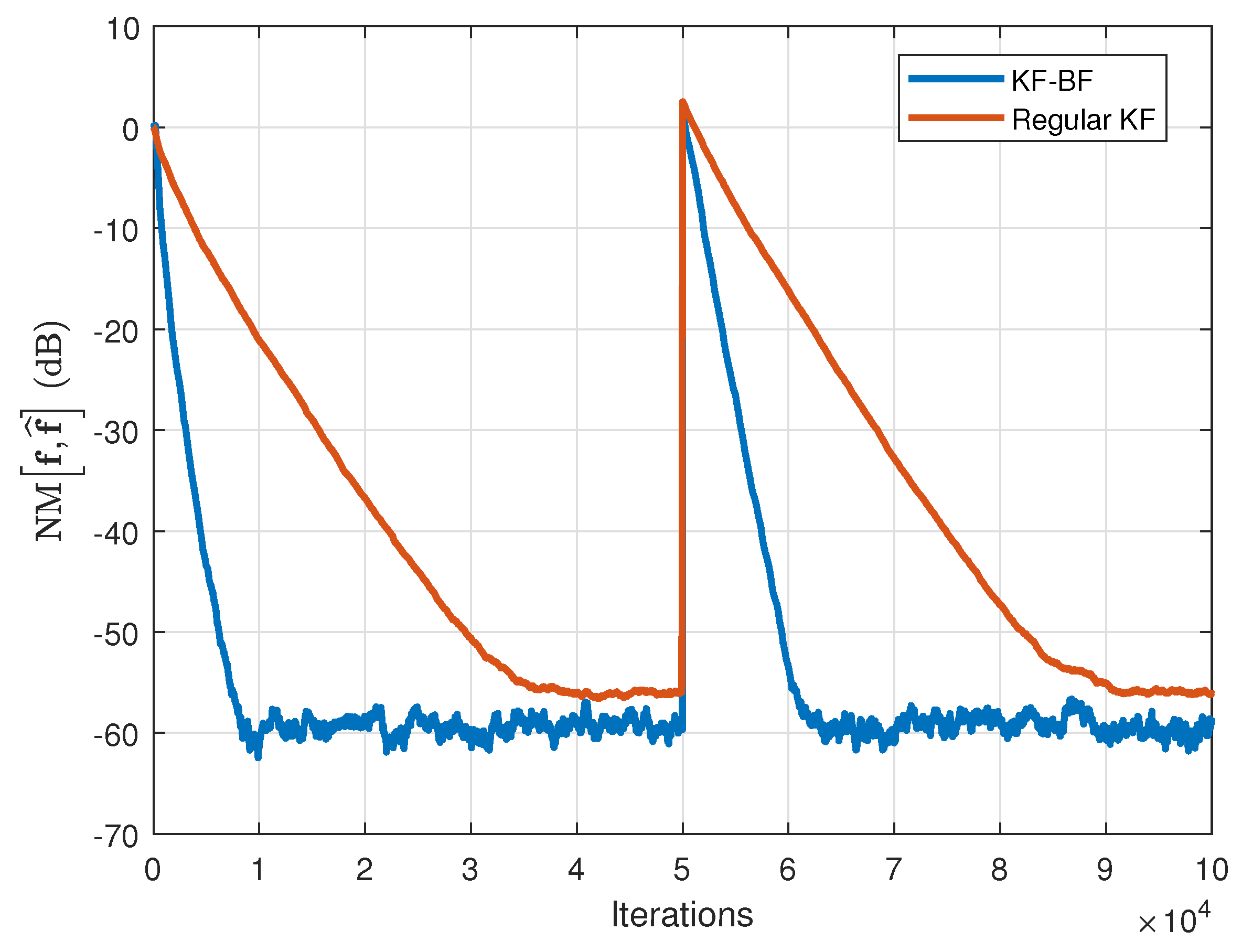
In Figure 3 and Figure 4, the KF-BF is compared to the regular KF for WGN and AR(1) input signals, respectively. The specific parameters of the algorithms are set to ${\sigma }_{{\overline{w}}_{\mathbf{h}}}^2={\sigma }_{{\overline{w}}_{\mathbf{g}}}^2={\sigma }_w^2={10}^{-9}$. It can be noticed from both figures that the KF-BF achieves a faster convergence rate as compared to the regular KF, for both types of input signals, providing also a better tracking capability. The gain is even more apparent in case of AR(1) inputs.

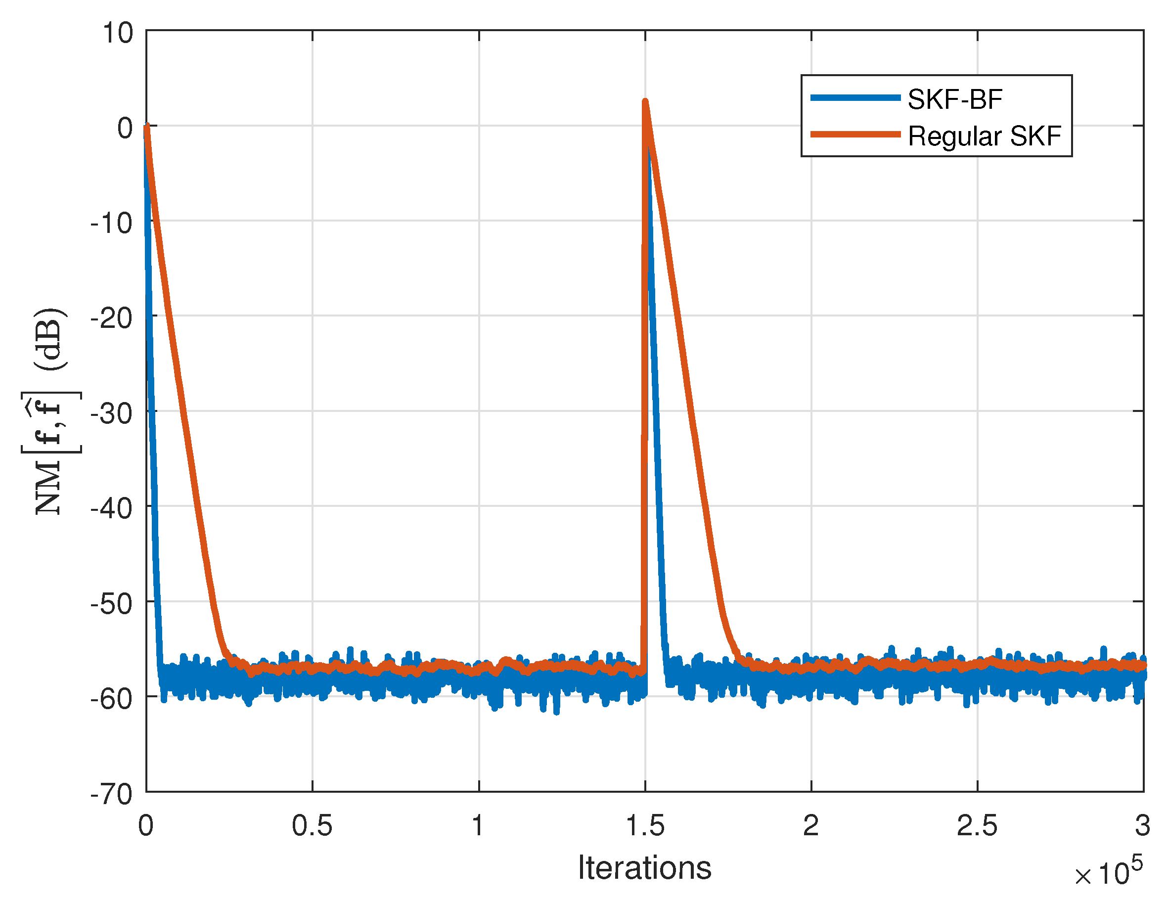
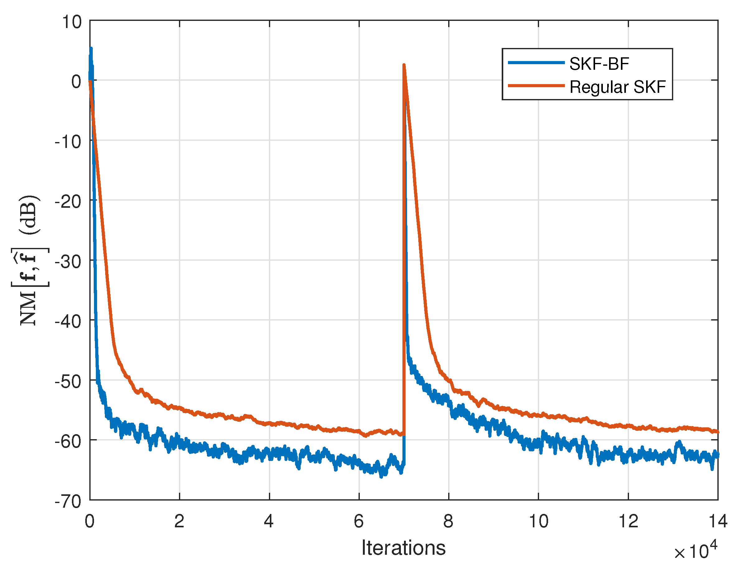
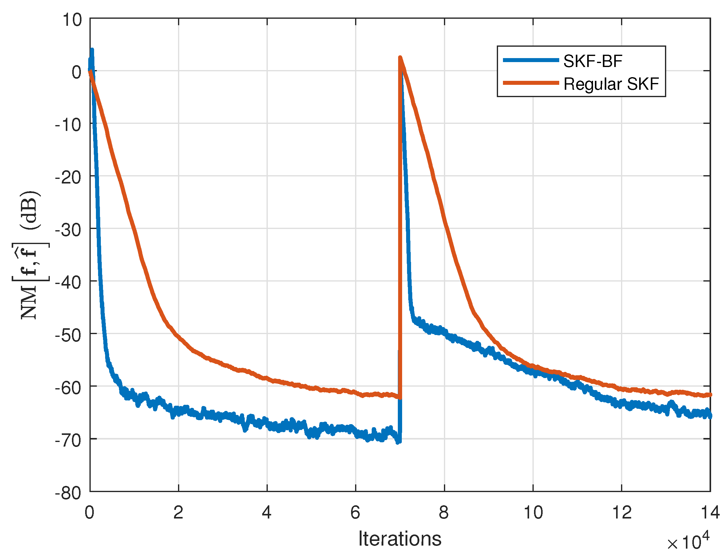
The previous experiment is repeated (for the same two types of inputs) in Figure 5 and Figure 6, this time comparing the SKF-BF with the regular SKF [26]. As it can be observed, the simplified versions (SKF-BF and SKF) yield a slower convergence rate (especially in case of AR(1) inputs) as compared to the full versions (KF-BF and KF, respectively); however, the computational complexities for these simplified versions are much lower. As it was expected, the SKF-BF outperforms the regular SKF in terms of the convergence rate; the improvement is much more visible in the case of AR(1) inputs.

Next, the performance of the SKF-BF is evaluated in Figure 7 and Figure 8, but using the recursive estimation ${\widehat{\sigma }}_{{\overline{w}}_{\mathbf{h}}}^2\left(n\right)$ from (76) (not a constant value, as in the previous experiments). The spatial impulse response is assumed to be time invariant, so that we can set ${\sigma }_{{\overline{w}}_{\mathbf{g}}}^2=0$. The regular SKF is considered for comparison, using a similar way to estimate its specific parameter, i.e., ${\widehat{\sigma }}_w^2\left(n\right)=1/\left(ML\right){∥\widehat{\mathbf{f}}\left(n\right)-\widehat{\mathbf{f}}(n-1)∥}^2$ [26]. Because of the nature of the estimators (as it was explained in Section 6), the algorithms behave like variable step-size adaptive filters, achieving both low misalignment and fast convergence/tracking. Moreover, as we can notice from these two figures, the proposed SKF-BF still outperforms the regular SKF in terms of both performance criteria.

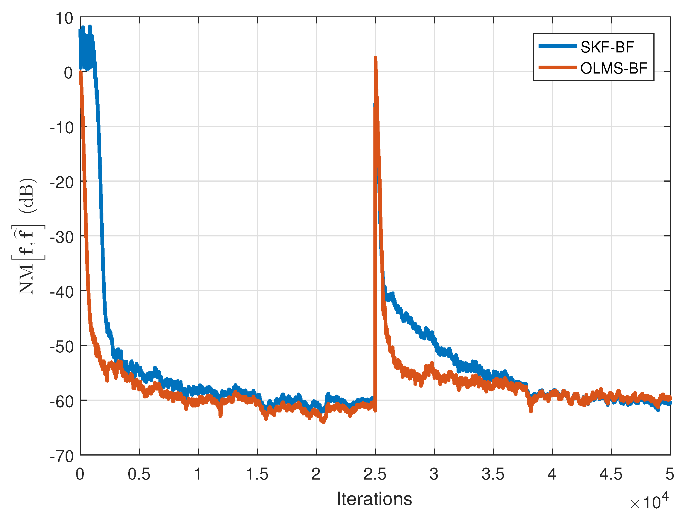
As outlined in Section 5, there are strong similarities between the SKF-BF and OLMS-BF algorithms. In Figure 9 and Figure 10, we compare the performances of these algorithms using two types of input signals, i.e., WGNs and AR(1) processes, respectively. Both algorithms use the recursive estimate ${\widehat{\sigma }}_{{\overline{w}}_{\mathbf{h}}}^2\left(n\right)$ (from (76)) and ${\sigma }_{{\overline{w}}_{\mathbf{g}}}^2=0$. As we can notice, the SKF-BF and OLMS-BF algorithms behave quite similar, especially when the input signals are WGNs (Figure 9). When the input signals are AR(1) processes (Figure 10), the SKF-BF outperforms the OLMS-BF in terms of the initial convergence rate; however, it pays with a slower tracking reaction. Nevertheless, the overall performances of these algorithms are very similar, as supported by the comparison provided in Section 5.

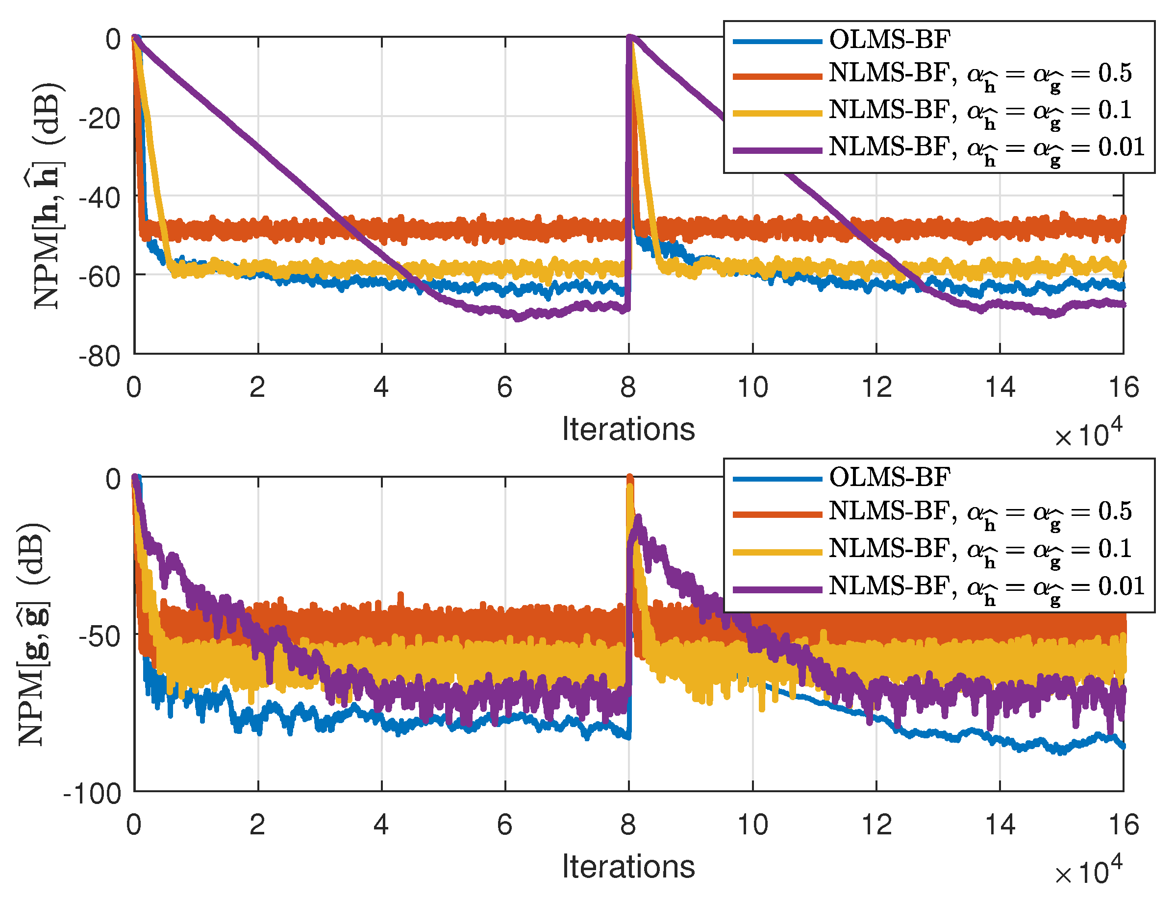
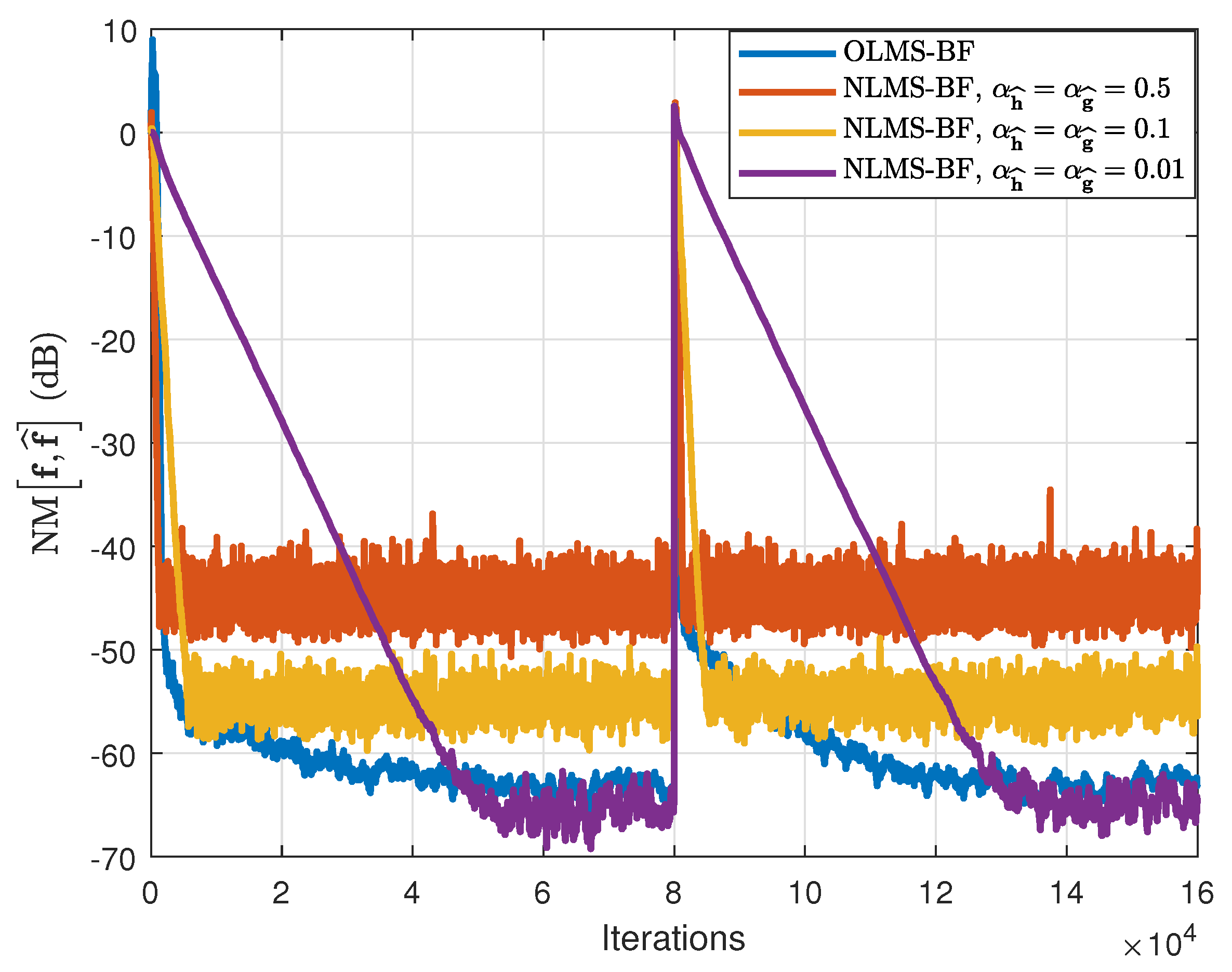
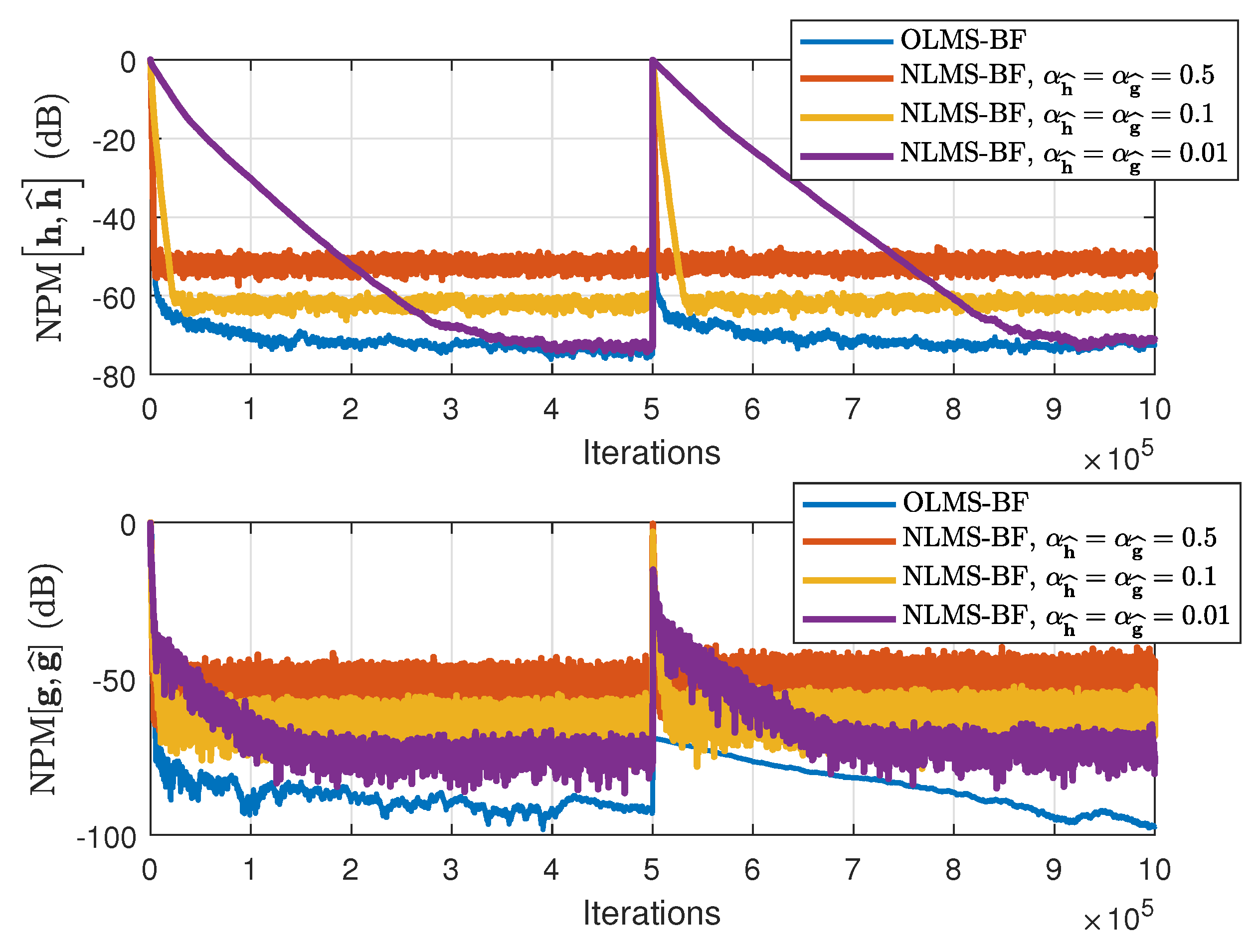
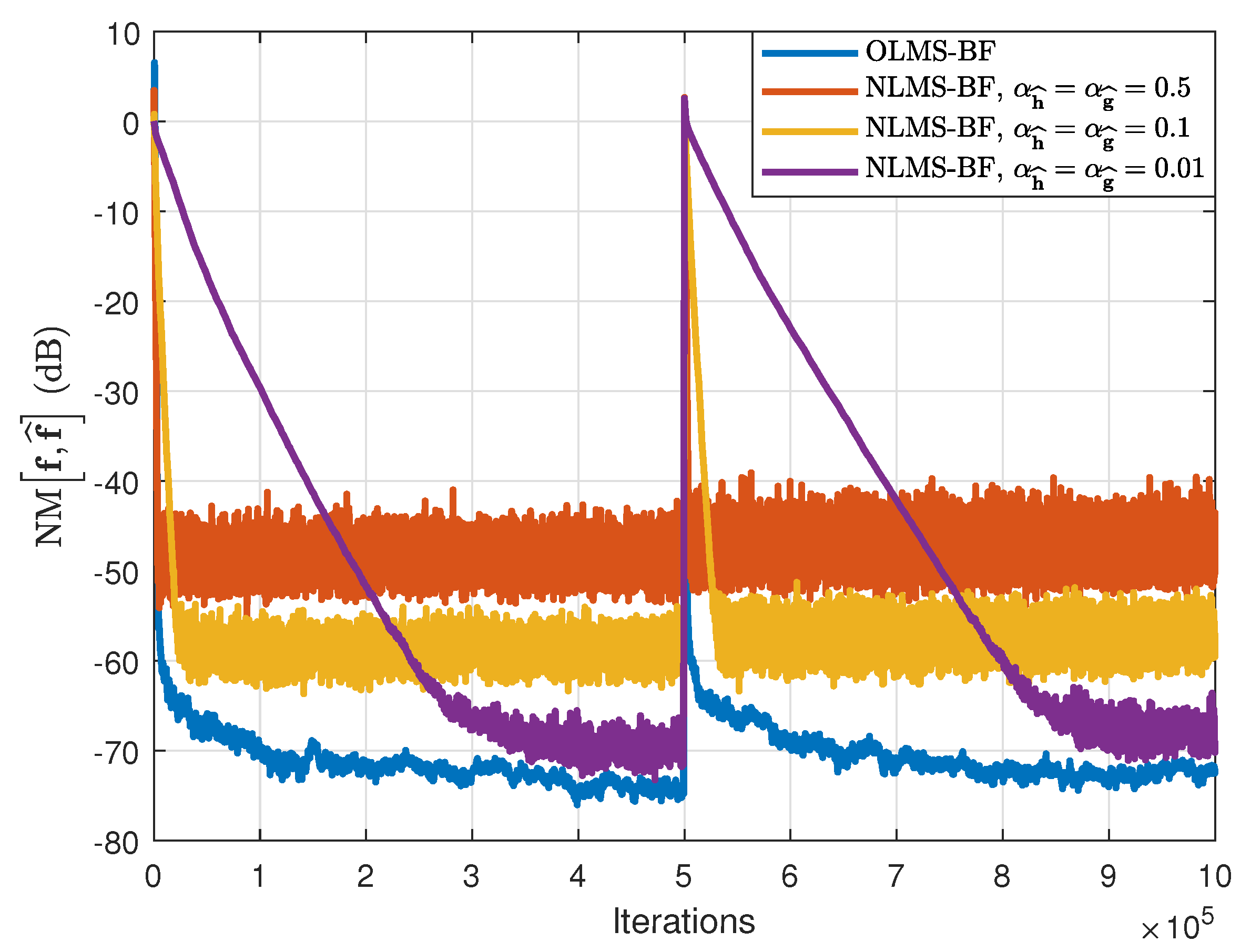
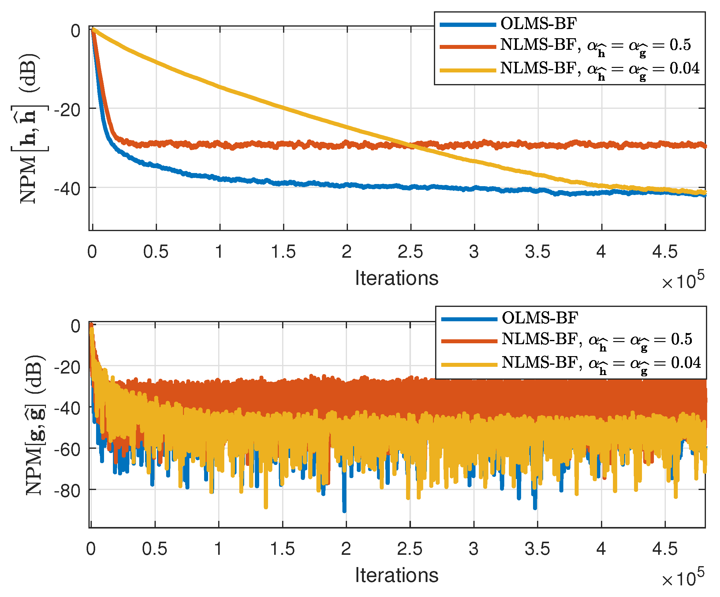
In the second set of experiments, the behavior of the OLMS-BF algorithm is analyzed, as compared to the NLMS-BF algorithm [12]. The NLMS-BF algorithm uses different values of its step-size parameters, ${\alpha }_{\widehat{\mathbf{h}}}$ and ${\alpha }_{\widehat{\mathbf{g}}}$. The performances are now evaluated in terms of both NPMs and NM, using both types of input signals as before (WGNs and AR(1) processes). The results are presented in Figure 11 and Figure 12, using WGNs as inputs, and in Figure 13 and Figure 14, where the input signals are AR(1) processes. It can be noticed that the proposed solution achieves similar convergence rate but a much lower misalignment level than the NLMS-BF algorithm with ${\alpha }_{\widehat{\mathbf{h}}}={\alpha }_{\widehat{\mathbf{g}}}=0.5$ (which provides the fastest convergence rate [12]). On the other hand, if we target a lower misalignment and set the step-sizes of the NLMS-BF to smaller values (i.e., ${\alpha }_{\widehat{\mathbf{h}}}={\alpha }_{\widehat{\mathbf{g}}}=0.1$ and ${\alpha }_{\widehat{\mathbf{h}}}={\alpha }_{\widehat{\mathbf{g}}}=0.01$), the convergence rate also decreases. However, the OLMS-BF algorithm leads to a misalignment level similar to the NLMS-BF algorithm using the smallest step-sizes. In addition, when the input signals are AR(1) processes, the improvement offered by the OLMS-BF algorithm is even more apparent.

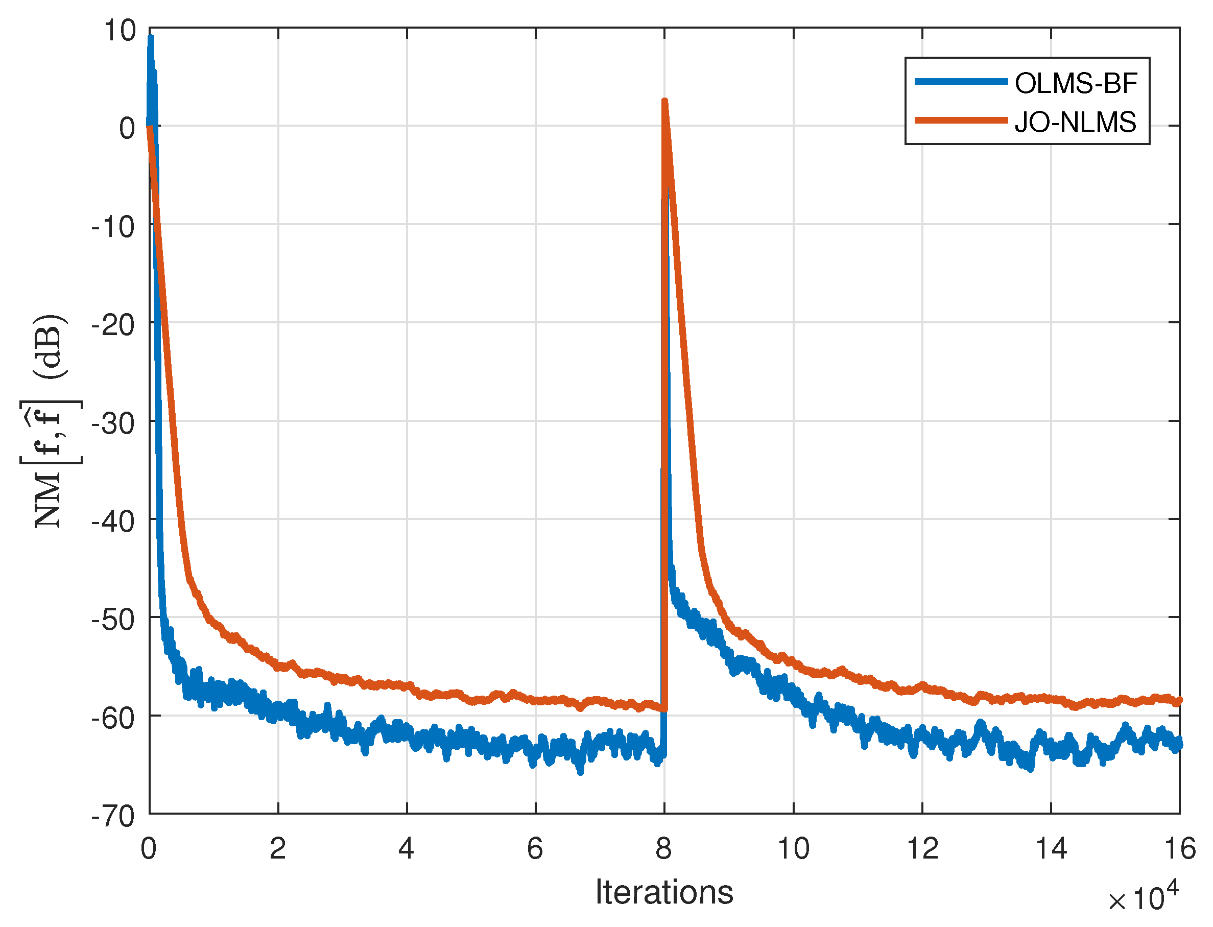
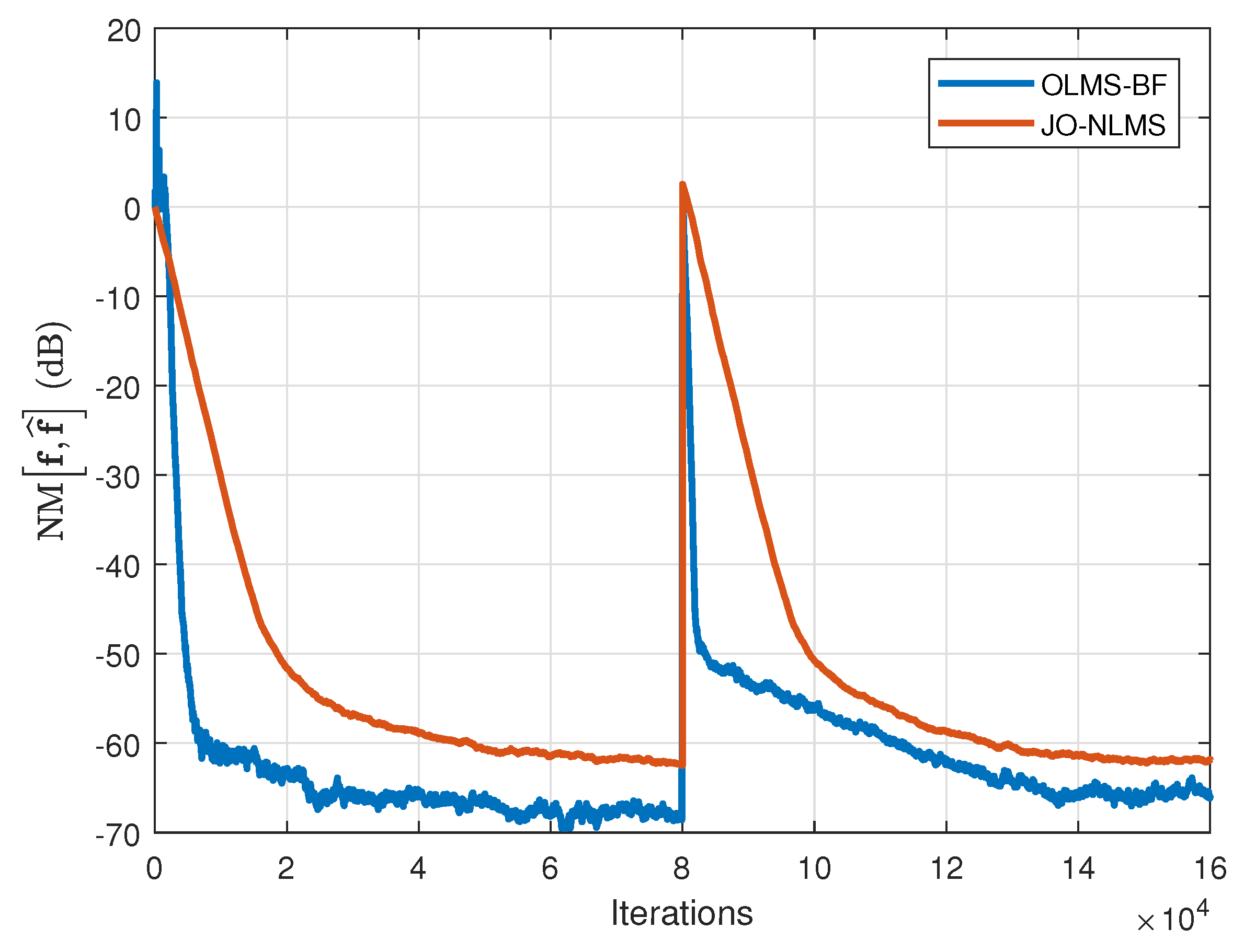
Next, the performance of the OLMS-BF algorithm is evaluated along with the JO-NLMS algorithm [29], which is applied for the identification of the global impulse response of length $ML=512$. The results are presented in Figure 15 and Figure 16, using WGNs and AR(1) input signals, respectively. As specified in Section 6, the JO-NLMS algorithm is the regular counterpart of the OLMS-BF in a classical (one-dimensional) system identification scenario. We can see that the proposed solution (tailored for bilinear forms, i.e., exploiting the two-dimensional decomposition) offers both faster convergence and tracking, as well as a lower misalignment, as compared to the JO-NLMS algorithm. The performance improvement is even more important in case of AR(1) input signals.

Finally, to validate our approach, we assess the performance of the OLMS-BF algorithm when applying it in a context which is closer to a real scenario. The temporal impulse response $\mathbf{h}\left(n\right)$ is a real-world echo path of length $L=512$. The spatial impulse response $\mathbf{g}\left(n\right)$, of length $M=4$, is generated using an exponential decay with the elements $g_m={0.5}^m$, $m=1,\dots ,M$. Both impulse responses are then normalized such that $\parallel \mathbf{h}\left(n\right)\parallel =\parallel \mathbf{g}\left(n\right)\parallel =1$. The input signal is an AR(1) process and we compare the behaviors of the OLMS-BF and NLMS-BF algorithms. The performance is illustrated in Figure 17 and Figure 18. We can notice that the proposed solution slightly outperforms the fastest convergence rate of NLMS-BF, given by ${\alpha }_{\widehat{\mathbf{h}}}={\alpha }_{\widehat{\mathbf{g}}}=0.5$, but at the same time offering a much lower value of the misalignment. If, however, we use the NLMS-BF algorithm with the smaller step-sizes (in order to obtain a better misalignment), the resulting convergence rate is much lower than the one of the OLMS-BF algorithm.

8. Discussion

In this paper, we have focused on the Kalman filter tailored for the identification of bilinear forms (KF-BF), together with its simplified version (SKF-BF). Also, we have developed an optimized version of the LMS algorithm for bilinear forms, namely OLMS-BF. In addition, a comparison between the SKF-BF and OLMS-BF algorithms has been outlined, indicating strong similarities between these two solutions. In our framework, the bilinear term has been defined with respect to the impulse responses of the spatiotemporal model.

The SKF-BF provides a reduced computational complexity as compared to KF-BF; the downside is that it has a slower convergence rate, more visible for correlated inputs. On the other hand, the SKF-BF and OLMS-BF algorithms perform very similarly. Experimental results also indicate that the algorithms tailored for bilinear forms outperform their regular counterparts (in such two-dimensional system identification scenarios), in terms of both convergence rate and tracking, as well as the steady-state misalignment. Adding to that, the reduced computational amount provided by the use of two shorter adaptive filters instead of a single (much longer) one, led us to conclude that the proposed algorithms could represent appealing solutions for the identification of bilinear forms.

References

1. Mohler, R.R.; Kolodziej, W.J. An overview of bilinear system theory and applications. IEEE Trans. Syst. Man Cybern. 1980, 10, 683–688. [Google Scholar]
2. Baik, H.K.; Mathews, V.J. Adaptive lattice bilinear filters. IEEE Trans. Signal Process. 1993, 41, 2033–2046. [Google Scholar] [CrossRef]
3. Han, S.; Kim, J.; Sung, K. Extended generalized total least squares method for the identification of bilinear systems. IEEE Trans. Signal Process. 1996, 44, 1015–1018. [Google Scholar]
4. Tsoulkas, V.; Koukoulas, P.; Kalouptsidis, N. Identification of input-output bilinear systems using cumulants. IEEE Trans. Signal Process. 2001, 51, 2753–2761. [Google Scholar] [CrossRef]
5. Dos Santos, P.L.; Ramos, J.A.; de Carvalho, J.L.M. Identification of bilinear systems with white noise inputs: an iterative deterministic-stochastic subspace approach. IEEE Trans. Control Syst. Technol. 2009, 17, 1145–1153. [Google Scholar] [CrossRef]
6. Forssén, U. Adaptive bilinear digital filters. IEEE Trans. Circuits Syst. II Analog Digital Signal Process. 1993, 40, 729–735. [Google Scholar] [CrossRef]
7. Hu, R.; Hassan, H.M. Echo cancellation in high speed data transmission systems using adaptive layered bilinear filters. IEEE Trans. Commun. 1994, 42, 655–663. [Google Scholar]
8. Zhu, Z.; Leung, H. Adaptive identification of nonlinear systems with application to chaotic communications. IEEE Trans. Circuits Syst. I Fundam. Theory Appl. 2000, 47, 1072–1080. [Google Scholar] [CrossRef]
9. Kuo, S.M.; Wu, H.-T. Nonlinear adaptive bilinear filters for active noise control systems. IEEE Trans. Circuits Syst. I Regul. Pap. 2005, 52, 617–624. [Google Scholar] [CrossRef]
10. Zhao, H.; Zeng, X.; He, Z. Low-complexity nonlinear adaptive filter based on a pipelined bilinear recurrent neural network. IEEE Trans. Neural Netw. 2011, 22, 1494–1507. [Google Scholar] [CrossRef]
11. Benesty, J.; Paleologu, C.; Ciochină, S. On the identification of bilinear forms with the Wiener filter. IEEE Signal Process. Lett. 2017, 24, 653–657. [Google Scholar] [CrossRef]
12. Paleologu, C.; Benesty, J.; Ciochină, S. Adaptive filtering for the identification of bilinear forms. Digital Signal Process. 2018, 75, 153–167. [Google Scholar] [CrossRef]
13. Dogariu, L.; Paleologu, C.; Ciochină, S.; Benesty, J.; Piantanida, P. Identification of bilinear forms with the Kalman filter. In Proceedings of the 2018 IEEE International Conference on Acoustics, Speech and Signal Processing (ICASSP), Calgary, AB, Canada, 15–20 April 2018; pp. 4134–4138. [Google Scholar]
14. Elisei-Iliescu, C.; Stanciu, C.; Paleologu, C.; Benesty, J.; Anghel, C.; Ciochină, S. Efficient recursive least-squares algorithms for the identification of bilinear forms. Digital Signal Process. 2018, 83, 280–296. [Google Scholar] [CrossRef]
15. Gesbert, D.; Duhamel, P. Robust blind joint data/channel estimation based on bilinear optimization. In Proceedings of the 8th Workshop on Statistical Signal and Array Processing, Corfu, Greece, 24–26 June 1996; pp. 168–171. [Google Scholar]
16. Stenger, A.; Kellermann, W.; Rabenstein, R. Adaptation of acoustic echo cancellers incorporating a memoryless nonlinearity. In Proceedings of the IEEE Workshop on Acoustic Echo and Noise Control (IWAENC’99), Pocono Manor, PA, USA, 27–29 September 1999. [Google Scholar]
17. Stenger, A.; Kellermann, W. Adaptation of a memoryless preprocessor for nonlinear acoustic echo cancelling. Signal Process. 2000, 80, 1747–1760. [Google Scholar] [CrossRef] [Green Version]
18. Huang, Y.; Skoglund, J.; Luebs, A. Practically efficient nonlinear acoustic echo cancellers using cascaded block RLS and FLMS adaptive filters. In Proceedings of the 2017 IEEE International Conference on Acoustics, Speech and Signal Processing (ICASSP), New Orleans, LA, USA, 5–9 March 2017; pp. 596–600. [Google Scholar]
19. Kalman, R.E. A new approach to linear filtering and prediction problems. J. Basic Eng. 1960, 82, 35–45. [Google Scholar] [CrossRef]
20. Zarchan, P.; Musoff, H. Fundamentals of Kalman Filtering: A Practical Approach, 4th ed.; American Institute of Aeronautics and Astronautics, Incorporated: Reston, VA, USA, 2015. [Google Scholar]
21. Hsieh, C.-S. Robust two-stage Kalman filters for systems with unknown inputs. IEEE Trans. Autom. Control 2000, 45, 2374–2378. [Google Scholar] [CrossRef]
22. Chen, L.; Mercorelli, P.; Liu, S. A Kalman Estimator for Detecting Repetitive Disturbances. In Proceedings of the 2005, American Control Conference, Portland, OR, USA, 8–10 June 2005; pp. 1631–1636. [Google Scholar]
23. Mercorelli, P. A Motion-Sensorless Control for Intake Valves in Combustion Engines. IEEE Trans. Ind. Electron. 2016, 64, 3402–3412. [Google Scholar] [CrossRef]
24. Morgan, D.R.; Benesty, J.; Sondhi, M.M. On the evaluation of estimated impulse responses. IEEE Signal Process. Lett. 1998, 5, 174–176. [Google Scholar] [CrossRef]
25. Kay, S.M. Fundamentals of Statistical Signal Processing, Volume I: Estimation Theory; Prentice Hall: Englewood Cliffs, NJ, USA, 1993. [Google Scholar]
26. Paleologu, C.; Benesty, J.; Ciochină, S. Study of the general Kalman filter for echo cancellation. IEEE Trans. Audio Speech Lang. Process. 2013, 21, 1539–1549. [Google Scholar] [CrossRef]
27. Haykin, S.; Widrow, B. (Eds.) Least-Mean-Square Adaptive Filters; Wiley: Hoboken, NJ, USA, 2003. [Google Scholar]
28. Sulyman, A.I.; Zerguine, A. Convergence and steady-state analysis of a variable step-size NLMS algorithm. Signal Process. 2003, 83, 1255–1273. [Google Scholar] [CrossRef]
29. Ciochină, S.; Paleologu, C.; Benesty, J. An optimized NLMS algorithm for system identification. Signal Process. 2016, 118, 115–121. [Google Scholar] [CrossRef]
30. Iqbal, M.A.; Grant, S.L. Novel variable step size NLMS algorithm for echo cancellation. In Proceedings of the 2008 IEEE International Conference on Acoustics, Speech and Signal Processing, Las Vegas, NV, USA, 31 March–4 April 2008; pp. 241–244. [Google Scholar]
31. Paleologu, C.; Ciochină, S.; Benesty, J. Double-talk robust VSS-NLMS algorithm for under-modeling acoustic echo cancellation. In Proceedings of the 2008 IEEE International Conference on Acoustics, Speech and Signal Processing, Las Vegas, NV, USA, 31 March–4 April 2008; pp. 245–248. [Google Scholar]
Figure 1. Equivalent system identification scheme when considering the system g ( n ) and the input x h ^ ( n ) .
Algorithms 11 00211 g001
Figure 2. Equivalent system identification scheme when considering the system h ( n ) and the input x g ^ ( n ) .
Algorithms 11 00211 g002
Figure 3. Normalized misalignment of the KF-BF and regular KF using WGNs as input signals. The length of the global impulse response is M L = 512 . The specific parameters are set to σ w ¯ h 2 = σ w ¯ g 2 = σ w 2 = 10 9 .
Algorithms 11 00211 g003
Figure 4. Normalized misalignment of the KF-BF and regular KF using AR(1) processes as input signals. The length of the global impulse response is M L = 512 . The specific parameters are set to σ w ¯ h 2 = σ w ¯ g 2 = σ w 2 = 10 9 .
Algorithms 11 00211 g004
Figure 5. Normalized misalignment of the SKF-BF and regular SKF using WGNs as input signals. The length of the global impulse response is M L = 512 . The specific parameters are set to σ w ¯ h 2 = σ w ¯ g 2 = σ w 2 = 10 9 .
Algorithms 11 00211 g005
Figure 6. Normalized misalignment of the SKF-BF and regular SKF using AR(1) processes as input signals. The length of the global impulse response is M L = 512 . The specific parameters are set to σ w ¯ h 2 = σ w ¯ g 2 = σ w 2 = 10 9 .
Algorithms 11 00211 g006
Figure 7. Normalized misalignment of the SKF-BF and regular SKF (for WGNs input signals), using the recursive estimates σ ^ w ¯ h 2 ( n ) and σ ^ w 2 ( n ) , respectively; the SKF-BF uses σ w ¯ g 2 = 0 . The length of the global impulse responses is M L = 512 .
Algorithms 11 00211 g007
Figure 8. Normalized misalignment of the SKF-BF and regular SKF (for AR(1) input signals), using the recursive estimates σ ^ w ¯ h 2 ( n ) and σ ^ w 2 ( n ) , respectively; the SKF-BF uses σ w ¯ g 2 = 0 . The length of the global impulse responses is M L = 512 .
Algorithms 11 00211 g008
Figure 9. Normalized misalignment of the SKF-BF and OLMS-BF algorithms using WGNs as input signals. Both algorithms use the recursive estimate σ ^ w ¯ h 2 ( n ) and σ w ¯ g 2 = 0 . The length of the global impulse responses is M L = 512 .
Algorithms 11 00211 g009
Figure 10. Normalized misalignment of the SKF-BF and OLMS-BF algorithms using AR(1) processes as input signals. Both algorithms use the recursive estimate σ ^ w ¯ h 2 ( n ) and σ w ¯ g 2 = 0 . The length of the global impulse responses is M L = 512 .
Algorithms 11 00211 g010
Figure 11. Normalized projection misalignment of the OLMS-BF and NLMS-BF (using different step-size parameters): (Top) identification of the temporal impulse response h ( n ) , (Bottom) identification of the spatial impulse response g ( n ) . The input signals are WGNs, L = 64 , and M = 8 .
Algorithms 11 00211 g011
Figure 12. Normalized misalignment of the OLMS-BF and NLMS-BF (using different step-size parameters). The input signals are WGNs and M L = 512 .
Algorithms 11 00211 g012
Figure 13. Normalized projection misalignment of the OLMS-BF and NLMS-BF (using different step-size parameters): (Top) identification of the temporal impulse response h ( n ) , (Bottom) identification of the spatial impulse response g ( n ) . The input signals are AR(1) processes, L = 64 , and M = 8 .
Algorithms 11 00211 g013
Figure 14. Normalized misalignment of the OLMS-BF and NLMS-BF (using different step-size parameters). The input signals are AR(1) processes and M L = 512 .
Algorithms 11 00211 g014
Figure 15. Normalized misalignment of the OLMS-BF and regular JO-NLMS algorithms. The input signals are WGNs and M L = 512 .
Algorithms 11 00211 g015
Figure 16. Normalized misalignment of the OLMS-BF and regular JO-NLMS algorithms. The input signals are AR(1) processes and M L = 512 .
Algorithms 11 00211 g016
Figure 17. Normalized projection misalignment of the OLMS-BF and NLMS-BF (using different step-size parameters): (Top) identification of the temporal impulse response h ( n ) , (Bottom) identification of the spatial impulse response g ( n ) . The input signals are AR(1) processes, L = 512 , and M = 4 .
Algorithms 11 00211 g017
Figure 18. Normalized misalignment of the OLMS-BF and NLMS-BF (using different step-size parameters). The input signals are AR(1) processes and M L = 2048 .
Algorithms 11 00211 g018