Article

Research on Misalignment Fault Isolation of Wind Turbines Based on the Mixed-Domain Features

School of Mechanical, Electronic and Control Engineering, Beijing Jiaotong University, Beijing 100044, China
*
Author to whom correspondence should be addressed.
Algorithms 2017, 10(2), 67; https://doi.org/10.3390/a10020067
Submission received: 2 May 2017 / Revised: 7 June 2017 / Accepted: 8 June 2017 / Published: 10 June 2017

Abstract

:
The misalignment of the drive system of the DFIG (Doubly Fed Induction Generator) wind turbine is one of the important factors that cause damage to the gears, bearings of the high-speed gearbox and the generator bearings. How to use the limited information to accurately determine the type of failure has become a difficult study for the scholars. In this paper, the time-domain indexes and frequency-domain indexes are extracted by using the vibration signals of various misaligned simulation conditions of the wind turbine drive system, and the time-frequency domain features—energy entropy are also extracted by the IEMD (Improved Empirical Mode Decomposition). A mixed-domain feature set is constructed by them. Then, SVM (Support Vector Machine) is used as the classifier, the mixed-domain features are used as the inputs of SVM, and PSO (Particle Swarm Optimization) is used to optimize the parameters of SVM. The fault types of misalignment are classified successfully. Compared with other methods, the accuracy of the given fault isolation model is improved.

1. Introduction

With the rapid development of wind power, a lot of wind turbines have faults in the operation because most of them are installed in remote areas, and their loads are unstable. The operation and maintenance cost of up to 25–30% seriously restrict the development of wind power industry [1,2]. Therefore, how to reduce the risk of wind turbine operation and decrease the cost of wind power generation has become a research topic for many scholars. The fault isolation of wind turbine is the bottleneck to solve the above problems; undoubtedly, it is the key to ensuring long-term stable operation of the wind turbine, and it is the necessary means to realize the condition-based maintenance of the wind turbines [3].
Variable speed constant frequency doubly fed wind turbine is the main type in wind farms [4], and its simplified model is shown in Figure 1. The fault rate of gearbox and generator is relatively high [5]. There are many reasons for the faults of gearbox and generator, and the misalignment between them is one of the most important [6]. This is mostly because:
  • The precise alignment in the wind turbine is very difficult;
  • The wind speed fluctuation can cause the start-stop of wind turbine frequently, and, as time goes on, it will cause the shift of generator or the deformation of some parts, resulting in the misalignment of generator and gearbox.
When the misalignment occurs, it is easy to cause damage to gearbox gears, bearings and generator bearings and so on. Therefore, the study and fault isolation of the transmission system in the wind turbine is the key to ensuring its long stable operation.
The misalignment belongs to a latent fault. When the fault is accumulated to a certain extent, the equipment is damaged seriously, leading to the outage of the wind turbine, affecting the power generation seriously, resulting in huge economic losses. For many years, how to isolate the latent fault accurately has been a difficult problem. This is mainly due to the fault feature of latent faults not being obvious, and researchers lack the awareness of the developing rules for latent fault. In order to identify and isolate the existence of the misalignment fault accurately and to overcome the difficulty of obtaining a large number of misalignment fault samples in reality, in this paper, Solidworks and Adams models are established according to the 1.5 MW wind turbine. The simulation of the transmission system is carried out in Adams under the normal operation, the parallel misalignment, the angle misalignment and the comprehensive misalignment. The vibration signal (angular acceleration) of a high speed shaft is extracted as the information (the established model and its effectiveness are shown in [7]).
The methods of extracting fault features from vibration signals are mainly based on time-domain analysis, frequency-domain analysis and time-frequency domain analysis:
  • The time-domain analysis is one of the most simple and direct analysis methods, and it is effective in isolating the fault in a certain extent. Except for the poor anti-interference of serious faults, the numerical values in time-domain are close to that in normal state, so it is easy to make misjudgments only using time-domain analysis.
  • The frequency-domain analysis of signal is the most commonly used method of mechanical equipment fault analysis. It can be used to get more intuitive fault information than by the time-domain analysis. However, the theoretical basis of frequency-domain analysis is the method of Fourier analysis, so it has sidedness, and cannot extract the features of vibration signal comprehensively.
  • The vibration signal is expressed in the time-domain and frequency-domain at the same time for the time-frequency domain analysis, and it has very prominent advantages. The main methods of feature extraction based on time-frequency analysis are as follows: short time Fourier Transform, Wigner-Ville Distribution, Wavelet Transform, Blind Source Separation, Empirical Mode Decomposition (EMD) and so on.
Due to the complexity of the fault mechanism of the wind turbine transmission system, the state information is different with different feature indexes, the sensitivity and regularity of the running state, as well as the clustering and separability in the model space not being the same. Single features or single domain features are difficult to fully reflect the different conditions of wind turbines with different degrees and types of faults. Therefore, it is necessary to construct a mixed feature library with time-domain, frequency-domain and time-frequency domain, which becomes one of the development trends of fault feature extraction.
Many scholars have applied one or two of the above domains to extract the fault isolation feature based on vibration signal. For example, Ref. [8] extracted root mean square (RMS), peak value and kurtosis coefficient of the vibration signal, and combined with the time-domain waveform to judge whether there was fault in equipment. In Ref. [9], the kurtosis and peak value of the vibration signal were selected as the time-domain indexes, and then the wavelet packet algorithm was used to extract the frequency band energy and the 2-norm as the time-frequency domain indexes, the PCA (Principal Component Analysis) was used to confirm the principal component, and the crack fault of the wind turbine gearbox was diagnosed effectively. The EMD method was used to judge the working states and fault types of the gear by calculating EMD energy entropy of different vibration signals as the input features of Support Vector Machine in [10], but only the time-frequency domain feature was considered. Ref. [11] used a testing system for a wind turbine vibration test to collect vibration signal, and the time-domain and frequency-domain analysis were carried out to get the fault features of the rotor misalignment through the analysis of wind turbine generator, but the time-frequency analysis was not considered. In Ref. [12], the wavelet analysis was used to denoise the vibration signals of the wind turbine gearbox under normal, wear fault and broken tooth fault. Five feature parameters were extracted into the LVQ (Learning Vector Quantification) neural network, and the results showed that the method can identify the fault quickly and accurately. In Ref. [13], the time-domain of the peak, RMS and kurtosis of the vibration signal were extracted as the time-domain features of the fault gearbox. Combining observation and analysis of the normal signal and fault signal frequency-domain feature, the possible location of the failure was determined. In Ref. [14], the vibration signals of three typical states of normal conditions, tooth wear and tooth breakage of the gearbox in the wind turbine are analyzed, and the margin index, kurtosis index, peak index, pulse index, power spectrum entropy in the frequency-domain were extracted, the time-domain and frequency-domain features were the inputs in the fault isolation. In Refs. [15] and [16], the mixed-domain feature set is constructed to completely characterize the property of each fault by combining Empirical Mode Decomposition (EMD) with the Autoregression (AR) model coefficients.
A large amount of literature shows that there are few reports on the method of combining the time-domain, frequency-domain and time-frequency domain features together to construct a mixed-domain feature library when researching the fault of the wind turbine transmission system. In order to extract the feature parameters which reflect the vibration signal as much as possible, and to make the fault isolation more reliable and accurate, in this paper, firstly, the time-domain, frequency-domain and time-frequency domain of the wind turbine vibration signal are combined to construct the mixed-domain feature library to obtain more comprehensive and accurate fault isolation information. The information entropy of the intrinsic mode function (IMF) component decomposed by EMD is used as the time-frequency feature. Then, the support vector machine that is suitable for small samples is used as the isolation tool, and the PSO algorithm is used to optimize the relevant parameters of the support vector machine to obtain better classification performance with high diagnostic accuracy. The results show that the proposed method can identify the types of misalignment effectively compared with other methods.

2. Establishment of Mixed-Domain Feature Library

2.1. Feature Extraction of Vibration Signal in the Time-Domain

The vibration signal of the transmission system (assuming that the signal is a discrete time series x 0 , x 1 , x 2 , ... , x N 1 with finite length) contains the running status information, so a representative time-domain index can be selected as the fault feature parameter to help determine whether the drive system has a fault and what type of misalignment has occurred. The time-domain features of the signal include the dimensional and the dimensionless time-domain index [17].

2.1.1. Dimensional Index

In this paper, the dimensional time-domain indexes selected include the variance, the square root amplitude, the RMS, the standard deviation (SD) and the kurtosis. Their formulas are as follows:
Variance:
σ 2 = 1 N i = 0 N 1 ( x i x ¯ ) 2 = x a x ¯ 2 ,
where x ¯ is the mean of the signal.
Square root amplitude:
x r = ( 1 N i = 0 N 1 | x i | 1 / 2 ) 2 ,
RMS:
x r m s = ( 1 N i = 0 N = 1 x i 2 ) 1 / 2 ,
SD:
x s t d = ( 1 N i = 1 N ( x i x ¯ ) 2 ) 1 / 2 ,
Kurtosis:
β = 1 N i = 1 N x i 4 .

2.1.2. Dimensionless Index

The dimensionless index is not so sensitive to the change of amplitude and frequency of the signal, that is, it is not directly related to the working parameters of the wind turbine. The kurtosis index, the waveform index, the peak index, the pulse index and the margin index are commonly used as dimensionless indexes [18].
The impact component will be produced when there is fault in the transmission system of wind turbine, and the kurtosis index can reflect the degree of steepness, and the expression is:
x q = 1 N i = 0 N 1 x i 4 / x a 2 .
The waveform index reflects the shape of the time-domain waveform, which is sensitive to the waveform change caused by the fault, and the expression is:
K = x r m s x .
The peak index reflects the distribution of large data components in the vibration signal, which is the deviation degree of the vibration amplitude distribution relative to the normal Gaussian distribution, and the expression is:
C = x p x r m s .
The pulse index represents the magnitude of the impact component in the signal, which is sensitive at the beginning of the fault, and the expression is:
I = x p x .
The margin index is sensitive to the impact signal, and the expression is:
L = x p x r .

2.2. Feature Extraction of Vibration Signal in the Frequency-Domain

For a complex vibration signal, the information extracted in the time-domain is limited. Therefore, the time-domain signal is often transformed into a frequency-domain signal by a mathematical method to reveal the frequency component of the signal, so as to extract more information from the signal. The mathematical basis for the transition from time-domain to frequency-domain is Fourier Transform. The process of Fourier Transform is called spectrum analysis. The commonly used spectral analysis includes amplitude spectrum analysis, phase spectrum analysis, logarithmic spectrum analysis and power spectrum analysis. Power spectrum is a commonly used method for frequency-domain feature extraction. It can be used to describe the change of signal frequency-domain features by describing the change of power centroid and the dispersion degree of power distribution [19].
For a discrete time series ( x 0 , x 1 , x 2 , ... , x N 1 ) with finite length, assuming the sampling frequency is f s , three commonly used frequency-domain parameters are as follows [20]:
Centroid frequency (FC):
F C = 1 2 π f s · 0 π ω S ( ω ) d ω 0 π S ( ω ) d ω ,
Mean square Frequency (MSF):
M S F = 1 4 π 2 f s 2 · 0 π ω 2 S ( ω ) d ω 0 π S ( ω ) d ω ,
Variance frequency (VF):
V F = 1 4 π 2 f s 2 · 0 π ( ω 2 π f s F C ) S ( ω ) d ω 0 π S ( ω ) d ω = M S F F C 2 ,
where S ( ω ) is power spectrum of the discrete signal, S ( ω ) = X ( ω ) · X ( ω ) ¯ , X ( ω ) = i = 0 N 1 x ( i ) e j π ω ; and ω is the angular frequency.

2.3. Feature Extraction of Vibration Signal in the Time-Frequency Domain

In this paper, EMD is improved by the method of mirror extension, and the energy entropy of the vibration signal is extracted by the improved EMD (IEMD).
Assuming [21]:
E i = | c i ( t ) | 2 d t = k = 1 n | x i k 2 | ,
E = i = 1 n E i ,
p i = E i E ,
where i = 1 , 2 , 3 , ... , n ; x i k is the amplitude of each discrete point.
The expression of IEMD energy entropy is
P i = i = 1 n p i lg p i .
According to Ref. [7], the energy entropy of the first eight IMF components of IEMD decomposition is the time-frequency domain indexes.
Collecting the vibration signal of the high-speed shaft at normal and three misalignment conditions with the speeds of 81.3°/s, 104.4°/s, 110.7°/s and 117.0°/s, respectively, one gets 114 samples at each speed with each case, so the total number of samples is 4 × 4 × 114. The features of time-domain, frequency-domain and time-frequency domain of the samples are extracted to construct the mixed-domain fault feature library, which are shown in Table 1.
Table 2, Table 3 and Table 4 are partial data of the extracted time-domain, frequency-domain and time-frequency domain indexes. Type 0, 1, 2, 3 represent normal state, parallel misalignment, angle misalignment and comprehensive misalignment, respectively.

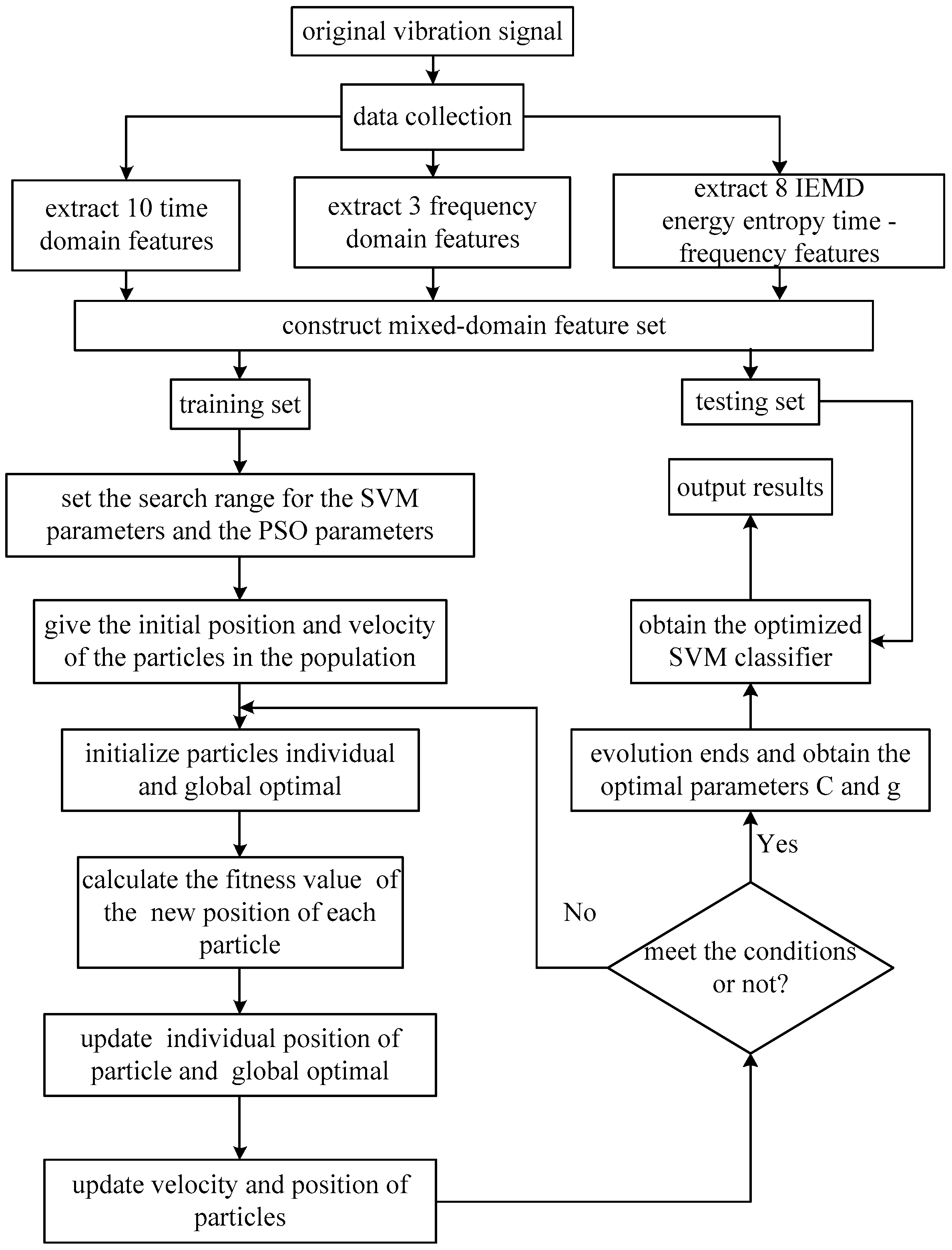
3. Fault Isolation of Transmission System Based on PSO-SVM

After establishing the mixed-domain fault feature library of the vibration signal, the samples can be divided into two groups, one is the training set and the other is the testing set. In this paper, the training samples are 4 × 304, and the testing samples are 4 × 152. SVM is selected to be the classifier that will be trained by the training samples.

3.1. The Principles of SVM

SVM was proposed by Vapnik in 1995. The principle of SVM can be briefly described as follows [7].
The giving training samples ( x 1 , y 1 ) , ( x 2 , y 2 ) , ..., ( x l , y l ) (where x i R n , y i { 1 , 1 } , and l is the number of training samples) can be separated by a hyper plane, and the hyper plane can be expressed as:
ω x + b = 0 ,
where ω and b , respectively, represent the normal vector and the constant term. When ω and b are the best, it means the optimal hyper plane has been found, which makes the distance between the positive and negative samples the largest.
For linearly inseparable problems, the samples can be mapped to the hyper plane by the kernel function K ( x i , y j ) to realize linear separability. Its objective function is as follows:
W ( a ) = i = 1 l a i 1 2 i = 1 l j = 1 l a i a j y i y j K ( x i , x j ) , s . t . i = 1 l a i y i = 0 ,   0 a i C ,
where a i is the Lagrange operator; C is the punishment factor, and its basic function is to control the penalty of the wrong samples; K ( x i , x j ) is the kernel function, and its basic function is to transform the vectors of low-dimensional to the inner product in the high-dimensional.
The kernel functions used in SVM are mainly linear kernel function, polynomial kernel function, radial basis kernel function and sigmoid kernel function. Many studies and experiments show that the radial basis function (RBF) is a better choice. Therefore, in this paper, the RBF is used as the kernel function. The function is as follows:
K ( x i , x j ) = exp ( g x i x j 2 ) ,   g > 0 ,
where g is the kernel parameter.
In SVM, parameter C determines the training error and the generalization ability of the classifier; and parameter g affects the distribution form of the samples in the feature space. The selection of them is very important for the performance of the classifier. In this paper, PSO is used to select the parameters of C and g to improve the classification performance.

3.2. Particle Swarm Optimization

PSO is a kind of swarm intelligence optimization algorithm in addition to the ant colony algorithm and the fish swarm algorithm, and it was first proposed by Kennedy and Eberhart in 1995 [7]. The principle can be briefly described as follows.
Supposing in a D -dimensional search space, there is a population X = ( X 1 , X 2 , ... , X n ) , consisting of n particles. The i-th particle is represented as a D-dimensional vector of X i = [ x i 1 , x i 2 , ... , x i D ] , which represents the position of the i-th particle in the D-dimensional search space, and it also represents a potential solution to the problem. According to the objective function, the fitness value of each particle’s position X i can be calculated. If the velocity of the i-th particle is V i = [ V i 1 , V i 2 , ... , V i D ] , the individual extremum is P i = [ P i 1 , P i 2 , ... , P i D ] , the population extremum is P g = [ P g 1 , P g 2 , ... , P g D ] , and then the velocity and position of the particle are updated according to the following equations:
V i d k + 1 = V i d k + c 1 r 1 ( P i d k X i d k ) + c 2 r 2 ( P g d k X i d k ) ,
X i d k + 1 = X i d k + V i d k + 1 ,
where d = 1 , 2 , ... , D ; i = 1 , 2 , ... , n ; k is the number of iterations; c 1 and c 2 are learning factors, which are non negative constants, making the particles learn from their own or other better particles to achieve the purpose of being close to the better position of itself or the whole group; r 1 and r 2 are random numbers distributed in [0, 1] to maintain the diversity of group. In order to prevent the blind search of particles, it is generally recommended to limit the position and velocity to a certain range of [ X max , X max ] and [ V max , V max ] .
The realization of the fault isolation based on PSO-SVM ( in the model, PSO is used to select the parameters of SVM classifier) is shown in Figure 2.

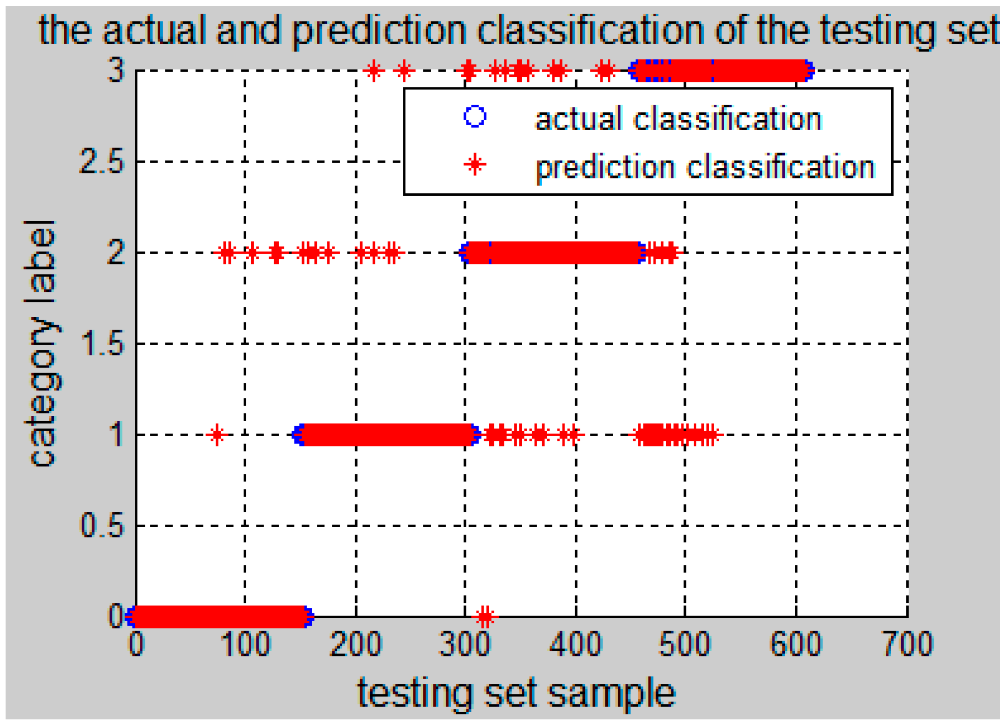
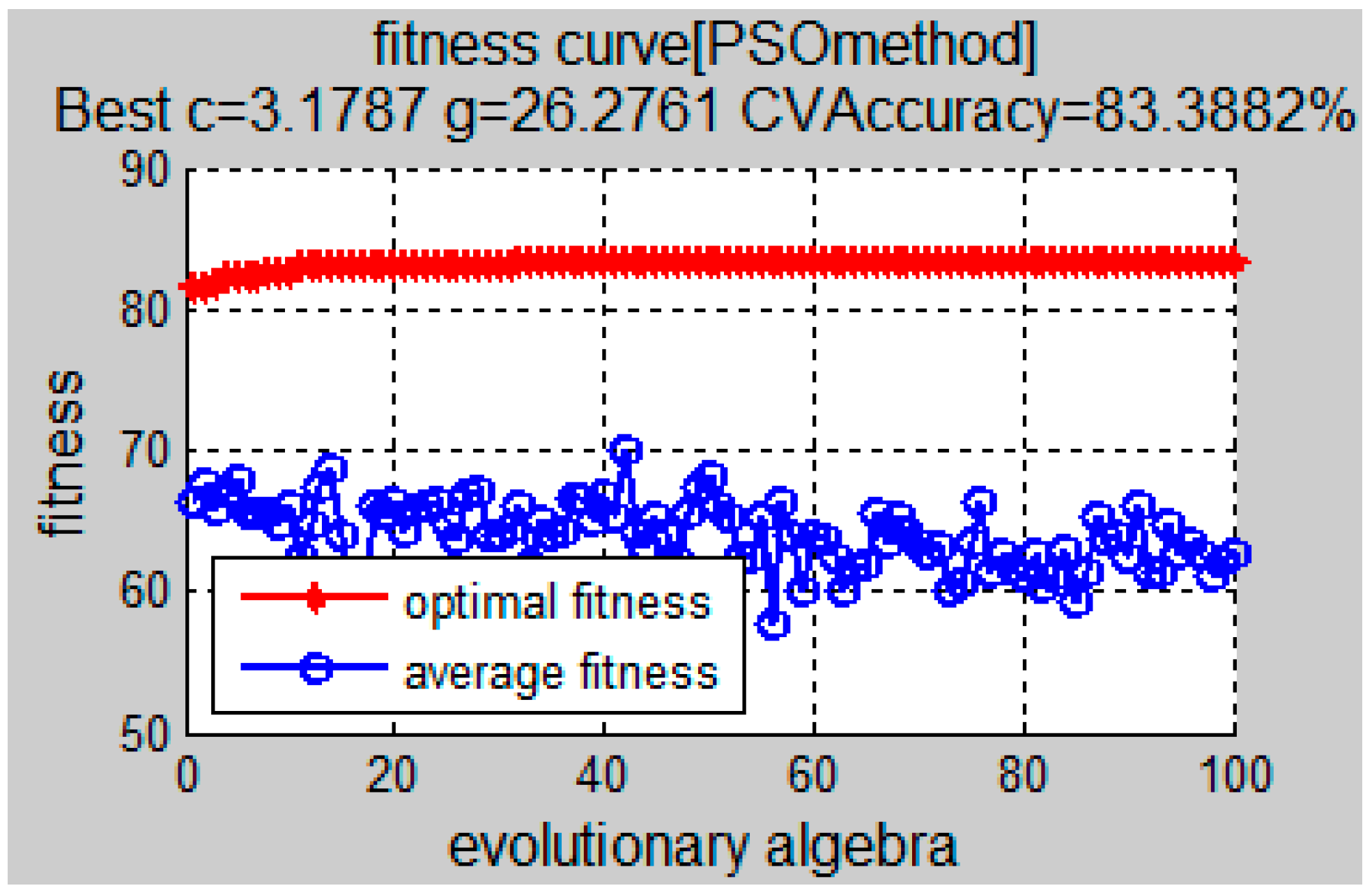
4. PSO-SVM Fault Isolation Results Based on Mixed-Domain Features

The results of parameters optimizing of SVM using PSO and the mixed-domain features of the wind turbine are shown in Figure 3, that is, the optimal fitness of PSO algorithm is 83.3882%, and the obtained optimal parameters are C = 3.1787 , g = 26.2761 . The classification results of the testing set using the optimized SVM classifier are shown in Figure 4, where the category label "0" indicates the normal condition; “1” indicates the parallel misalignment; “2” indicates the angle misalignment; and “3” indicates the comprehensive misalignment.
The classification accuracy rate of training set obtained by using an optimized SVM classifier achieves 97.9441%, and the classification accuracy rate of testing set is 92.1053%, so the fault classification accuracy is very high. In order to better illustrate the superiority of the PSO-SVM algorithm proposed in this paper, the same fault features are adopted by SVM, GridSearch-SVM (the parameters of SVM are optimized by GridSearch) and GA-SVM (the parameters of SVM are optimized by Genetic Algorithm), and the testing results are shown in Figure 5a–c and Table 5.
From the simulation results, it can be seen that the fault isolation by SVM only has a poor recognition effect. When using GridSearch-SVM, the training accuracy and testing accuracy are better, but not higher than PSO-SVM. The training accuracy of GA-SVM is very high, but the promotion ability is less than PSO-SVM. Therefore, it is better to use the PSO-SVM algorithm to isolate the fault.

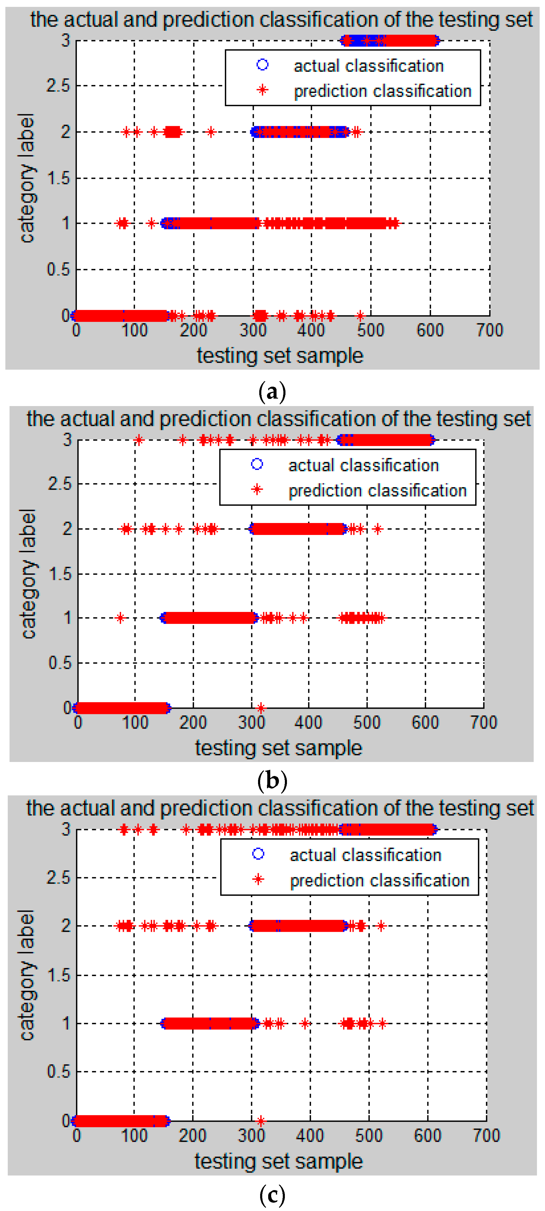
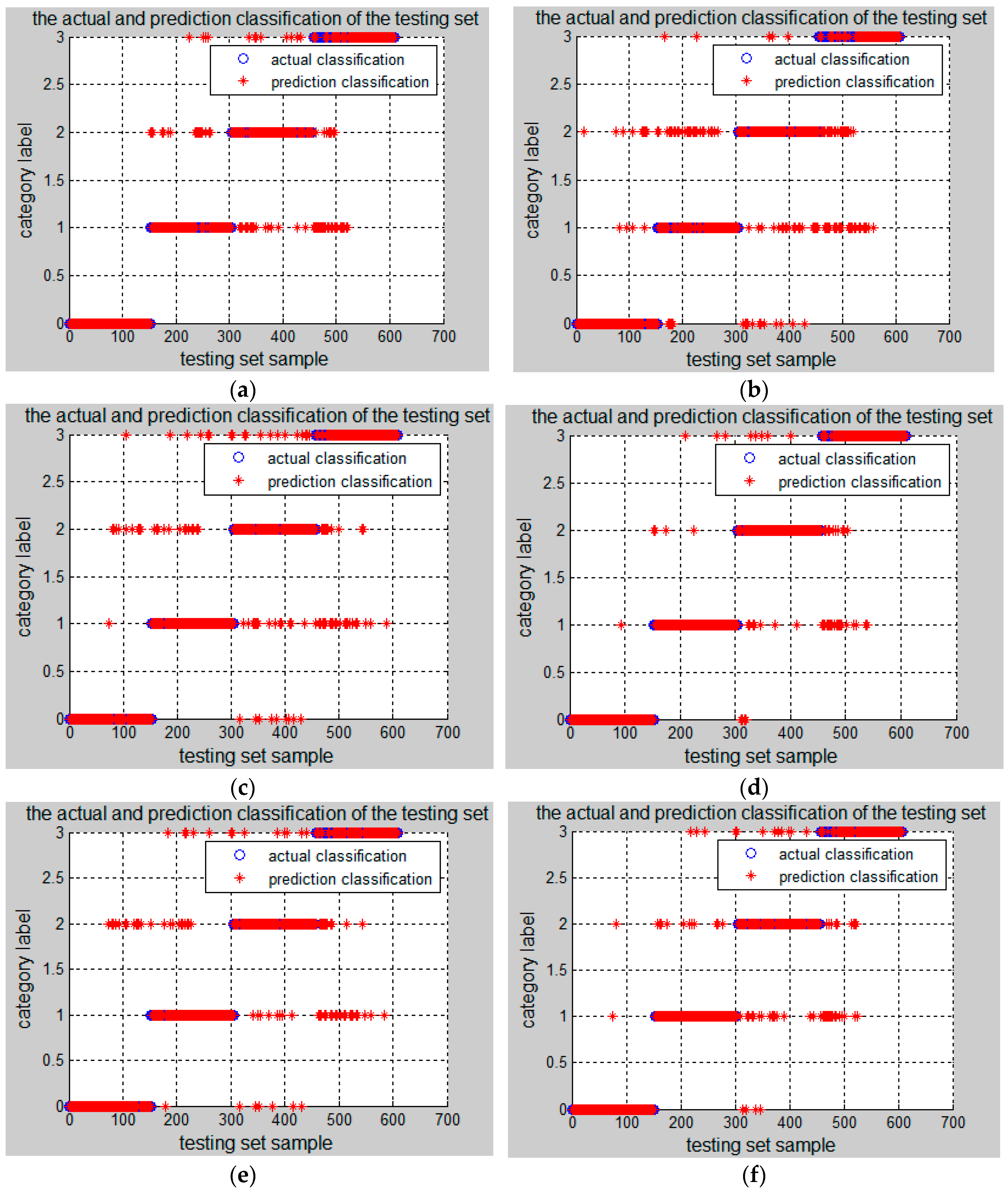
5. Comparison of Fault Isolation Results with Different Fault Features

In this paper, the time-domain, frequency-domain and time-frequency domain features are used to isolation the misalignment fault. In order to compare the superiority of the extracted fault features, the paper also adopts time-domain indexes, frequency-domain indexes, IEMD energy entropy, and their combinations of any two kinds as the inputs of SVM, and the recognition results are shown in Figure 6 and Table 6.
From Figure 6 and Table 6, it can be seen that when the time-domain, frequency-domain and time-frequency domain features are used separately as inputs of the PSO-SVM isolation model, the accuracy of the training set and the testing set are low, and the recognition results are not good. When two kinds of features are combined as the inputs, the training set accuracy is above 91%, the testing set accuracy is more than 84%, and the recognition rate is increased. When the three mixed-domain features are combined, the correct rate of the training set reaches 97.9441%, and the accuracy of the testing set reaches 92.1053%. Therefore, it can be concluded that the mixed-domain features combining three kinds of domain extractions proposed in this paper can effectively reflect the characteristics of the misalignment fault, and can be used to classify the fault types. It is also interesting to note that, whether used individually or combined with energy entropy, the time-domain features seem to provide better identification results than the frequency-domain data. This is because, when the wind turbine transmission system fails, it will produce impact components, and time-domain features can well reflect them, so better results can be obtained when using time-domain features.

6. Conclusions

This paper is based on the time-domain, frequency-domain and time-frequency domain analysis of vibration signals of the wind turbine in four different operating conditions with four kinds of rotating speeds. The mixed-domain features are extracted in the paper, which are the inputs of SVM classifiers. The parameters of SVM are optimized using the PSO algorithm. The testing results show that the proposed model for misalignment fault isolation is effective compared with other commonly used algorithms.
When the wind turbine operates in the condition of misalignment, there will be some changes in the temperature and electrical signals in addition to the reflection of the mechanical aspects, so ANSYS, MATLAB, and other software should be included in the simulation further to get temperature and electrical parameters, so as to study the fault characteristics more comprehensively.
At the same time, it is necessary to point out that the method presented in this paper is a general method, and it can be used elsewhere.

Acknowledgments

This work was supported by the National Natural Science Foundation of China (51577008). The authors are grateful to the anonymous reviewers for their constructive comments on the previous version of the paper.

Author Contributions

Yancai Xiao and Yujia Wang contributed to paper writing and the whole revision process. Huan Mu and Na Kang performed simulation and experiments. All the authors have read and approved the final manuscript.

Conflicts of Interest

The authors declare no conflict of interest.

References

  1. Zhang, T.; Dwight, R.; El-Akruti, K. Condition based maintenance and operation of wind turbines. In Proceedings of the 8th World Congress on Engineering Asset Management & 3rd International Conference on Utility Management & Safety, Hong Kong, China, 30 October–1 November 2013. [Google Scholar]
  2. Zappalá, D.; Tavner, P.J.; Crabtree, C.J.; Sheng, S. Side-band algorithm for automatic wind turbine gearbox fault detection and diagnosis. IET Renew. Power Gener. 2014, 8, 380–389. [Google Scholar] [CrossRef]
  3. Kusiak, A.; Li, W. The prediction and diagnosis of wind turbine faults. Renew. Energy 2011, 36, 16–23. [Google Scholar] [CrossRef]
  4. Bak-Jensen, B.; Kawady, T.A.; Abde1-Rahman, M.H. Coordination between fault-ride-through capability and over-current protection of DFIG generators for wind farms. J. Energy Power Eng. 2010, 4, 20–29. [Google Scholar]
  5. Amirat, Y.; Benbouzid, M.E.H.; Al-Ahmar, E.; Bensaker, B.; Turri, S. A brief status on condition monitoring and fault diagnosis in wind energy conversion systems. Renew. Sustain. Energy Rev. 2009, 13, 2629–2636. [Google Scholar] [CrossRef]
  6. Liao, M.; Liang, Y.; Wang, S.; Wang, Y. Misalignment in Drive Train of Wind Turbines. Mech. Sci. Technol. 2011, 30, 173–180. [Google Scholar]
  7. Xiao, Y.; Kang, N.; Hong, Y.; Zhang, G. Misalignment Fault Diagnosis of DFWT Based on IEMD Energy Entropy and PSO-SVM. Entropy 2017, 19, 6. [Google Scholar] [CrossRef]
  8. Chen, S. Application of Time Domain Analysis in Mechanical Equipment Fault Diagnosis. J. Mech. Transm. 2007, 31, 79–83. [Google Scholar]
  9. Zhen, L. Study on Fault Diagnosis Methods of Generator and Gearbox for Wind Turbines. Master’s Thesis, North China Electric Power University, Beijing, China, 2014. [Google Scholar]
  10. Zhang, C.; Chen, J.; Guo, X. A gear fault diagnosis method based on EMD energy entropy and SVM. J. Vib. Shock 2010, 29, 216–220. [Google Scholar]
  11. Long, J.; Wu, J. Fault Diagnosis of Rotor Misalignment for Windmill Generators. Noise Vib. Control 2013, 33, 222–225. [Google Scholar]
  12. Ding, S.; Chang, X.; Wu, Q.; Wei, H.; Yang, Y. Study on wind turbine gearbox fault diagnosis based on LVQ neural network. Mod. Electron. Tech. 2014, 37, 150–152. [Google Scholar]
  13. Ren, S. The Study of Fault Diagnosis Methods for Wind Turbine Gearbox Based on the Analysis Vibration Characteristics. Master’s Thesis, Hebei University of Technology, Tianjin, China, 2015. [Google Scholar]
  14. Wang, B. Research on Fault Diagnosis System for Gearbox of Wind Turbine. Master’s Thesis, North China Electric Power University, Beijing, China, 2012. [Google Scholar]
  15. Tang, B.; Song, T.; Li, F.; Deng, L. Fault diagnosis for a wind turbine transmission system based on manifold learning and Shannon wavelet support vector machine. Renew. Energy 2014, 62, 1–9. [Google Scholar] [CrossRef]
  16. Li, F.; Tang, B.; Yang, R. Rotating machine fault diagnosis using dimension reduction with linear local tangent space alignment. Measurement 2013, 46, 2525–2539. [Google Scholar] [CrossRef]
  17. Xu, Z. Research on Transmission Chain State Monitoring and Fault Diagnosis of Wind Turbine Based on Vibration Method. Master’s Thesis, Zhejiang University, Hangzhou, China, 2012. [Google Scholar]
  18. Ding, K.; Li, W. Practical Technology for Fault Diagnosis of Gear and Gearbox; China Machine Press: Beijing, China, 2006. [Google Scholar]
  19. Zhang, L.; Zhu, L.; Zhong, B. Study on the Features of Some Specific Parameters Utilized for Machine Condition Monitoring. J. Vib. Shock 2001, 20, 20–21. [Google Scholar]
  20. Yi, L. On-Site Practical Technology of Simple Vibration Diagnosis; China Machine Press: Beijing, China, 2003. [Google Scholar]
  21. Zhang, C.; Chen, J.; Guo, X. Gear fault diagnosis method based on EEMD energy entropy and support vector machine. J. Cent. South Univ. 2012, 3, 932–939. [Google Scholar]
Figure 1. Simplified model of a doubly fed wind turbine.
Algorithms 10 00067 g001
Figure 2. The PSO-SVM fault isolation model.
Algorithms 10 00067 g002
Figure 3. Particle fitness curves.
Algorithms 10 00067 g003
Figure 4. PSO-SVM testing results.
Algorithms 10 00067 g004
Figure 5. Fault isolation results of other algorithms. (a) SVM testing results; (b) GridSearch-SVM testing results; (c) GA-SVM testing results.
Algorithms 10 00067 g005
Figure 6. Testing results of PSO-SVM using different input features. (a) using time-domain features only; (b) using frequency-domain features only; (c) using IEMD energy entropy features only; (d) using time-domain + frequency-domain features; (e) using frequency-domain + IEMD energy entropy features; and (f) using time-domain + IEMD energy entropy features.
Algorithms 10 00067 g006
Table 1. Mixed-domain feature library.
Feature LibraryFeatureIndex
Mixed-domain feature libraryTime-domainroot mean square, square root amplitude, variance, standard deviation, kurtosis, waveform index, peak index, pulse index, margin index, kurtosis index
Frequency-domaincentroid frequency, mean square frequency, variance frequency
Time-frequency domainenergy entropy of the first eight IMF components of IEMD decomposition
Table 2. The partial data of the time-domain indexes.
TypeRMS (×10)Square Root AmplitudeVariance (×106)SD (×10)KurtosisWaveform IndexPeak IndexPulse IndexMargin IndexKurtosis Index
010,10771,06910,21210,1052.491.213.424.154.862.50
10,11270,65110,22310,1112.531.223.023.684.322.54
10,11769,92010,22910,1142.551.223.284.014.742.56
10,13570,62710,26110,1302.521.223.444.194.932.54
10,13669,84410,26710,1322.591.233.033.724.402.60
168,743203,77047,18468,69014.191.896.2611.8121.1114.40
70,048213,12049,04670,03315.371.855.4410.0717.8915.51
70,194208,35049,20970,14914.691.905.219.9017.5714.94
70,720217,07049,93170,66216.041.915.119.7516.6616.30
71,651227,77051,20171,55512.081.845.5710.2417.5312.23
2176,820689,72030,935175,8807.411.644.427.2411.347.58
177,180702,01031,389177,1706.721.634.877.9212.286.72
177,930680,85031,660177,9307.521.674.788.0012.507.52
178,990679,15031,589177,7307.711.693.846.4810.138.28
179,010706,13032,048179,0206.771.645.048.2612.776.77
3601,3601,681,90036,139601,16014.831.955.8211.3520.8115.09
625,9101,801,80039,127625,52013.281.916.7012.7623.2613.58
656,9702,154,20043,123656,68011.111.797.3013.0922.2711.22
664,8602,069,30044,194664,78011.381.826.8012.3721.8511.51
671,7502,101,20045,063671,29012.301.836.8212.5021.8112.50
Table 3. The partial data of the frequency-domain indexes.
TypeFCMSFVF
0−4587,083,8006,873,700
−4557,047,8006,841,100
−4577,077,4006,868,500
−4536,958,7006,753,100
−4486,988,7006,787,900
1−75012,950,00012,387,000
−64711,048,00010,629,000
−69712,436,00011,950,000
−72813,462,00012,933,000
−71512,794,00012,283,000
2−4408,587,500 8,393,500
−4438,652,700 8,456,200
−4759,280,300 9,053,800
−4478,707,000 8,507,200
−4518,785,300 8,581,700
3−3767,338,600 7,196,600
−3557,033,700 6,907,400
−3888,190,100 8,039,200
−3697,400,400 7,264,100
−3466,958,600 6,838,700
Table 4. The partial data of the energy entropy of the first eight IMF components of IEMD.
Type P 1 P 2 P 3 P 4 P 5 P 7 P 7 P 8
00.31090.34290.17090.07470.04760.0720.0970.0521
0.31660.3520.15530.07840.04770.06880.05750.0176
0.31860.34980.16570.08140.04780.04520.0690.0172
0.32560.3410.20310.08950.05640.0370.09330.0148
0.33020.33860.16690.07480.05740.05220.07880.0129
10.14840.36760.36230.1930.12010.08630.04770.1012
0.14890.36690.36780.22670.09380.04810.0280.1249
0.15130.36780.36620.18390.10770.06650.05170.2216
0.15580.35330.36750.21330.14790.06830.06370.1977
0.15740.36010.36390.1570.08070.0620.20310.1429
20.23350.30670.23250.14670.08430.07630.13860.3648
0.23610.30240.36790.2890.19340.11570.15940.0478
0.24230.36650.34170.25740.18620.08970.03950.0279
0.24550.34760.36790.30960.10830.08730.03370.0536
0.24870.32980.31340.25650.12540.08040.13090.3447
30.14560.22850.29120.33220.25210.16720.20010.1162
0.10610.27840.33930.28760.27620.08130.20590.1677
0.10740.25810.33570.35820.16060.11010.13960.1396
0.10820.28530.32710.30220.16850.17650.07510.1556
0.1110.32680.36540.27370.26810.08860.07730.1014
Table 5. Comparison of PSO-SVM with other commonly used classifiers.
Item C g Accuracy of Training SetAccuracy of Testing Set
SVM10.0163.2401% (769/1216)63.6513% (387/608)
GridSearch-SVM161.414293.4211% (1136/1216)90.9539% (553/608)
GA-SVM26.21686.716299.5066% (1210/1216)91.1184% (554/608)
PSO-SVM3.178726.276197.9441% (1191/1216)92.1053% (560/608)
Table 6. PSO-SVM classification results of different fault features.
Fault Features C g Accuracy of Training SetAccuracy of Testing Set
Time-domain22.539674.882388.0757% (1071/1216)84.2105% (512/608)
Frequency-domain7.71812346.31677.7138% (945/1216)74.5066% (453/608)
IEMD energy entropy7.885736.1241487.4178% (1063/1216)82.4013% (501/608)
Time-domain + frequency-domain73.078620.028193.5033% (1137/1216)89.9671% (547/608)
Time-domain + IEMD energy entropy58.31061.4290493.2566% (1134/1216)87.8289% (534/608)
Frequency-domain + IEMD energy entropy2.109310.023191.1184% (1108/1216)84.8684% (516/608)
Time-domain + frequency-domain + IEMD energy entropy3.178726.276197.9441% (1191/1216)92.1053% (560/608)

