A New Approach to Image-Based Estimation of Food Volume

Abstract

A balanced diet is the key to a healthy lifestyle and is crucial for preventing or dealing with many chronic diseases such as diabetes and obesity. Therefore, monitoring diet can be an effective way of improving people’s health. However, manual reporting of food intake has been shown to be inaccurate and often impractical. This paper presents a new approach to food intake quantity estimation using image-based modeling. The modeling method consists of three steps: firstly, a short video of the food is taken by the user’s smartphone. From such a video, six frames are selected based on the pictures’ viewpoints as determined by the smartphone’s orientation sensors. Secondly, the user marks one of the frames to seed an interactive segmentation algorithm. Segmentation is based on a Gaussian Mixture Model alongside the graph-cut algorithm. Finally, a customized image-based modeling algorithm generates a point-cloud to model the food. At the same time, a stochastic object-detection method locates a checkerboard used as size/ground reference. The modeling algorithm is optimized such that the use of six input images still results in an acceptable computation cost. In our evaluation procedure, we achieved an average accuracy of $92\%$ on a test set that includes images of different kinds of pasta and bread, with an average processing time of about 23 s.

1. Introduction

People’s eating behavior has been shown to affect health issues [1]. This fact has fostered the emergence of many approaches to monitoring diet whose targets include the food items comprised in each meal, as well as the general eating habits of a person. However, most currently used self-reporting techniques generally cause an underestimation of food intake, related with diverse psychological implications [2]. While such an attitude is rather obvious in people overweight, under-reporting of dietary energy intake has been shown to be common even in non-obese adults [3]. Another relevant problem is the different degree of motivation with which individuals fill the reports. Differences relate to factors like awareness of food intake (particularly with snacks), literacy level, and memory and perception capabilities [4].

Thus, self-reported food intake data should be interpreted with caution unless their validity is assessed by independent methods [3]. Because of this, many researchers have started developing affordable non-invasive automatic solutions that help users measure and analyze their food intake [5].

Estimating the size or volume of food items, once the food type is known, is the most direct way of estimating the nutrition properties of the food pictured in an image.

Several methods try to estimate food size from a single image. Martin et al. assume that a correlation exists between the area of the region where food is visible in an image and its actual volume [6]. To achieve the same goal, the system described in [7] first detects the camera pose using a fiducial marker placed within the scene and then tries to match the food item by generating several pre-defined 3D shape models of which the best-matching one is adopted. However, this approach works only for the items that can be approximated by the regular shapes it takes into consideration.

Many studies have tried to use more than one image to overcome the problems related with the lack of depth information in two-dimensional images and with occlusions that may hide some objects. In [8], two images provide the top and side views of the dish. In [9], the user takes three pictures from which the system computes a dense 3D point-cloud including all points on the dish and then estimates the volume using Delaunay triangulation. Dehais et al. [10] also suggest a computationally affordable method for volume estimation based on a dense 3D point-cloud.

In our previous work, we developed two of the basic modules needed to accomplish food volume estimation. In [11], we proposed an interactive segmentation solution for smartphones, which provided a robust and highly accurate approach to segmentation in spite of its simplicity and practicality. In [12], we designed a quick and accurate stochastic model-based solution for locating small checkerboards to be used as size references within an image.

In this work, we introduce a complete solution to estimate food item volume based on a short video. It integrates our previously-developed methods with a new approach to image acquisition and image-based modeling. This end-to-end solution is designed to be usable in practical food intake monitoring solutions. We first describe the method, which is composed of four main steps: acquisition, segmentation, size/ground reference detection, and modeling. Then, we discuss the evaluation procedure and the results we obtained on a test set that includes images of different food items.

2. Method

The system has been designed as a client-server solution. The smartphone acts as the client and runs the semi-automatic part of the system. Building on our previous work, we complete the processing cycle addressing all of the main practical and theoretical issues related with food volume estimation.

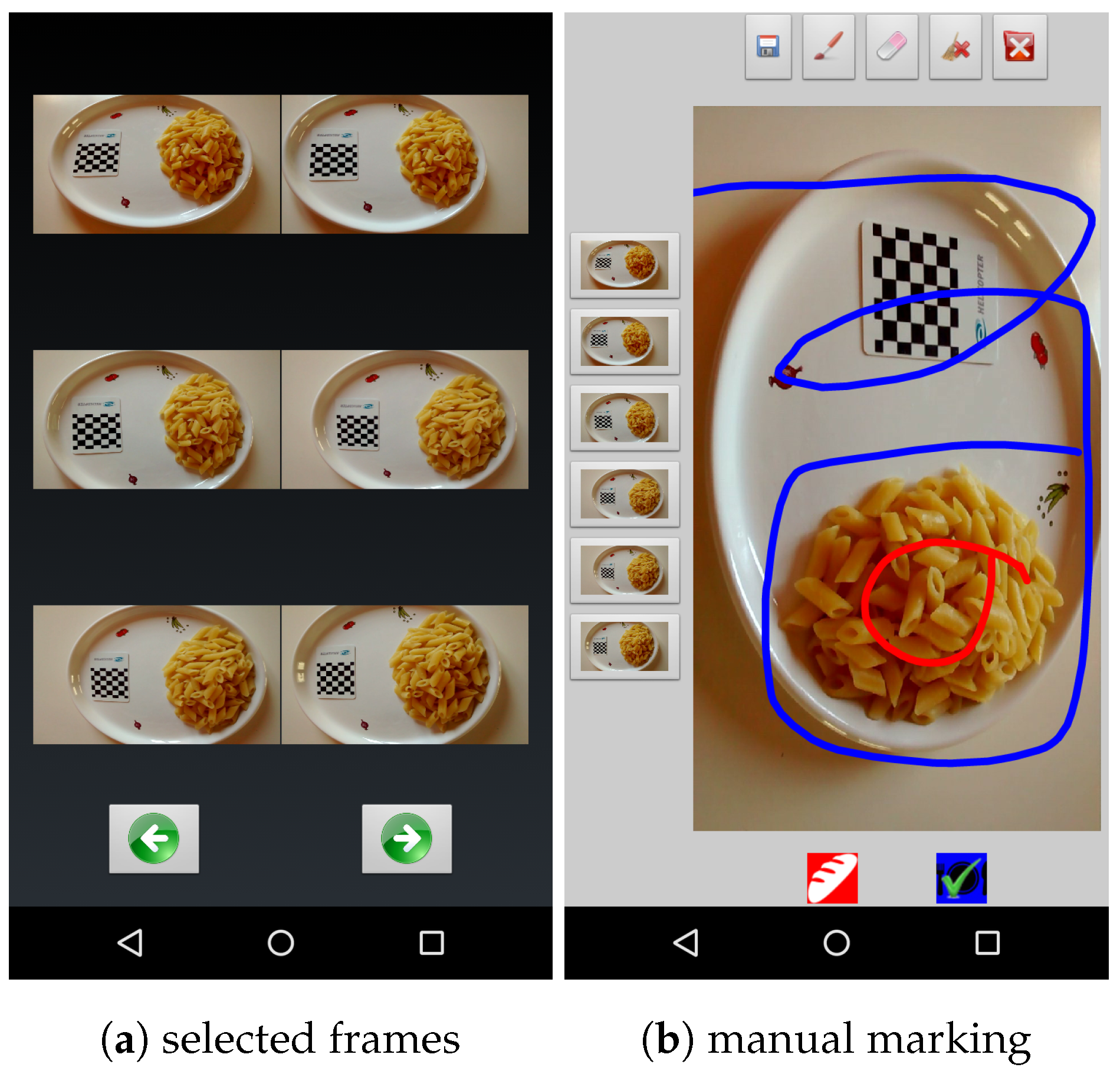
In the system described in this paper, as a first step, the user is asked to take a short video of the food. Then, a subset of the frames is automatically extracted from the video to provide relevant views of the food from all sides. Next, the user marks some food and non-food parts in one of the selected frames of the video. A mobile application that we developed facilitates this part (see Figure 1). The segmentation process, which is performed on the server side, is seeded by the user’s marks. The segmented images are then fed into a customized image-based process that builds a 3D model of the food items. This model is finally used to calculate the volume of the food. A small checkerboard is used as the size and ground reference for the modeling process.

2.1. Image Acquisition

Reconstructing the 3D model of an object from a set of input images requires the availability of relevant visual information about the whole object. Usually, as happens in [9,10], the reconstruction is based on two or three images taken from different viewpoints. The main problem with these approaches is that such a small number of images is usually not enough to acquire the necessary information from all sides of objects and may lead to an incomplete reconstruction. This problem is particularly relevant for methods that include steps, like feature matching or fundamental-matrix estimation, which are very sensitive to noise or lack of information.

Thus, our method relies on information drawn from a larger number of images to obtain a better coverage of the whole object. This also allows it to achieve satisfying results using relatively low-resolution images.

Acquiring a larger number of images is usually avoided because, in that situation, the user should be skilled enough to choose the best viewpoints, while the goal of the app is to limit user intervention at most to a few purely mechanical gestures that do not require any problem-specific knowledge. In our approach, the user takes a short video of the object by moving the camera around it for a few seconds to make sure that images of the object are acquired from virtually all possible viewpoints. Then, the application automatically selects six frames that optimize object coverage based on the orientation of the smartphone during filming. The frame selection process is performed almost in real time, so one can use the application smoothly. Figure 2 provides an example of the output of this step, showing the six viewpoints that have been automatically selected by the application.

The built-in sensors of the mobile device are used for the selection process. Most modern smartphones are equipped with different kinds of sensors, among which accelerometer and geomagnetic field sensors are very common. These sensors can provide enough data to detect the orientation of the smartphone in each moment. The orientation of the device is defined by three values (pitch, roll, and azimuth), which, respectively, correspond to the rotation angles around the x-axis, y-axis, and z-axis. The application records the time-tag of the frames that coincide with the min/max values of pitch, roll, and azimuth recorded while taking the movie. Algorithm 1 reports the pseudo code of the function used to detect the proper frames. Later, six frames presenting the min/max rotational moments are chosen as the input of the modeling process. Thus, the user neither needs to take several images nor should worry about choosing proper camera viewpoints. Moreover, the Graphical User Interface (GUI) of the app allows the user to remove one of the images or to replace it with some other frame just by tapping on the screen. Figure 1 shows two snapshots of the mobile application.

Algorithm 1 Choosing six frames to obtain a good coverage of the object

function onSensorChanged(SensorEvent event)     if event.sensors include [ACCELEROMETER, MAGNETIC_ FIELD] then         $pitch,roll,azimuth\leftarrow SensorManager.getOrientation\left(\right)$         if pitch is new min/max then            $RememberTimeTag\left(\right)$         end if         if roll is new min/max then            $RememberTimeTag\left(\right)$         end if         if azimuth is new min/max then            $RememberTimeTag\left(\right)$         end if     end if  end function

2.2. Segmentation

The objective of the segmentation step is to detect the exact location of the food items in the images. Food image segmentation can be very challenging. There are very different ways of cooking the same kind of food and of arranging food on a dish. These problems and many other factors cause food appearance to vary dramatically. Some studies impose constraints when taking pictures of food, in order to make segmentation easier. For example, Zhu [13] assumes that food lies on a dish that is brighter than the table cloth. Several other studies [14,15,16] impose that the dish, or the container where the food lies, has a pre-specified shape.

Recently, attention has been paid to semi-automatic methods. In [17,18], the user is requested to draw a bounding box around the food items, while in [19], the user must mark the initial seeds before starting to grow segments. In this work, a semi-automatic method is designed which can be run on smartphones in a user-friendly manner.

The method is based on a customized interactive version of the graph-cut (GC) algorithm [20], which deals with image segmentation as a pixel-labeling problem. The graph-cut algorithm assigns a “foreground” (food) or “background” (not food) label to each pixel.

We evaluated the general effectiveness of this method in a previous work [11]. In our customized version of GC, the user imposes some hard constraints by marking some food and non-food areas in one of the images. The application provides a user-friendly environment for marking images by simply touching the screen (see Figure 1).

Algorithm 2 reports the pseudo-code of this process. The marked parts of the image are fed into a Gaussian Mixture Model (GMM) algorithm [21] that estimates the distribution of the Red-Green-Blue (RGB) values for the image foreground (food) and background (not food). The K-means algorithm is then used to divide the data from each RGB channel into ten clusters that are assumed to follow a normal distribution. Then, the GMM estimates the distribution by combining the normal models. Next, a value is assigned to every pixel, which denotes the likelihood of its belonging to the foreground or the background, based on the distribution estimated by the GMM. These likelihood values are used to seed the graph-cut algorithm, which produces the final segmentation. However, if the user is dissatisfied with the segmentation output, he/she can repeat the marking step to improve the result.

Algorithm 2 Segmentation of a marked image using GMM and graph-cut

function Segmentation(OriginalImage, MarkedImage)     $Pixel{s}_F\leftarrow \mathbf{ExtractFoodPixels}(OriginalImage,MarkedImage)$     $Pixel{s}_B\leftarrow \mathbf{ExtractBackgroundPixels}(OriginalImage,MarkedImage)$     $GM{M}_F\leftarrow \mathbf{ComputeFoodGMM}\left(Pixel{s}_F\right)$     $GM{M}_B\leftarrow \mathbf{ComputeBackgroundGMM}\left(Pixel{s}_B\right)$     $Lik{e}_F\leftarrow \mathbf{CalcFoodLikelihood}(OriginalImage,GM{M}_F)$     $Lik{e}_B\leftarrow \mathbf{CalcBackgroundLikelihood}(OriginalImage,GM{M}_B)$     $Segments\leftarrow \mathbf{GraphCut}(Lik{e}_F,Lik{e}_B)$ return Segments end function

Although the input to the segmentation method we propose consists of the six images which are automatically extracted from the short video, the user needs to mark only one of them. The segmentation for such an image obtained based on the marked pixels is then used to extend the process to the other images by recomputing the GMM on the whole segmented image and using such a more accurate estimate as the model used in segmenting the others. This is based on the primary assumption that the images acquired are characterized by a similar color distribution. 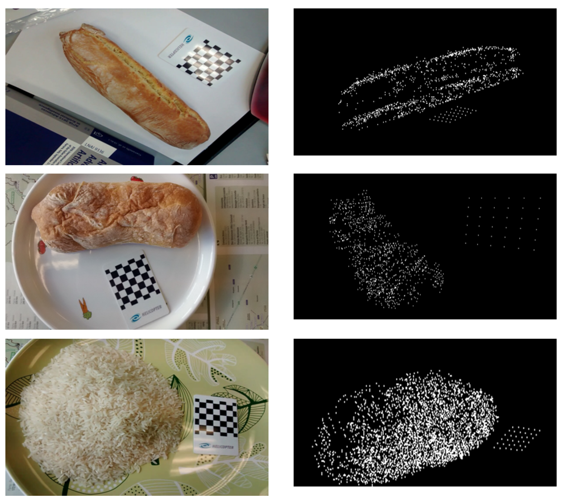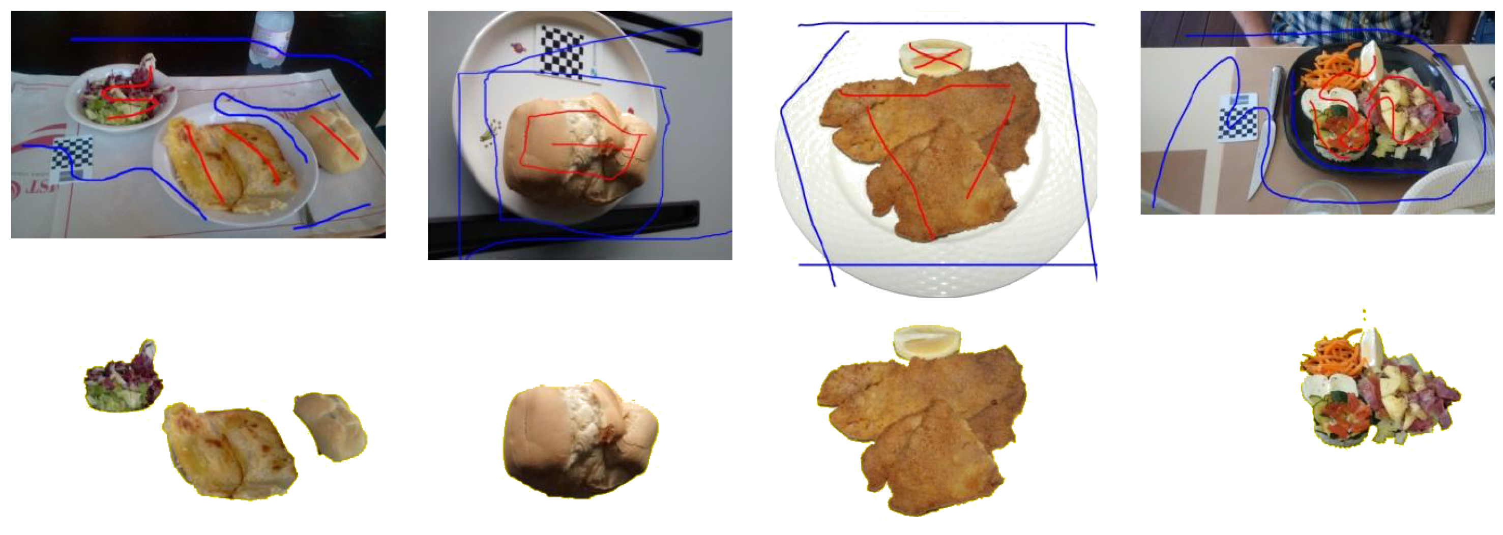Figure 3 shows the segmentation of four food images obtained by our method.

Being based on six images, a small segmentation error in one image can be recovered by the results obtained on the other images. In fact, if the errors are not very large, the object part corresponding to an under/over-segmentation of one item might be correctly segmented in others. This gives more flexibility to the method and minimizes processing time because every part needs to be marked as the foreground in at least two images to be taken into consideration in the modeling process.

2.3. Size/Ground Reference Localization

Volume can be estimated from images using several different procedures, but results are computed only up to a scale factor. Therefore, in many studies, an object of known size is used as a reference for volume estimation. In [8], for instance, the user puts his/her finger besides the dish. In [6], a specific pattern of known size printed on a card is used as a reference. 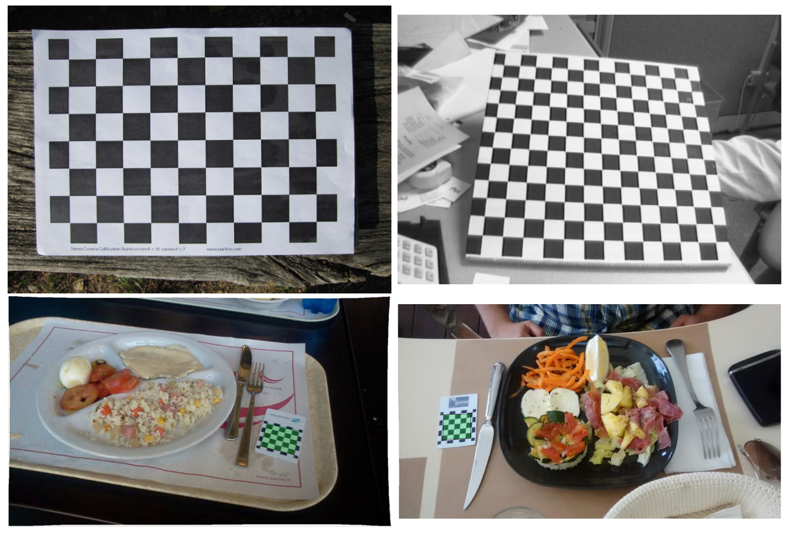Many studies have followed the same idea using a checkerboard as a reference [13,22] because of the simplicity of the checkerboard pattern and the existence of effective algorithms to detect it. Nevertheless, off-the-shelf checkerboard detection algorithms are usually designed to be means for camera calibration or pose-detection processes. They are usually tuned for specific situations like: flat checkerboards, a big checkerboard that is often the only object in the image, etc. Thus, for applications that do not satisfy these requirements, different algorithms, or modified versions of available ones, are needed. Checkerboards that are used as size references usually consist of few squares and occupy a relatively small region of the image. This makes detecting them hard for ‘standard’ checkerboard detectors. Figure 4 shows three examples in which the checkerboard detection algorithms provided by the open software package OpenCV 3.1.0 [23] and Matlab R2014b (The MathWorks Inc., Natick, MA, USA) fail.

In [12], we have introduced a method to locate a small checkerboard in an image. We used a $5\times 5$ checkerboard, printed on a Polyvinyl Chloride (PVC) card, as a size reference. The method consists of two main steps: locating the checkerboard in the image and then detecting the checkerboard corners in the located area.

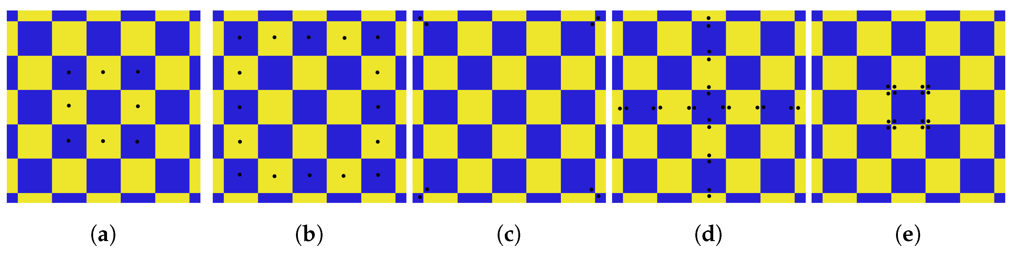
The procedure that we adopt estimates the pose of an object based on a 3D model and can be utilized with any projection system and any general object model. Figure 5 shows the model that we use to detect the checkerboard. It consists of 73 key points corresponding to the center, edges and corners of each square.

In this method, a hypothesis of checkerboard location can be evaluated by rigidly transforming a model of the checkerboard and then projecting it onto the image according to a perspective transform. The likelihood of the hypothesis is evaluated using a similarity measure between the projected model and the actual content of the image region onto which the pattern is projected.

This procedure allows one to turn checkerboard detection into an optimization problem, in which the parameters to be optimized are the coefficients of the rigid transformation and of the projection. In this work, Differential Evolution (DE) [24] is employed for optimization as described in [25]. Algorithm 3 reports the pseudo-code of the fitness function used to evaluate each hypothesis. In the algorithm, each step presented in Figure 5 is implemented as a separate function. One of the advantages of using a stochastic algorithm like DE is having a chance of success in the next try if an attempt to find the checkerboard fails.

Algorithm 3 Fitness Function

function FitnessFunction(PoseVector)     Calc Rotation & Translation matrices from PoseVector     $Score\leftarrow Score+FirstLevelCenterCheck\left(\right)$     if Score > 6 then         $Score\leftarrow Score+SecondLevelCenterCheck\left(\right)$     end if     if Score $>20$ & the center is black then         $Score\leftarrow Score+PoseCheck\left(\right)$     end if     if Score > 23 then         $Score\leftarrow Score+EdgesCheck\left(\right)$         $Score\leftarrow Score+VerticesCheck\left(\right)$     end if return Score end function

Based on this estimated checkerboard location, the corners of the checkerboard are then precisely detected as described in [12]. This allows the algorithm to estimate the checker size and, consequently, the scale factor, which is to be applied to estimate food volume.

Additionally, the checkerboard can be assumed as a reference for the ground surface, whose orientation is represented by the plane having the smallest squared distance from the checkerboard corners.

If we term n the vector normal to the ground plane and $P=[p_1,...,p_n]$ a $3\times n$ matrix in which the columns are the detected corners’ coordinates, the plane can be found by calculating the Singular Value Decomposition (SVD) of $A=[p_1-c,p_2-c,....,p_n-c]$, where c is a point belonging the plane [26]. We set c equal to the centroid of the columns of P and set n as the left singular vector of the SVD [26].

This use of the checkerboard is valuable during 3D-modeling to extract more information about the lower parts of the object, which could be invisible in the video taken from above, as well as to remove noise.

The approach requires that the checkerboard be at the same height as the food, which might raise some concerns about the practicality of the method. However, the procedure could still be useful, especially since one can estimate the average thickness of the dishes where users commonly eat and print the pattern on top of a box, in order to lift it at more or less the same level and compensate for the thickness of the dish. The use of the checkerboard as ground-reference mainly helps to eliminate noise and outliers from the model’s point-cloud. These outliers are usually located below the surface, at a very large distance from it. Therefore, the method only requires that the checkerboard be ’almost’ on the same level as the dish bottom surface.

2.4. Image-Based Modeling

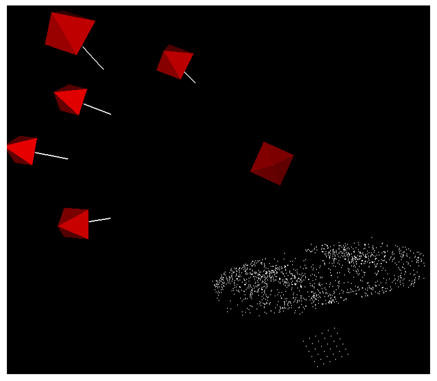
In this step, a 3D model of the food item in the form of a point-cloud is generated based on a Structure from Motion (SfM) algorithm. We followed the same approach described in [27,28], properly adapting it to this work. In fact, the base approaches have been designed to build a model based on many (up to a few thousands) images. Our algorithm is customized for using a lower number of images (six, in our case) and address processing time-related concerns. Algorithm 4 reports the pseudo-code of the method, while Figure 6 shows three examples of the reconstructed models.

Algorithm 4 3D modeling algorithm

function Model(OriginalImages[], SegmentedImages[], CameraMatrix)

▹ Prepare Matches

$Matches\left[\right]\leftarrow \mathbf{Extract}-\mathbf{SURF}-\mathbf{BRISK}-\mathbf{Matches}\left(OriginalImages\right[\left]\right)$     $Matches\left[\right]\leftarrow \mathbf{PruneOutliers}\left(Matches\right[\left]\right)$

▹ Start Modeling

$BaseLine\leftarrow \mathbf{FindTheBestPair}\left(Matches\right[\left]\right)$     $PointCloud\leftarrow \mathbf{Triangulate}(BaseLine,Matches[],CameraMatrix)$     while there is more un-processed image do         $NextImage\leftarrow \mathbf{ChooseNextImage}(PointCloud,Matches[\left]\right)$         $NewMatrix\leftarrow \mathbf{FindPoseAndCameraMatrix}(PointCloud,Matches[],CameraMatrix)$         $PointCloud\leftarrow PointCloud+\mathbf{Triangulate}(BaseLine,Matches[],NewMatrix)$     end while

▹ Find Checkerboard

$Corners\leftarrow \mathbf{FindCheckerboardCorners}\left(OriginalImages\right[],CameraMatrix)$     $Scale\leftarrow \mathbf{EstimateSizeScale}\left(Corners\right)$     $SurfacePlane\leftarrow \mathbf{EstimateSurfacePlane}\left(Corners\right)$

▹ Refine PointCloud

$PointCloud\leftarrow \mathbf{EliminateNoise}(PointCloud,SurfacePlane)$ return PointCloud, Scale end function

First, Speeded Up Robust Features (SURF) [29] of the images are extracted and their Binary Robust Invariant Scalable Keypoints (BRISK) [30] description is used to find matches between image pairs. A pair is considered to be relevant if it produces at least 30 matches, in which case the corresponding points are added to the point-cloud. There are 15 possible pairs in total to be taken into consideration for six images, which is generally a large number, which could affect the total processing time significantly. Therefore, only a limited number of image pairs, configurable by the user, are actually used instead of all possible pairs.

Then, the Fundamental Matrix [31] is calculated for all image pairs using an 8-point Random Sample Consensus (RANSAC) [32]. The RANSAC outliers threshold is set to $0.6\%$ of the maximum image dimension (i.e., the largest between height and width) and the level of confidence is set to $99\%$. The results of RANSAC are therefore also used to “clean” the point-cloud by removing outliers.

In the next step, the best image pair is chosen as the starting point for the 3D reconstruction, using the results of a homographic transformation as a selection criterion. Homography is the mathematical term for mapping points on one surface to points on another. The transformation between images of each pair is calculated using the RANSAC with the outliers threshold set to $0.4\%$ of the largest image dimension. This method, besides finding the transformation, classifies the matching features into inliers and outliers. The pair with the largest inlier rate is chosen to start the reconstruction. The quality of the selected image pair is further evaluated by checking the validity of its Essential Matrix [31]. If the selected pair fails the test, the next best pair is chosen as the baseline of the 3D reconstruction.

Then, the 2D coordinates of the matching points belonging to the selected images are used to calculate the corresponding 3D coordinates. Assuming $P_i$ to be the camera matrix of the $i^{th}$ image and $x_i$ and $x_j$ the 2D coordinates of two matching points in the $i^{th}$ and $j^{th}$ image, the relationships $x_i=P_{i}X$ and $x_j=P_{j}X$ hold, where X denotes the 3D coordinate of the projected point. Moreover, for every point that is not too close to the camera or at infinity, one can say $X=(x,y,z,1)t$, where t is the scaling factor. This creates an inhomogeneous linear system of the form $AX=B$. The least-squares solution of this equation can be found by using the Singular Value Decomposition (SVD). Unfortunately, this method is not very accurate. The method introduced by Hartley and Sturm [33] iteratively re-calculates X by updating A and B based on the results of the previous step. This allows one to refine the estimate and to significantly increase accuracy.

The other images are then successively taken into consideration in the triangulation process. Since the 3D coordinates can be estimated only up to a scaling factor t, the 3D points belonging to different image pairs might have a different scale factor, and it may be therefore impossible to build a consistent 3D reconstruction. The other issue is the order in which the different views are taken into account. Taking into account a lower image-quality view before the others may affect the final model negatively. In order to tackle these issues, we first choose the best view among the remaining ones by calculating, for each view, the number of features that produce successful matches with the images that have been previously processed, and selecting the one for which it is largest. Then, the camera position for the selected view is estimated based on the previously reconstructed points. This is a classic Perspective-n-Point problem (PnP), which determines the position and orientation of a camera given its intrinsic parameters and a set of n correspondences between 3D points and their 2D projections. The $solvePnPRansac$ function, provided by OpenCV, which finds the pose that minimizes the reprojection error, is used to solve it. The use of RANSAC makes the function robust to outliers. This approach also ensures that the 3D points added to the point-cloud based on the new images share the same scaling factor as the previous ones.

Bundle Adjustment [34] is also applied to the triangulation output in order to refine the results. It is an optimization step that provides a maximum-likelihood estimation of the positions of both the 3D points and the cameras [34]. This result is obtained by finding the parameters of the camera view $P_k$ and the 3D points $X_i$, which minimize the reprojection error, i.e., the sum of squared distances between the observed image points $x_{ki}$ and the reprojected image points $P_k\left(X_i\right)$ [31].

In the next step, all of the non-object points are removed from the point-cloud based on the output of the segmentation stage. The requirement by which a 3D point must appear in at least two images compensates for some segmentation errors that might have occurred in some images.

Finally, outliers are removed from the point-cloud. Since the ground surface has been determined based on the checkerboard location, it is possible to apply restrictions to the maximum acceptable height of the food item (we set such limit to 20 cm). The point-cloud usually also includes isolated outliers that are relevantly far from the other points. To deal with this problem, we remove from the point-cloud the points whose distance from the closest neighbor is larger than a threshold. In practice, for each point, four types of distances are defined: the Euclidean distance and the distances along the three coordinate axes. Acceptable points should be no farther from their nearest neighbor than one standard deviation for each of the measures taken into consideration.

Moreover, if an isolated set of less than five points is too far from its neighbors, it will be removed as well.

3. System Evaluation

We have already evaluated the segmentation algorithm as well as the checkerboard detection method that we use to set a size reference separately in our previous works, where we introduced such approaches [11,12]. In this work, we completed the system and could finally evaluate the accuracy of our solution for estimating an object’s volume.

The main objective of the study was to establish a robust and consistent method to estimate food volume. This means that, first, the method should estimate the same volume for the same amount of food in different dishes. Then, the method should present a steady correlation between food amount and estimated volume when one changes the amount of food. If the algorithm is able to produce a result correlated with the actual food amount, it could later be translated into a good estimation of the actual nutrition facts of the food.

We evaluated the method using two common types of food items: food items with a solid shape and food with non-solid shapes. In both procedures, we assumed that the shapes were more or less convex, in order to keep the volume estimation simple. Thus, it was possible to estimate the volume of the models that we generated using the Qhull tools [35]. Furthermore, for each test case, we ran the whole procedure twice to have more reliable results. All of the tests were performed on a PC equipped with an Intel^® Core™$i7$ 2.8 GHz CPU and running the 64-bit version of Windows 7 Professional (Microsoft Corporation Redmond, WA, USA).

For the first group, six types of bread were chosen as the test cases. Since we took convex objects into consideration, in this case, our goal was to evaluate the accuracy of the reconstructed shape. In order to establish a precise ground truth, we used an industrial 3D laser scanner Sick LMS400 (SICK AG, Waldkirch, Germany) to acquire as accurate a 3D model of the test objects as possible. The device has a spatial resolution of 1 mm and the scanned model was manually segmented to acquire a more accurate ground truth.

Table 1. Error rate in the reconstructed models’ volume estimations for solid shapes.

Row	Bread	Error (%)
1		$7.2\%$
2		$4.9\%$
3		$9.5\%$
4		$1.7\%$
5		$19.1\%$
6		$7.2\%$
	average	$8.27\%$
	average processing time	21.5 s

shows the results obtained on the first group of food items (different sorts of bread). The average error rate of the whole process (including acquisition, view selection, segmentation, size reference detection, and 3D model reconstruction) over all cases was $8.27\%$. As shown in Table 1, the error rate for item number 5 is larger than for the other items due to its poor visual context. In fact, it has a smoother surface showing small variations of shade and color, which allows one to extract only few relevant features. The error on item number 6 is also higher than expected, despite its rich visual context. This appears to be a consequence of its small size, which increases the relative weight of noise.

The average processing time on this first test set, including the whole process from segmentation to volume estimation, was around 21 s.

In the second part, we made tests with pasta and rice as examples of food with non-solid shapes. Two types of evaluations were made on this test set. First, in order to assess the stability of the method, we made several independent tests with the same amount of the same kind of food. For example, for each type of pasta, the same amount of raw pasta was cooked and tested on two different dishes. In addition, for each dish, the test was repeated with a different layout as well (in total, four times for the same amount of pasta). As a second evaluation, we tested the correlation between the actual food weight and the estimated volume. To do so, we cooked twice the weight of the same kind of pasta in the previous dish and checked the correlation between its estimated volume and the estimate of the volume of the previous dish. Moreover, since cooking time can affect the results, all of the test cases were cooked in the same pot at the same time (the same happened with rice). All of the required tools, including dishes and scale, were prepared in advance and, right after cooking, pasta was taken out of the pot and put in different dishes virtually at the same time. A scale was used to measure the amount of pasta in each dish.

Table 2. Error rate in the reconstructed models’ volume estimations for non-solid shapes.

Row	Food		Error (%)
1	Rice		$5.1\%$
2	Pennette		$6.8\%$
3	Fusilli		$7.1\%$
4	Chifferi		$8\%$
	average		$6.7\%$
	average processing time		24.01 s

shows the results obtained on the non-solid food test set. The average error rate is $6.7\%$. The images included in this test set provide stronger features, which produce more robust results, since their rougher surface causes strong variations of light intensity. However, a sparser scattering of the pasta pieces over the dish can lead to a less linear correlation between the volumes estimated for different amounts of the same kind of food. Within this group, the best results were obtained with rice due to the larger number of features it provides and to the smaller gaps between rice seeds with respect to larger-sized pasta. On the contrary, the Chifferi pasta, with its large and curvy pieces, obtained the worst results because it provides fewer visual features and has larger gaps between the pieces. Figure 7 and

Table 3. Standard deviation of the calculated volumes.

	75 g			150 g
Pennette	Fusilli	Chifferi	Pennette	Fusilli	Chifferi
4.25	11.77	5.39	8.83	7.14	12.01

show the results of volume estimation for every test case. As shown, repeating the tests on the same amount of pasta on different dishes of different shapes, we obtained reasonably consistent results.

Although the non-solid food types provided more robust results thanks to their higher number of features, they needed a larger computation effort in the modeling process, which increased the total processing time. The average processing time for the first test set, for the whole process from segmentation to volume estimation, was around 21 s, while the average time for the second test set was 24.01 s. Globally, the average processing time was 23.52 s.

Table 4. Processing time of the whole process.

Processing Step	Time	Ratio
Segmentation	4.52	19.2 %
Size Reference	2.90	12.3 %
Model Reconstruction	16.1	68.5 %

reports the average execution time for each processing step.

4. Discussion

In this paper, we have introduced a system to calculate food intake quantity using image-based modeling. The approach includes a semi-automatic segmentation method, which was designed to run on smartphones and to be interactive and user-friendly. Instead of taking a few images as usually happens, the user is asked to perform the easier task of taking a short video of the food from which the system automatically extracts the set of six frames that guarantee the best visual coverage of the food. The image-based modeling approach is customized to limit the processing cost. Measurement accuracy is granted by using a small checkerboard as size and ground-plane reference.

In our tests, we achieved an average $92\%$ accuracy, with a processing time of about 23 s on a regular PC for the whole process. Although the accuracy of the method drops with low-context or small food items, the results indicate that the approach could be a good choice for food intake monitoring.

As a future development, parallelizing the code, possibly on a GPU, could potentially reduce processing time significantly, especially during the modeling process that accounts for most of it. In addition, since the method currently assumes that there is only one food item in the image, handling more than one food item and estimating the volumes separately could be worth considering. Moreover, different ways of serving the same dish, which, for example, could lead to different amounts of sauce on pasta, should be considered when the estimated volume is going to be used for calculating nutrition facts. Last but not least, a volume estimation algorithm for non-dense point-clouds, which could work also with non-convex models, needs to be developed.

References

1. Mesas, A.; Muñoz-Pareja, M.; López-García, E.; Rodríguez-Artalejo, F. Selected eating behaviours and excess body weight: A systematic review. Obes. Rev. 2012, 13, 106–135. [Google Scholar] [CrossRef] [PubMed]
2. Livingstone, M.B.E.; Black, A.E. Markers of the validity of reported energy intake. J. Nutr. 2003, 133, 895S–920S. [Google Scholar] [PubMed]
3. Schoeller, D.A. Limitations in the assessment of dietary energy intake by self-report. Metabolism 1995, 44, 18–22. [Google Scholar] [CrossRef]
4. Witschi, J.C. Short-term dietary recall and recording methods. Nutr. Epidemiol. 1990, 4, 52–68. [Google Scholar]
5. Hassannejad, H.; Matrella, G.; Ciampolini, P.; De Munari, I.; Mordonini, M.; Cagnoni, S. Automatic diet monitoring: A review of computer vision and wearable sensor-based methods. Int. J. Food Sci. Nutr. 2017. [Google Scholar] [CrossRef] [PubMed]
6. Martin, C.K.; Kaya, S.; Gunturk, B.K. Quantification of food intake using food image analysis. In Proceedings of the Annual International Conference of the IEEE Engineering in Medicine and Biology Society, Minneapolis, MN, USA, 3–6 September 2009; pp. 6869–6872. [Google Scholar]
7. Xu, C.; He, Y.; Khannan, N.; Parra, A.; Boushey, C.; Delp, E. Image-based food volume estimation. In Proceedings of the 5th International Workshop on Multimedia for Cooking & Eating Activities, Barcelona, Spain, 21 October 2013; ACM: New York, NY, USA, 2013; pp. 75–80. [Google Scholar]
8. Almaghrabi, R.; Villalobos, G.; Pouladzadeh, P.; Shirmohammadi, S. A novel method for measuring nutrition intake based on food image. In Proceedings of the 2012 IEEE International Instrumentation and Measurement Technology Conference (I2MTC), Graz, Austria, 13–16 May 2012; pp. 366–370. [Google Scholar]
9. Puri, M.; Zhu, Z.; Yu, Q.; Divakaran, A.; Sawhney, H. Recognition and volume estimation of food intake using a mobile device. In Proceedings of the 2009 IEEE Workshop on Applications of Computer Vision (WACV), Snowbird, UT, USA, 7–8 December 2009; pp. 1–8. [Google Scholar]
10. Dehais, J.; Shevchik, S.; Diem, P.; Mougiakakou, S.G. Food volume computation for self dietary assessment applications. In Proceedings of the 2013 IEEE 13th International Conference on Bioinformatics and Bioengineering (BIBE), Chania, Greece, 10–13 November 2013; pp. 1–4. [Google Scholar]
11. Hassannejad, H.; Matrella, G.; Mordonini, M.; Cagnoni, S.; Hassannejad, H. A Mobile App for Food Detection: New approach to interactive segmentation. In Proceedings of the FORITAAL Conference, Lecco, Italy, 19–22 May 2015; pp. 306–313. [Google Scholar]
12. Hassannejad, H.; Matrella, G.; Mordonini, M.; Cagnoni, S. Using Small Checkerboards as Size Reference: A Model-Based Approach. In New Trends in Image Analysis and Processing–ICIAP 2015 Workshops; Springer: Cham, Switzerland, 2015; pp. 393–400. [Google Scholar]
13. Zhu, F.; Bosch, M.; Woo, I.; Kim, S.; Boushey, C.J.; Ebert, D.S.; Delp, E.J. The use of mobile devices in aiding dietary assessment and evaluation. IEEE J. Sel. Top. Signal Process. 2010, 4, 756–766. [Google Scholar] [PubMed]
14. Dehais, J.; Anthimopoulos, M.; Mougiakakou, S. Dish Detection and Segmentation for Dietary Assessment on Smartphones. In New Trends in Image Analysis and Processing–ICIAP 2015 Workshops; Springer: Cham, Switzerland, 2015; pp. 433–440. [Google Scholar]
15. Eskin, Y.; Mihailidis, A. An intelligent nutritional assessment system. In In Proceedings of the 2012 AAAI Fall Symposium Series, Arlington, VA, USA, 2–4 November 2012; AAAI Publications: Arlington, VA, USA. [Google Scholar]
16. Zhu, F.; Bosch, M.; Khanna, N.; Boushey, C.J.; Delp, E.J. Multiple hypotheses image segmentation and classification with application to dietary assessment. IEEE J. Biomed. Health Inf. 2015, 19, 377–388. [Google Scholar] [CrossRef] [PubMed]
17. Kawano, Y.; Yanai, K. Foodcam: A real-time mobile food recognition system employing fisher vector. In MultiMedia Modeling; Springer: Cham, Switzerland, 2014; pp. 369–373. [Google Scholar]
18. Yanai, K.; Kawano, Y. Food image recognition using deep convolutional network with pre-training and fine-tuning. In Proceedings of the 2015 IEEE International Conference on Multimedia &, Expo Workshops (ICMEW), Turin, Italy, 29 June–3 July 2015; pp. 1–6. [Google Scholar]
19. Oliveira, L.; Costa, V.; Neves, G.; Oliveira, T.; Jorge, E.; Lizarraga, M. A mobile, lightweight, poll-based food identification system. Pattern Recognit. 2014, 47, 1941–1952. [Google Scholar] [CrossRef]
20. Kohli, P.; Torr, P.H. Dynamic graph cuts for efficient inference in markov random fields. IEEE Trans. Pattern Anal. Mach. Intell. 2007, 29, 2079–2088. [Google Scholar] [CrossRef] [PubMed]
21. Bishop, C. Pattern Recognition and Machine Learning; Springer Science: New York, NY, USA, 2007. [Google Scholar]
22. Rahman, M.H.; Li, Q.; Pickering, M.; Frater, M.; Kerr, D.; Bouchey, C.; Delp, E. Food volume estimation in a mobile phone based dietary assessment system. In Proceedings of the 2012 IEEE Eighth International Conference on Signal Image Technology and Internet Based Systems (SITIS), Naples, Italy, 25–29 November 2012; pp. 988–995. [Google Scholar]
23. OpenCV. Available online: http://opencv.org/ (accessed on 7 June 2017).
24. Storn, R.; Price, K. Differential evolution—A simple and efficient adaptive scheme for global optimization over continuous spaces. J. Glob. Optim. 1995, 3, 341–359. [Google Scholar]
25. Ugolotti, R.; Nashed, Y.S.; Mesejo, P.; Ivekovič, Š.; Mussi, L.; Cagnoni, S. Particle swarm optimization and differential evolution for model-based object detection. Appl. Soft Comput. 2013, 13, 3092–3105. [Google Scholar] [CrossRef]
26. Lawson, C.L.; Hanson, R.J. Solving Least Squares Problems; SIAM: Philadelphia, PA, USA, 1995; Volume 15. [Google Scholar]
27. Snavely, N.; Seitz, S.M.; Szeliski, R. Modeling the world from internet photo collections. Int. J. Comput. Vis. 2008, 80, 189–210. [Google Scholar] [CrossRef]
28. Baggio, D.L. Mastering OpenCV with Practical Computer Vision Projects; Packt Publishing Ltd.: Birmingham, UK, 2012. [Google Scholar]
29. Bay, H.; Ess, A.; Tuytelaars, T.; Van Gool, L. Speeded-up robust features (SURF). Comput. Vis. Image Underst. 2008, 110, 346–359. [Google Scholar] [CrossRef]
30. Leutenegger, S.; Chli, M.; Siegwart, R.Y. BRISK: Binary robust invariant scalable keypoints. In Proceedings of the 2011 IEEE International Conference on Computer Vision, Barcelona, Spain, 6–13 November 2011; pp. 2548–2555. [Google Scholar]
31. Hartley, R.; Zisserman, A. Multiple View Geometry in Computer Vision; Cambridge University Press: Cambridge, UK, 2003. [Google Scholar]
32. Raguram, R.; Frahm, J.M.; Pollefeys, M. A comparative analysis of RANSAC techniques leading to adaptive real-time random sample consensus. In Proceedings of the 10th European Conference on Computer Vision, Marseille, France, 12–18 October 2008; Springer: Berlin, Germany, 2008; pp. 500–513. [Google Scholar]
33. Hartley, R.I.; Sturm, P. Triangulation. Comput. Vis. Image Underst. 1997, 68, 146–157. [Google Scholar] [CrossRef]
34. Triggs, B.; McLauchlan, P.F.; Hartley, R.I.; Fitzgibbon, A.W. Bundle adjustment—A modern synthesis. In Vision Algorithms: Theory and Practice; Springer: Berlin, Germany, 1999; pp. 298–372. [Google Scholar]
35. Qhull. Available online: http://www.qhull.org/ (accessed on 7 June 2017).
Figure 1. A snapshot of the application. After the user takes a short video, six frames are selected automatically (a) and marked by the user to seed segmentation (b).
Algorithms 10 00066 g001
Figure 2. The camera positions of the six selected frames are shown along with the reconstructed model of a sample object.
Algorithms 10 00066 g002
Figure 3. Results of the semi-automatic image segmentation method. Images need to be marked by the user, as shown, before being processed.
Algorithms 10 00066 g003
Figure 4. First row: typical images used for calibration. Second row: examples of images in which a checkerboard is used as size reference for food volume estimation, on which both OpenCV and Matlab functions for detecting checkerboards fail, while our model-based algorithm correctly locates them (green areas).
Algorithms 10 00066 g004
Figure 5. Checkerboard model. An optimization algorithm evaluates the key points in five steps, in each of which different point sets (ae) are matched to find the region which maximizes the similarity degree between the projected model and the image, as described in [12].
Algorithms 10 00066 g005
Figure 6. Three examples of models reconstructed by the proposed system.
Algorithms 10 00066 g006
Figure 7. Calculated volume for (a) 75 g and (b) 150 g of different types of pasta. For each type, the calculation was repeated four times on two different dishes.
Algorithms 10 00066 g007