
An Easily Understandable Grey Wolf Optimizer and Its Application to Fuzzy Controller Tuning
by
Radu-Emil Precup
1,*, 
Radu-Codrut David
1,
Alexandra-Iulia Szedlak-Stinean
1,
Emil M. Petriu
2 and
Florin Dragan
1 1
Department of Automation and Applied Informatics, Politehnica University of Timisoara, Bd. V. Parvan 2, 300223 Timisoara, Romania
2
School of Electrical Engineering and Computer Science, University of Ottawa, 800 King Edward, Ottawa,ON K1N 6N5 Canada
*
Author to whom correspondence should be addressed.
Algorithms 2017, 10(2), 68; https://doi.org/10.3390/a10020068
Submission received: 25 April 2017
/
Revised: 7 June 2017
/
Accepted: 8 June 2017
/
Published: 10 June 2017
(This article belongs to the Special Issue Extensions to Type-1 Fuzzy Logic: Theory, Algorithms and Applications)
Abstract
:This paper proposes an easily understandable Grey Wolf Optimizer (GWO) applied to the optimal tuning of the parameters of Takagi-Sugeno proportional-integral fuzzy controllers (T-S PI-FCs). GWO is employed for solving optimization problems focused on the minimization of discrete-time objective functions defined as the weighted sum of the absolute value of the control error and of the squared output sensitivity function, and the vector variable consists of the tuning parameters of the T-S PI-FCs. Since the sensitivity functions are introduced with respect to the parametric variations of the process, solving these optimization problems is important as it leads to fuzzy control systems with a reduced process parametric sensitivity obtained by a GWO-based fuzzy controller tuning approach. GWO algorithms applied with this regard are formulated in easily understandable terms for both vector and scalar operations, and discussions on stability, convergence, and parameter settings are offered. The controlled processes referred to in the course of this paper belong to a family of nonlinear servo systems, which are modeled by second order dynamics plus a saturation and dead zone static nonlinearity. Experimental results concerning the angular position control of a laboratory servo system are included for validating the proposed method.
1. Introduction
Fuzzy control has proven efficiency in coping with various simple and complex processes. The combinations with nature-inspired optimization algorithms, also known as metaheuristics, have a positive impact on the performance of fuzzy control systems as they contribute to the systematic design and tuning. Some recent applications of metaheuristics to the parameter tuning of fuzzy controllers dedicated to servo systems will be outlined as follows. Representative overviews on such industrial applications are offered in [1,2,3]. Proportional-integral-derivative (PID)-fuzzy controllers are tuned in [4,5] using Particle Swarm Optimization (PSO)-based approaches and are tested by experiments or simulations on an electrical direct current (DC) drive benchmark and a laboratory micro air vehicle controller, respectively. A hybrid PSO and pattern search optimized PI-fuzzy controller is applied in [6] to the automatic generation control of multi-area power systems and is validated by simulation. The Gravitational Search Algorithm (GSA) is employed in [7,8] in the optimal tuning of PI- and PID-fuzzy controllers for DC servo systems and load frequency control in power systems and is validated by simulation and experimental results. Charged System Search algorithms are applied in [9] to the optimal tuning of PI-fuzzy controllers for DC servo systems. Ant Colony Optimization is applied in [10,11] to the optimal tuning of fuzzy controllers for robots and ball and bam systems.
The Grey Wolf Optimizer (GWO) algorithm is proposed in [12] on the basis of modeling grey wolf social hierarchy and hunting habits towards finding prey, represented by the solution to the optimization problem. The social hierarchy is simulated by categorizing the population of search agents into four types of individuals, i.e., alpha, beta, delta, and omega, based on their fitness. The search process is modeled with the aim of mimicking the hunting behavior of grey wolfs making use of three stages, searching, encircling, and attacking the prey. The first two stages are dedicated to exploration and the last one covers the exploitation. The reduced number of search parameters is an important advantage of GWO algorithms reflected in various applications, which include blackout risk prevention in smart grids [13], training multi-layer perceptrons [14], optimization of reactive power dispatch [15], solutions to benchmarks generally used to test optimization algorithms [16], hyperspectral band selection [17], maximum power point tracking [18], and optimal tuning of PI- and PID-fuzzy controllers [19,20,21].
This work builds upon the authors’ previous results on the optimal tuning of Takagi-Sugeno proportional-integral fuzzy controllers (T-S PI-FCs) and fuzzy models by means of various standard nature-inspired algorithms like: Gravitational Search Algorithm [7,22], Charged System Search [9], adaptive variations [23], or applications of multiple optimization algorithms [3,24]. This paper proposes an easily understandable presentation of GWO. Based on this, GWO is later applied in an innovative method for the optimal tuning of T-S PI-FCs to ensure fuzzy control systems with a reduced process parametric sensitivity by the inclusion of sensitivity functions in the objective functions, which are minimized by the GWO in appropriately defined optimization problems. The presentation is focused on a family of servo systems considered as controlled processes, which are modeled by second-order dynamics with an integral component, variable parameters, along with a saturation and dead zone static nonlinearity. The results are confirmed through comparisons with other metaheuristics that have the same unsupervised characteristics.
This paper is organized as follows: the optimization problem is set in the next section. GWO is presented and analyzed in Section 3 along with the tuning approach for T-S PI-FCs dedicated to the considered family of servo systems. The case study that targets the GWO-based tuning of T-S PI-FCs for the angular position control of a nonlinear DC servo system is treated in Section 4. The conclusions are summarized in Section 5.
2. Problem Setting
The control system structure is presented in Figure 1, where: P—the process, which belongs to a family of nonlinear servo systems, FC—the fuzzy controller, F—the reference input filter, —the reference input, —the reference input filtered through F, —the controlled output, —the control signal, and —the control error. The load-type disturbance inputs are not applied in Figure 1 as the integral component of the controller copes with them.
The family of servo systems is characterized by the state-space model
where: —the continuous time, —the servo system gain, —the small time constant, —a pulse width modulated signal, —the angular position, —the angular speed, —the output of the saturation and dead zone static nonlinearity with the parameters that fulfill , , and —matrix transposition.
The nonlinearity in Equation (1) is neglected in the transfer function of the simplified model of the process
where is the equivalent process gain, with the expression
The transfer function is used in linear and fuzzy controller design, and PI controllers are recommended in [25,26]. The PI controllers are used in the block FC in Figure 1 and their transfer function is
where (or ) is the controller gain and is the integral time constant.
Since the simplified model is used in the controller design, and it is characterized by only two parameters, it is justified to consider that the process parameters and are variable and the other ones are constant. The process parameter vector is
which leads to the definition of the state sensitivity functions , and the output sensitivity function :
where the subscript 0 is inserted to outline the nominal value of the process parameter , and is the number of state variables of the fuzzy control system.
The Extended Symmetrical Optimum (ESO) method [25,26] is recommended to tune the two PI controller parameters because it ensures a compromise to the control system performance indices (percent overshoot, settling time, rise time, phase margin, etc.) of the linear control system by means of a single design parameter within the recommended domain . The PI tuning conditions specific to the ESO method are
and the transfer function of the reference input filter F that contributes to performance enhancement is
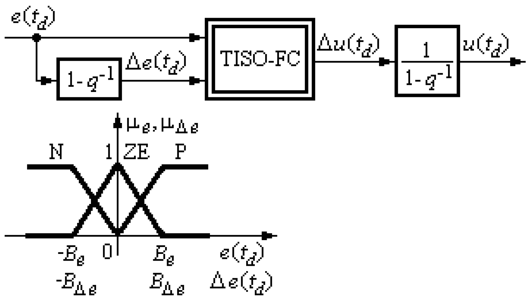
The T-S PI-FCs ensure further performance enhancement by design and tuning starting with the linear PI controllers. The typical structure and input membership functions of a T-S PI-FC are presented in Figure 2, where is the backward shift operator, TISO-FC is the Two Inputs-Single Output fuzzy controller block modeled by a nonlinear input-output static map, is the increment of the control error, and is the increment of the control signal.
These two increments are obtained by discretizing the continuous-time PI controller by Tustin’s method, which leads to the recurrent equation of the incremental discrete-time PI controller and its parameters and [27,28,29]
where is the discrete time index and is the sampling period.
The TISO-FC block in the T-S PI-FC structure uses the weighted average method for defuzzification, and the SUM and PROD operators in the inference engine. The complete rule base of this block consists of the following two rules [21]:
where the parameter , , contributes to the reduction of the control system overshoot.
The application of the modal equivalence principle [30] leads to the tuning equation
and the parameters of the T-S PI-FC are grouped in the parameter vector :
The optimization problems that ensure the sensitivity reduction with respect to the modifications of the process parameter are defined as
where , are the weighting parameters, with the subscript indicating the process parameters indicated in Equation (5), is the optimal parameter vector, i.e., the optimal value of the vector , and is the feasible domain of . The stability of the fuzzy control is recommended to be taken into consideration in order to set the domain , and useful approaches are reported in [23,27,28,29,31,32,33,34,35,36].
The objective function is referred to as the weighted sum of the absolute value of the control error and of the squared output sensitivity function, but the state sensitivity functions can be included as well. Other objective functions can also be considered, inspired from several applications with classical and modern algorithms [37,38,39,40,41,42].
The state sensitivity models of the fuzzy control system with respect to are derived using Equation (6), with for T-S PI-FCs. Accepting that the control signal is changing at the discrete sampling intervals and the zero-order hold is included in the fuzzy control system structure for digital control, the number of four state variables results from the fact that the state variables and of the T-S PI-FC are defined in terms of [7]. The expression of the state sensitivity model of the fuzzy control system with respect to the parameter of the family of nonlinear servo systems is [7]
and the expression of the state sensitivity model of the fuzzy control system with respect to the parameter is [7]
where the state variables of the T-S PI-FC are defined in terms of
is the nonlinear input-output map of TISO-FC, and the dynamics of the reference input filter are not accounted for. The subscript 0 in Equations (14) and (15) outlines the nominal value of the process parameter (as already shown in relation with Equation (6)) and also the nominal trajectory of the fuzzy control system (i.e., the nominal state variables) and the nominal expression of the input-output map of TISO-FC.
3. Grey Wolf Optimizer, Analysis, and Optimal Tuning Approach
This section presents the general description of GWO with the aim of introducing it later into the optimization problems described in the previous section. Based on this information a novel optimal tuning approach is defined in the last part of the section.
3.1. Grey Wolf Optimizer and Analysis
The operating mechanism of GWO according to its standard formulation given in [12] starts with the random initialization of the agents that comprise the wolf pack. A total number of agents (i.e., grey wolves) is used, and each agent is assigned to a position vector
where is the position of agent in the dimension, , is the index of the current iteration, , and is the maximum number of iterations.
The search process specific to GWO continues with the exploration stage, which models the search for the prey. During this stage the positions of the top three agents, namely the alpha (), beta (), and delta () agents, dictate the search pattern by diverging from other agents and converging to the prey, representing the optimal solution.
The exploitation stage models the attack on the prey. The top three agents constrain the other agents (the omega () agents) to update their positions according to theirs. The following notations are used for the top three agent position vectors, i.e., the first three best solutions obtained at each iteration (or the alpha, beta, and delta solutions):
the three vector solutions , , and are obtained by the following selection process:
and they fulfill the condition
A set of search coefficients is then defined:
where and are uniformly distributed random numbers within , , , and the coefficients are linearly decreased from 2 to 0 during the search process:
The approximate distances between the current solution and the alpha, beta, and delta solutions, i.e., , , and , respectively, are
The components (agents) of the updated alpha, beta, and delta solutions are computed as
and they lead to the updated expressions of the agents’ positions obtained as the arithmetic mean of the updated alpha, beta, and delta agents:
The vector counterpart of Equation (25) is the formula that gives the update vector solution :
The GWO consists of the following steps that are formulated by the revision of the steps presented in [20,21]:
Step 1. The initial random grey wolf population, represented by agents’ positions in the -dimensional search space, is generated. The iteration index is initialized to and the maximum number of iterations is set to .
Step 2. The performance of each member of the population of agents is evaluated by simulations and/or experiments conducted on the fuzzy control system. The evaluation leads to the objective function value by mapping the GWO onto the optimization problems using
Step 3. The first three best solutions obtained so far, i.e., , , and , are identified using Equation (19).
Step 4. The search coefficients are calculated using Equations (21) and (22).
Step 5. The agents are moved to their new positions by computing in terms of Equations (24), (25), and (26).
Step 6. The updated vector solution is validated by checking the steady-state condition for the fuzzy control system with the T-S PI-FC parameter vector , so far [7]
where is the final time moment. Theoretically as pointed out in Equation (13), but takes practically a finite value in order to capture the transients in the fuzzy control system responses. The stability analysis of the fuzzy control system can be also employed with this regard.
Step 7. The iteration index is incremented and the algorithm continues with step 2 until is reached.
Step 8. The algorithm is stopped and the final solution obtained so far is actually the solution to the optimization problems defined in Equation (13):
The substitution of taken from Equation (23) in Equation (24) leads to
The computation of the arithmetic mean in Equation (30) for and then the application of Equation (25) at the iterations and are organized as the following state-space equation:
which indicates a nonlinear dynamic system. Such expressions are used in [43,44,45] for other metaheuristics as well (PSO and GSA) and are then associated with stability analyses. However, the nonlinearity in Equation (31) makes the GWO analysis more difficult in comparison with [43,44,45].
Equation (31) is then expressed in the equivalent form
and since the right-hand term in Equation (32) is negative, this indicates that
Using in Equation (22) and then Equation (21), the coefficients obtain the expressions
Using Equation (34) in Equation (32) for , this gives the condition for the final values of the agents’ positions
In addition, Equation (35) used in combination with Equation (33) gives the following condition related to the dynamics of the agents’ positions:
Concluding, Equation (36) indicates that is a monotonic strictly decreasing sequence as this will guarantee the convergence of GWO. Therefore, it is recommended to initialize as large as possible values of .
The stability analysis of the dynamics of the agents’ positions starts with the definition of the Lyapunov function candidate
that fulfils the conditions
The expression of the increment of is
Using Equation (36) in Equation (37), the sufficient condition for the global asymptotic stability of the origin of dynamics of the agents’ positions is
Using taken from Equation (31) in Equation (40), Equation (40) is then transformed into
Since the right-hand term in Equation (41) is strictly positive, Equation (41) leads to the first sufficient condition for the agents’ positions:
which also implies that
Using Equations (42) and (43) and the properties of the modulus, the right-hand term in Equation (41) is upper bounded in terms of
To sum up, in order to fulfill the condition for the global asymptotic stability of the origin of dynamics of the agents’ positions, it is sufficient to fulfill the following condition, as it results from Equations (41) and (44) and the transitive property of inequalities:
which is equivalent to
Since Equation s (21) and (22) lead to
the left-hand term in Equation (46) fulfills the condition
Summing up, the stability analysis should be re-organized in order to check the sufficient stability conditions of Equations (42) and (46) at each iteration. This stability check is recommended to be carried out in step 6 in order to validate the next vector solution by dropping out those agents that do not fulfill the conditions of Equations (42) and (46).
Moreover, Equation (42) indicates that GWO is recommended to solve optimization problems where the variables take positive values. Such problems occur in the optimal tuning of the parameters of several linear and fuzzy controllers or of the positive parameters specific to linear and nonlinear models, including fuzzy ones.
The convergence and stability for negative values of the variables cannot be guaranteed using the above approach. They are guaranteed because of the operating mechanism of GWO, which uses the best three agents at each iteration and drives the solution towards the solution to the optimization problem.
Equations (42) and (46) can be viewed as the basis in the development of adaptive GWO using the knowledge from adaptive PSO, GSA, and CSS [9,23]. One such approach can be supported by replacing the linear decrease of the coefficients in Equation (22) with an exponential one:
Fuzzy logic can be involved in adaptive GWO in order to exploit the advantages of the nonlinear input-output maps of fuzzy systems [46,47,48,49,50]. The hybridization with other algorithms is a good option because of the small numbers of GWO; metaheuristics or classical algorithms can be used with this regard in several applications [51,52,53,54].
3.2. Optimal Tuning Approach
The GWO is mapped onto the optimization problems defined in Equation (13) by the relationships given in Equations (20), (26), and (27). The optimal tuning approach for T-S PI-FC consists of the following steps built around the approach suggested in [21] and the GWO implementation according to the previous sub-section:
Step A. The ESO method is applied to tune the parameters of the linear PI controllers, is set, and the discrete-time PI controllers expressed in Equation (9) are obtained. The particular expressions of the state sensitivity models of the fuzzy control system are derived in accordance with Equations (14) and (15).
Step B. The weighting parameters , specified in Equation (13) are set such that they meet the performance specifications of the fuzzy control system. The parameter is set according to step 6 of GWO, and the domain is set to include all constraints imposed to the elements of .
Step C. GWO implemented according to Sub-Section 3.1 is applied to solve the optimization problems defined in Equation (13), which produce the optimal values of the parameter vector and the optimal parameters , , and :
Step D. The optimal value of the parameter , namely , results from the following particular expression of Equation (11):
Step E. The transfer function of the reference input filter is obtained from the following particular expression of Equation (8):
4. Case Study
Both GWO and the tuning approach are validated in this section by the design and tuning of T-S PI-FCs for the angular position control of an experimental setup [58]. The experimental setup operates in the Intelligent Control Systems Laboratory of the Politehnica University of Timisoara, Romania. The nominal values of the parameters of the process models of Equations (1) and (2) have been obtained by least squares identification algorithms as , , , , and . The simulations were performed using the Matlab environment being run on several machines with various configurations, thus parallelizing the computations in order to reduce the execution time.
The weighting parameters presented in Equation (13) have been defined to satisfy a ratio of of the initial values of the terms presented in the sums. The following values have been used:
The upper limit of the sums in Equation (13) has been set to instead of , which corresponds to the evaluation of the objective functions by experiments conducted on a time horizon of . The vector variables of the objective functions have been initialized and are then validated to belong to the feasible (search) domain
The dynamic regimes characterized by step type modification applied to the reference input and disturbance input have been used. The integral term in the T-S PI-FC structure carries out the disturbance rejection.
The parameters of GWO have been defined based on the designers’ experience and aim to achieve an acceptable balance between convergence and computational resources as and .
The optimal controller parameters and the associated minimum objective function values of the two optimization problems defined in Equation (13) are presented in Table 1 and Table 2.
The quality of GWO is analyzed through three sets of performance indices that try to quantify the use of allocated resources and asses the search process. The first set of performance indexes used in the analysis of the solution quality is the average value of the objective functions and obtained by running several independent runs of GWO and are referred to as and :
where and are the values obtained by running GWO, is the number of best values (i.e., the smallest values) obtained for the objective functions, and the superscript indicates the values of the objective functions obtained by one of the best runs of GWO, namely by the run . The value is considered in the context of the current analysis. The values of this performance index have already been presented in Table 1 and Table 2 for a fair assessment.
For the second set of performance indices, viz. the convergence speed , the number of evaluations of the objective functions until the minimum value is found is looked at. This index is presented as an average value of GWO runs for the first performance index.
The third set of performance indices is introduced with the aim of evaluating the recall of the search process. This set of indices, referred to as the accuracy rate , is defined in terms of the percentage of standard deviation of the objective function value with respect to the average value:
GWO has been compared with the other two metaheuristics to solve the same optimization problems defined in Equation (13). The resulting parameters from [7,9] for the two metaheuristics GSA and PSO that were considered based on their unsupervised characteristics show similar values to the ones already presented.
Another set of experimental results is presented in Table 3 as the values of the performance indices and . These results show that no algorithm has a clear advantage as the values of these sets of performance indices are close. However, GWO is the overall best metaheuristics from the point of view of , and PSO is the overall best one as far as is concerned. The same conclusion has been drawn in [21] for a different optimization problem.
Typical responses for these fuzzy control systems are presented in [21].
5. Conclusions
This paper has proposed an easily understandable optimization algorithm (GWO) applied to the optimal tuning of the parameters of T-S PI-FCs, showing good results in comparison with the other two metaheuristics in the fuzzy control of a family of nonlinear servo systems.
The convergence and stability analysis of GWO indicate that GWO is mainly dedicated to optimization problems where the variables are strictly positive. However, the operating mechanism of GWO based on the use of the best three agents makes it useful in other optimization problems as well without guaranteeing the convergence.
GWO is advantageous over other metaheuristics because of the reduced number of random parameters and user-selected parameters. This illustrates its potential in solving various optimization problems with a reduced user experience and fair comparison with similar metaheuristics.
The performance obtained by GWO is encouraging and comparable to PSO and GSA. Future research will be focused on the performance improvement of GWO by its inclusion in adaptive and hybrid optimization algorithms.
Acknowledgments
This work was supported by grants from the Partnerships in priority areas—PN II program of the Romanian Ministry of Research and Innovation—the Executive Agency for Higher Education, Research, Development and Innovation Funding (UEFISCDI), project numbers PN-II-PT-PCCA-2013-4-0544 and PN-II-PT-PCCA-2013-4-0070, by a grant from the Romanian National Authority for Scientific Research (CNCS)–UEFISCDI, project number PN-II-RU-TE-2014-4-0207, and by a grant from the NSERC of Canada.
Author Contributions
Radu-Emil Precup wrote the paper and analyzed the algorithms; Radu-Codrut David implemented the algorithms and the controllers, performed the simulations, and revised the paper; Alexandra-Iulia Szedlak-Stinean conceived and designed the experiments, performed the experiments, and revised the paper; Emil M. Petriu wrote and revised the paper; Florin Dragan ensured the hardware and software support. All authors have read and approved the final paper.
Conflicts of Interest
The authors declare no conflict of interest.
References
- Castillo, O.; Martinez-Marroquin, R.; Melin, P.; Valdez, F.; Soria, J. Comparative study of bio-inspired algorithms applied to the optimization of type-1 and type-2 fuzzy controllers for an autonomous mobile robot. Inf. Sci. 2012, 192, 19–38. [Google Scholar]
- Castillo, O.; Melin, P. A review on interval type-2 fuzzy logic applications in intelligent control. Inf. Sci. 2014, 279, 615–631. [Google Scholar] [CrossRef]
- Precup, R.-E.; Angelov, P.; Costa, B.S.J.; Sayed-Mouchaweh, M. An overview on fault diagnosis and nature-inspired optimal control of industrial process applications. Comput. Ind. 2015, 74, 75–94. [Google Scholar] [CrossRef]
- Bouallègue, S.; Haggège, J.; Ayadi, M.; Benrejeb, M. PID-type fuzzy logic controller tuning based on particle swarm optimization. Eng. Appl. Artif. Intell. 2012, 25, 484–493. [Google Scholar] [CrossRef]
- Tran, H.-K.; Chiou, J.-S. PSO-based algorithm applied to quadcopter micro air vehicle controller design. Micromachines 2016, 7, 168. [Google Scholar]
- Sahu, R.K.; Panda, S.; Chandra Sekhar, G.T. A novel hybrid PSO-PS optimized fuzzy PI controller for AGC in multi area interconnected power systems. Int. J. Electr. Power Energy Syst. 2015, 64, 880–893. [Google Scholar]
- David, R.-C.; Precup, R.-E.; Petriu, E.M.; Radac, M.-B.; Preitl, S. Gravitational search algorithm-based design of fuzzy control systems with a reduced parametric sensitivity. Inf. Sci. 2013, 247, 154–173. [Google Scholar] [CrossRef]
- Azadani, H.N.; Torkzadeh, R. Design of GA optimized fuzzy logic-based PID controller for the two area non-reheat thermal power system. In Proceedings of the 13th Iranian Conference on Fuzzy Systems, Qazvin, Iran, 27–29 August 2013; pp. 1–6. [Google Scholar]
- Precup, R.-E.; David, R.-C.; Petriu, E.M.; Preitl, S.; Radac, M.-B. Novel adaptive charged system search algorithm for optimal tuning of fuzzy controllers. Expert Syst. Appl. 2014, 41, 1168–1175. [Google Scholar]
- Castillo, O.; Neyoy, H.; Soria, J.; Melin, P.; Valdez, F. A new approach for dynamic fuzzy logic parameter tuning in ant colony optimization and its application in fuzzy control of a mobile robot. Appl. Soft Comput. 2015, 28, 150–159. [Google Scholar] [CrossRef]
- Castillo, O.; Lizárraga, E.; Soria, J.; Melin, P.; Valdez, F. New approach using ant colony optimization with ant set partition for fuzzy control design applied to the ball and beam system. Inf. Sci. 2015, 294, 203–215. [Google Scholar] [CrossRef]
- Mirjalili, S.; Mirjalili, S.M.; Lewis, A. Grey wolf optimizer. Adv. Eng. Softw. 2014, 69, 46–61. [Google Scholar] [CrossRef]
- Mahdad, B.; Srairi, K. Blackout risk prevention in a smart grid based flexible optimal strategy using grey wolf-pattern search algorithms. Energy Convers. Manag. 2015, 98, 411–429. [Google Scholar] [CrossRef]
- Mirjalili, S. How effective is the grey wolf optimizer in training multi-layer perceptrons. Appl. Intell. 2015, 43, 150–161. [Google Scholar] [CrossRef]
- Sulaiman, M.H.; Mustaffa, Z.; Mohamed, M.R.; Aliman, O. Using the grey wolf optimizer for solving optimal reactive power dispatch problem. Appl. Soft Comput. 2015, 32, 286–292. [Google Scholar] [CrossRef]
- Saremi, S.; Mirjalili, S.Z.; Mirjalili, S.M. Evolutionary population dynamics and grey wolf optimizer. Neural Comput. Appl. 2015, 26, 1257–1263. [Google Scholar] [CrossRef]
- Medjahed, S.A.; Saadi, T.A.; Benyettou, A.; Ouali, M. Gray wolf optimizer for hyperspectral band selection. Appl. Soft Comput. 2016, 40, 178–186. [Google Scholar] [CrossRef]
- Yang, B.; Zhang, X.-S.; Yu, T.; Shu, H.-C.; Fang, Z.-H. Grouped grey wolf optimizer for maximum power point tracking of doubly-fed induction generator based wind turbine. Energy Convers. Manag. 2017, 133, 427–443. [Google Scholar] [CrossRef]
- Noshadi, A.; Shi, J.; Lee, W.S.; Shi, P.; Kalam, A. Optimal PID-type fuzzy logic controller for a multi-input multi-output active magnetic bearing system. Neural Comput. Appl. 2016, 27, 2031–2046. [Google Scholar] [CrossRef]
- Precup, R.-E.; David, R.-C.; Petriu, E.M.; Szedlak-Stinean, A.-I.; Bojan-Dragos, C.-A. Grey wolf optimizer-based approach to the tuning of PI-fuzzy controllers with a reduced process parametric sensitivity. IFAC-Pap. Online 2016, 48, 55–60. [Google Scholar] [CrossRef]
- Precup, R.-E.; David, R.-C.; Petriu, E.M. Grey wolf optimizer algorithm-based tuning of fuzzy control systems with reduced parametric sensitivity. IEEE Trans. Ind. Electron. 2017, 64, 527–534. [Google Scholar] [CrossRef]
- Precup, R.-E.; David, R.-C.; Petriu, E.M.; Preitl, S.; Radac, M.-B. Gravitational search algorithms in fuzzy control systems tuning. In Proceedings of the 18th IFAC World Congress, Milano, Italy, 28 August–2 September 2011; pp. 13624–13629. [Google Scholar]
- Precup, R.-E.; David, R.-C.; Petriu, E.M.; Radac, M.-B.; Preitl, S. Adaptive GSA-based optimal tuning of PI controlled servo systems with reduced process parametric sensitivity, robust stability and controller robustness. IEEE Trans. Cybern. 2014, 44, 1997–2009. [Google Scholar] [CrossRef] [PubMed]
- Precup, R.-E.; Sabau, M.-C.; Petriu, E.M. Nature-inspired optimal tuning of input membership functions of Takagi-Sugeno-Kang fuzzy models for anti-lock braking systems. Appl. Soft Comput. 2015, 27, 575–589. [Google Scholar] [CrossRef]
- Preitl, S.; Precup, R.-E. On the algorithmic design of a class of control systems based on providing the symmetry of open-loop Bode plots. Sci. Bull. UPT Trans. Autom. Control Comput. Sci. 1996, 41, 47–55. [Google Scholar]
- Preitl, S.; Precup, R.-E. An extension of tuning relations after symmetrical optimum method for PI and PID controllers. Automatica 1999, 35, 1731–1736. [Google Scholar] [CrossRef]
- Precup, R.-E.; Doboli, S.; Preitl, S. Stability analysis and development of a class of fuzzy control systems. Eng. Appl. Artif. Intell. 2000, 13, 237–247. [Google Scholar] [CrossRef]
- Precup, R.-E.; Preitl, S. PI-fuzzy controllers for integral plants to ensure robust stability. Inf. Sci. 2007, 177, 4410–4429. [Google Scholar] [CrossRef]
- Precup, R.-E.; Radac, M.-B.; Tomescu, M.L.; Petriu, E.M.; Preitl, S. Stable and convergent iterative feedback tuning of fuzzy controllers for discrete-time SISO systems. Expert Syst. Appl. 2013, 40, 188–199. [Google Scholar] [CrossRef]
- Galichet, S.; Foulloy, L. Fuzzy controllers: Synthesis and equivalences. IEEE Trans. Fuzzy Syst. 1995, 3, 140–148. [Google Scholar] [CrossRef]
- Precup, R.-E.; Preitl, S. Popov-type stability analysis method for fuzzy control systems. In Proceedings of the Fifth European Congress on Intelligent Technologies and Soft Computing, Aachen, Germany, 8–11 September 1997; Volume 2, pp. 1306–1310. [Google Scholar]
- Kluska, J. Absolute stability of continuous fuzzy control systems. In Stability Issues in Fuzzy Control; Aracil, J., Gordillo, F., Eds.; Springer-Verlag: Berlin/Heidelberg, Germany; New York, NY, USA, 2000; Studies in Fuzziness and Soft Computing; Volume 44, pp. 15–45. [Google Scholar]
- Baranyi, P.; Tikk, D.; Yam, Y.; Patton, R.J. From differential equations to PDC controller design via numerical transformation. Comput. Ind. 2003, 51, 281–297. [Google Scholar] [CrossRef]
- Škrjanc, I.; Blažič, S. Predictive functional control based on fuzzy model: Design and stability study. J. Intell. Robot. Syst. 2005, 43, 283–299. [Google Scholar] [CrossRef]
- Driss, Z.; Mansouri, N. A novel adaptive approach for synchronization of uncertain chaotic systems using fuzzy PI controller and active control method. Control Eng. Appl. Inform. 2016, 18, 3–13. [Google Scholar]
- Liu, C.; Lam, H.-K.; Ban, X.-J.; Zhao, X.-D. Design of polynomial fuzzy observer-controller with membership functions using unmeasurable premise variables for nonlinear systems. Inf. Sci. 2016, 355–356, 186–207. [Google Scholar] [CrossRef]
- Delprat, S.; Lauber, J.; Guerra, T.-M.; Rimaux, J. Control of a parallel hybrid powertrain: Optimal control. IEEE Trans. Veh. Technol. 2004, 53, 872–881. [Google Scholar] [CrossRef]
- Filip, F.G. Decision support and control for large-scale complex systems. Ann. Rev. Control 2008, 32, 61–70. [Google Scholar] [CrossRef]
- Qin, Q.-D.; Cheng, S.; Zhang, Q.-Y.; Li, L.; Shi, Y.-H. Biomimicry of parasitic behavior in a coevolutionary particle swarm optimization algorithm for global optimization. Appl. Soft Comput. 2015, 32, 224–240. [Google Scholar] [CrossRef]
- Ghosn, S.B.; Drouby, F.; Harmanani, H.M. A parallel genetic algorithm for the open-shop scheduling problem using deterministic and random moves. Int. J. Artif. Intell. 2016, 14, 130–144. [Google Scholar]
- Osaba, E.; Yang, X.-S.; Diaz, F.; Lopez, P.; Carballedo, R. An improved discrete bat algorithm for symmetric and asymmetric traveling salesman problems. Eng. Appl. Artif. Intell. 2016, 48, 59–71. [Google Scholar] [CrossRef]
- Azar, D.; Fayad, K.; Daoud, C. A combined ant colony optimization and simulated annealing algorithm to assess stability and fault-proneness of classes based on internal software quality attributes. Int. J. Artif. Intell. 2016, 14, 137–156. [Google Scholar]
- Kadirkamanathan, V.; Selvarajah, K.; Fleming, P.J. Stability analysis of the particle dynamics in particle swarm optimizer. IEEE Trans. Evol. Comput. 2006, 10, 245–253. [Google Scholar] [CrossRef]
- Jiang, S.-H.; Wang, Y.; Jia, Z.-C. Convergence analysis and performance of an improved gravitational search algorithm. Appl. Soft Comput. 2014, 24, 363–384. [Google Scholar] [CrossRef]
- Farivar, F.; Shoorehdeli, M.A. Stability analysis of particle dynamics in gravitational search optimization algorithm. Inf. Sci. 2016, 337–338, 25–43. [Google Scholar] [CrossRef]
- Gajate, A.; Haber, R.E.; Vega, P.I.; Alique, J.R. A transductive neuro-fuzzy controller: Application to a drilling process. IEEE Trans. Neural Netw. 2010, 21, 1158–1167. [Google Scholar] [CrossRef] [PubMed]
- Angelov, P.; Yager, R. A new type of simplified fuzzy rule-based systems. Int. J. Gen. Syst. 2012, 41, 163–185. [Google Scholar] [CrossRef]
- Chen, T.; Liao, T.W.; Yu, F.-S. Fuzzy collaborative intelligence and systems. Int. J. Intell. Syst. 2015, 30, 617–619. [Google Scholar] [CrossRef]
- Teodorescu, H.-N.L. Revisiting models of vulnerabilities of the networks. Stud. Inform. Control 2016, 25, 469–478. [Google Scholar] [CrossRef]
- Li, H.-Y.; Yeh, R.-G.; Lin, Y.-C.; Lin, L.-Y.; Zhao, J.; Lin, C.-M.; Rudas, I.J. Medical sample classifier design using fuzzy cerebellar model neural networks. Acta Polytech. Hung. 2016, 13, 7–24. [Google Scholar]
- Formentin, S.; Karimi, A.; Savaresi, S.M. Optimal input design for direct data-driven tuning of model-reference controllers. Automatica 2013, 49, 1874–1882. [Google Scholar] [CrossRef]
- Chiarandini, M.; Kjeldsen, N.H.; Nepomuceno, N. Integrated planning of biomass inventory and energy production. IEEE Trans. Comput. 2014, 63, 102–114. [Google Scholar] [CrossRef]
- Molnár, S.; Szidarovszky, F. An alternative method in optimizing random outcomes. Acta Polytech. Hung. 2016, 13, 77–86. [Google Scholar]
- Salcedo-Sanz, S.; García-Díaz, P.; Del Ser, J.; Bilbao, M.N.; Portilla-Figueras, J.A. A novel grouping coral reefs optimization algorithm for optimal mobile network deployment problems under electromagnetic pollution and capacity control criteria. Expert Syst. Appl. 2016, 55, 388–402. [Google Scholar] [CrossRef]
- Navarro, G.; Manic, M. FuSnap: Fuzzy control of logical volume snapshot replication for disk arrays. IEEE Trans. Ind. Electron. 2011, 58, 4436–4444. [Google Scholar] [CrossRef]
- Hanchevici, A.-B.; Patrascu, M.; Dumitrache, I. A hybrid PID-fuzzy control for linear SISO systems with variant communication delays. Adv. Fuzzy Syst. 2012, 2012, 217068:1–217068:8. [Google Scholar] [CrossRef]
- Jahandari, S.; Kalhor, A.; Araabi, B.N. A self tuning regulator design for nonlinear time varying systems based on evolving linear models. Evol. Syst. 2016, 7, 159–172. [Google Scholar] [CrossRef]
- Inteco Ltd. Modular Servo System, User’s Manual; Inteco Ltd.: Krakow, Poland, 2007. [Google Scholar]
Figure 1.
Structure of the fuzzy control system, .
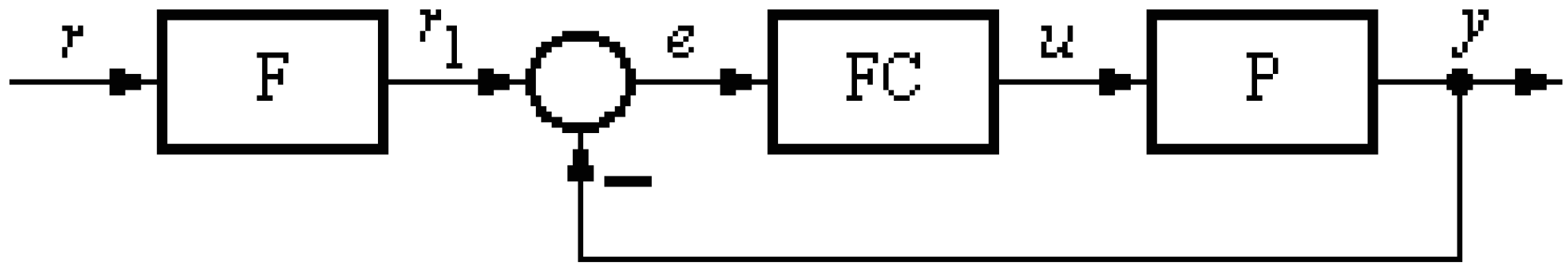
Figure 2.
Structure and input membership functions of the Takagi-Sugeno proportional-integral-fuzzy controller.
Figure 2.
Structure and input membership functions of the Takagi-Sugeno proportional-integral-fuzzy controller.


Table 1.
Weighting parameter and controller parameters for the minimization of .
| 0.006858 | 0.085588 | 40 | 0.747404 | 5.08539 | 0.003443 | 4.67856 | 32604.4 |
| 0.06858 | 0.085016 | 40 | 0.740636 | 5.11954 | 0.003431 | 4.70998 | 118689 |
| 0.6858 | 0.012792 | 20 | 0.250669 | 17 | 0.001883 | 15.64 | 873561 |
Table 2.
Weighting parameter and controller parameters for the minimization of .
| 0.0066695 | 0.0855753 | 40 | 0.75 | 5.08614 | 0.00344263 | 4.67925 | 32497.9 |
| 0.066695 | 0.0844424 | 40 | 0.736102 | 5.1543 | 0.00341979 | 4.74196 | 109271 |
| 0.66695 | 0.0127918 | 20 | 0.250173 | 17 | 0.00188304 | 15.64 | 864912 |
Table 3.
Average values of and .
| for GWO | for GWO | for PSO | for PSO | for GSA | for GSA | |
| 0.006858 | 1865 | 0.9279 | 1933 | 0.0077 | 2322 | 0.8329 |
| 0.06858 | 1237 | 0.1327 | 1185 | 0.0011 | 1477 | 0.1191 |
| 0.6858 | 1461 | 0.2946 | 1559 | 0.0070 | 1685 | 0.1334 |
| for GWO | for GWO | for PSO | for PSO | for GSA | for GSA | |
| 0.0066695 | 1313 | 0.8496 | 2169 | 0.0071 | 1634 | 0.7626 |
| 0.066695 | 965 | 0.1254 | 1080 | 0.1326 | 990 | 0.1745 |
| 0.66695 | 1529 | 0.2387 | 1578 | 0.0057 | 1997 | 0.1080 |
© 2017 by the authors. Licensee MDPI, Basel, Switzerland. This article is an open access article distributed under the terms and conditions of the Creative Commons Attribution (CC BY) license (http://creativecommons.org/licenses/by/4.0/).
Share and Cite
MDPI and ACS Style
Precup, R.-E.; David, R.-C.; Szedlak-Stinean, A.-I.; Petriu, E.M.; Dragan, F. An Easily Understandable Grey Wolf Optimizer and Its Application to Fuzzy Controller Tuning. Algorithms 2017, 10, 68. https://doi.org/10.3390/a10020068
AMA Style
Precup R-E, David R-C, Szedlak-Stinean A-I, Petriu EM, Dragan F. An Easily Understandable Grey Wolf Optimizer and Its Application to Fuzzy Controller Tuning. Algorithms. 2017; 10(2):68. https://doi.org/10.3390/a10020068
Chicago/Turabian StylePrecup, Radu-Emil, Radu-Codrut David, Alexandra-Iulia Szedlak-Stinean, Emil M. Petriu, and Florin Dragan. 2017. "An Easily Understandable Grey Wolf Optimizer and Its Application to Fuzzy Controller Tuning" Algorithms 10, no. 2: 68. https://doi.org/10.3390/a10020068
Note that from the first issue of 2016, this journal uses article numbers instead of page numbers. See further details here.