
Application of Gradient Descent Continuous Actor-Critic Algorithm for Bilateral Spot Electricity Market Modeling Considering Renewable Power Penetration


Abstract
:1. Introduction
2. Multi-Agent Hour-Ahead EM Modeling
- (1)
- Every GenCO (NRGenCO and RPGenCO) has only one generation unit;
- (2)
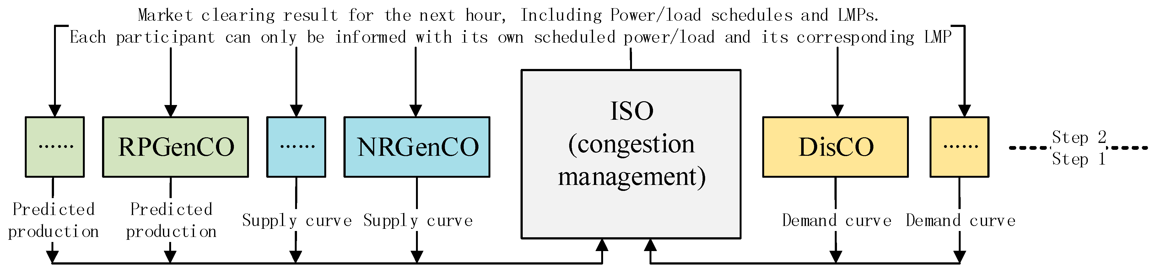
- Similar to [2], the considered hour-ahead EM is a single period EM, hence each hour every NRGenCO and DisCO sends its bid curve for the next hour to the ISO. However, the proposed single-period EM modeling approach can be extended to a multi-period one such as a day-ahead EM;
- (3)
- Each hour, every RPGenCO submits only its own predicted production with bidding price 0 ($/MW) for the next hour to ISO because of its low marginal cost and the role of “price taker” [2,33,35], and the only strategic players are NRGenCOs [2] and DisCOs. Therefore, each NRGenCO and DisCO can be considered an agent that adaptively adjusts the bidding strategy in order to maximize profit.
3. Definitions
- (1)
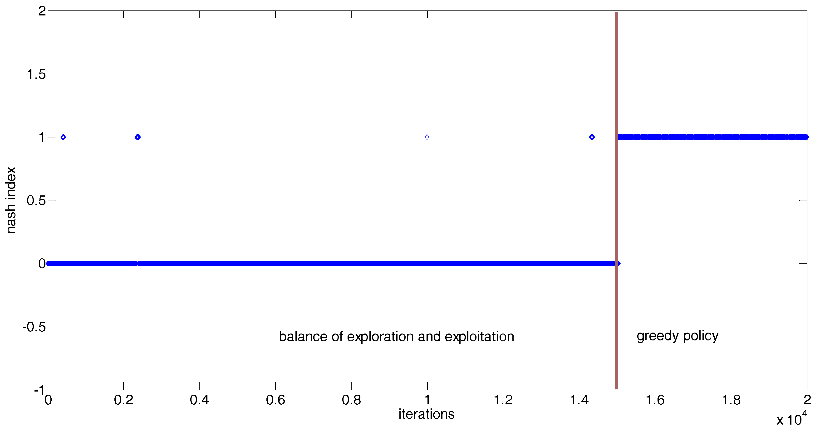
- Iteration: since the market is assumed to be cleared on an hour-ahead basis, we consider each hour as an iteration [2]. Moreover, just like in [2], time differences between hours such as demand preference, generation ramping constraints, number of participants, etc. are neglected. The purpose of doing this is to test whether the proposed modeling approach can automatically converge to the Nash equilibrium (NE) or not under the condition of no other external interference.
- (2)
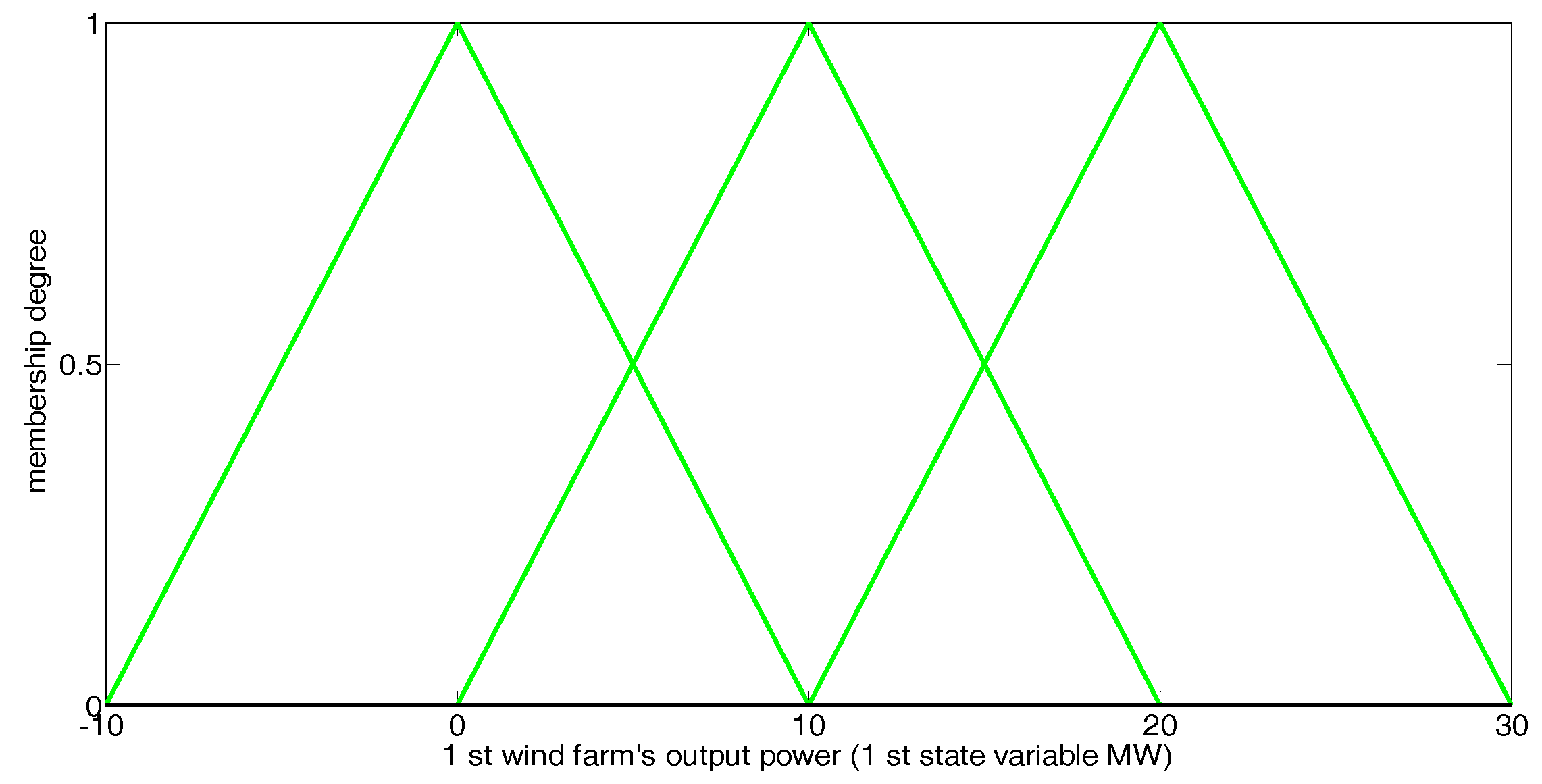
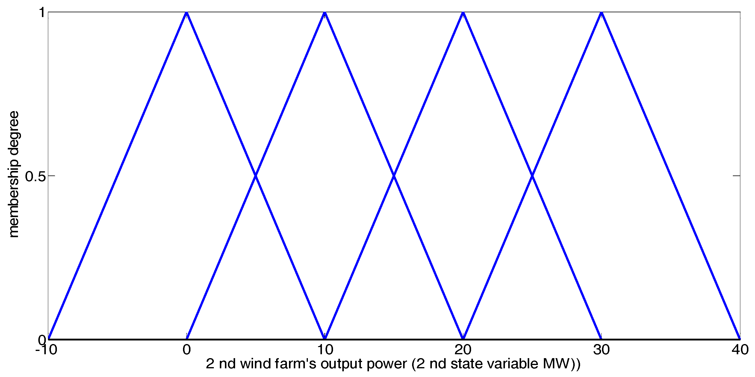
- State variable: in iteration t, the predicted power production of each RPGenCO can be defined as one state variable of the EM environment [2]. Due to the intermittent and random nature of the renewable power production, the vth state variable, representing the predicted power production of RPGenCO v, is a random variable, and can be represent as:where randomly changes within a continuous interval of scalar values over time [2]:Hence, in iteration t, all state variables together constitute a state vector:where represents the continuous state space of the EM environment.
- (3)
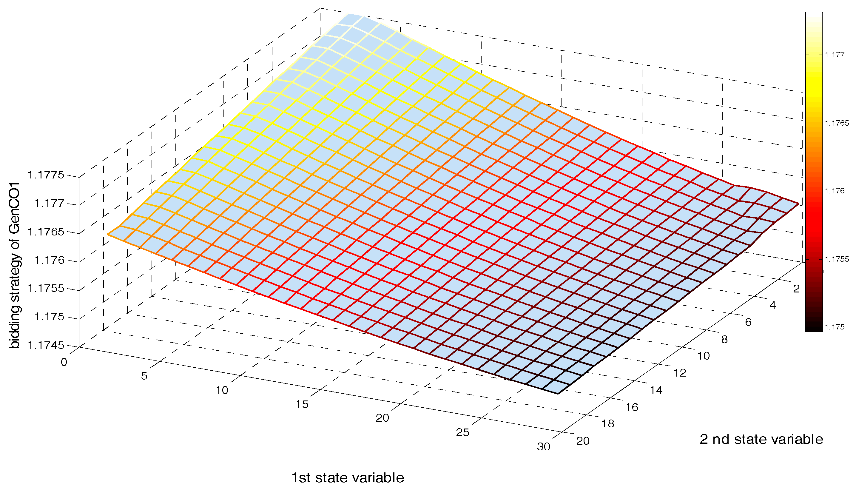
- Action variable: the bidding strategy of every NRGenCO and DisCO is defined as one action variable of an agent. The ith action variable, representing the bidding strategy of NRGenCO i, in iteration t is:The jth action variable, representing the bidding strategy of DisCO j, in iteration t is:All s and s can be adjusted, by the corresponding agent, within continuous intervals of scalar values over time, because an agent may not be able to achieve its maximum profit when selecting bidding strategies within a discrete action set.
- (4)
- Reward: In iteration t, NRGenCO i’s (i = 1, 2, …,Ng1) reward is:DisCO j’s (j = 1, 2, …, Nd ) reward in iteration t is:where () is the LMP of the bus connecting NRGenCOi (DisCOj), and () is the cost (revenue) of NRGenCO i (DisCO j) when its dispatched power production (power demand) is ().
4. Applying the GDCAC Algorithm for EM Modeling Considering Renewable Power Penetration
4.1. Introduction of Gradient Descent Continuous Actor-Critic Algorithm
4.2. The Proposed GDCAC-Based EM Procedure Considering Renewable Power Penetration
- (1)
- Input: for NRGenCOi () : , step length parameter series and ; for DisCOj () : , step length parameter series and ; and parameters for every NRGenCO and DisCO.
- (2)
- T = 1.
- (3)
- Initialize the linear parameter vectors and for NRGenCOi (), linear parameter vectors and for DisCOj ().
- (4)
- Random state generation: in iteration t, a random point, , is generated in the continuous state space , which represents the continuous state space of power productions by all RPGenCOs.
- (5)
- In iteration t, NRGenCOi () chooses and implements an action () from state xt, DisCOj () chooses and implements an action () from state xt, and then ISO implements the congestion management model considering renewable power penetration represented by Equations (5)–(11).
- (6)
- NRGenCOi () observes the immediate reword rgi,t using Equation (19) and DisCOj () observes the immediate reward rdj,t using Equation (20).
- (7)
- Discount factor setting: because is a stochastic variable independent from () and (), every NRGenCO and DisCO has no idea what the true value of while in iteration t. Therefore, similar to [2], we assume that the discount factor for every NRGenCO and DisCO in iteration t equals 0.
- (8)
- Learning: in this step, and for NRGenCOi () as well as and for DisCOj () are updated using TD(0) error and the gradient descent method:NRGenCOi:DisCO j:
- (9)
- T = t + 1.
- (10)
- If , return to (4). T is the terminal number of iterations.
- (11)
- Output: for NRGenCO i: and Vgi*(x), Agi*(x); for GenCO i: and Vdj*(x), Adj*(x).
5. Discussion of Simulations and Results
5.1. Data and Assumptions
5.2. Implementing a GDCAC-Based Approach on the Test System
5.3. Comparative Study
- (1)
- No matter which of the three sample states, in Table 5, NRGenCO1’s final profit in Scenario 1 is 369.5193 ($/h), which is more than that in Scenario 2 (296.7915 ($/h)). In Table 6, NRGenCO1’s final profit in Scenario 1 is 484.2735 ($/h), which is more than that in Scenario 2 (408.0777 ($/h)). In Table 7, NRGenCO1’s final profit in Scenario 1 is 326.8942 ($/h), which is more than that in Scenario 2 (304.4191 ($/h)). Moreover, although we cannot compare NRGenCO1’s final profits in Scenarios 1 and 2 under every state point due to the continuous state space, the phenomenon that NRGenCO1’s final profit in Scenario 1 is more than its final profit in Scenario 2 can actually be found under every state point of the sample states in . As mentioned in Section 5.1, there is only one difference between Scenarios 1 and 2, which is that NRGenCO1 in Scenario 1 is a GDCAC-based agent that makes its bidding decisions based on our proposed GDCAC approach, while NRGenCO1 in Scenario 2 is a fuzzy Q-learning-based agent that makes its bidding decisions based on the fuzzy Q-learning approach. Therefore, it can, to some extent, be verified that a specific participant can get more profit with our proposed GDCAC approach in market competition than with the fuzzy Q-learning one proposed in [2].
- (2)
- No matter which of the three sample states, in Table 5, the order of final SWs in the three scenarios from high to low is Scenario 1 (6177.1 ($/h)), Scenario 2 (6108.2 ($/h)), and Scenario 3 (6063.4 ($/h)). In Table 6, the order of final SWs in the three scenarios from high to low is: Scenario 1 (5172.2 ($/h)), Scenario 2 (5123.6 ($/h)), and Scenario 3 (5102.5 ($/h)). In Table 7, the order of the final SWs in the three scenarios from high to low is: Scenario 1 (4639.1 ($/h)), Scenario 2 (4610.7 ($/h)), and Scenario 3 (4562.7 ($/h)). Moreover, although we cannot compare final SWs in Scenarios 1, 2 and 3 for every state point due to the continuous state space, the phenomenon that the order of the final SWs in the three scenarios from high to low are Scenario 1, Scenario 2, and Scenario 3 can actually be found under every state point of the sample states in . As mentioned in Section 5.1, every participant in Scenario 3 is a fuzzy Q-learning-based agent; NRGenCO1 in Scenario 2 is a fuzzy Q-learning-based agent while all the other participants in Scenario 2 are our proposed GDCAC-based ones, and every participant in Scenario 1 is our proposed GDCAC-based agent. Therefore, it can, to some extent, be verified that with the increase in the number of participants applying our proposed approach as their bidding decision-making tool, SW in the market increases.
- (1)
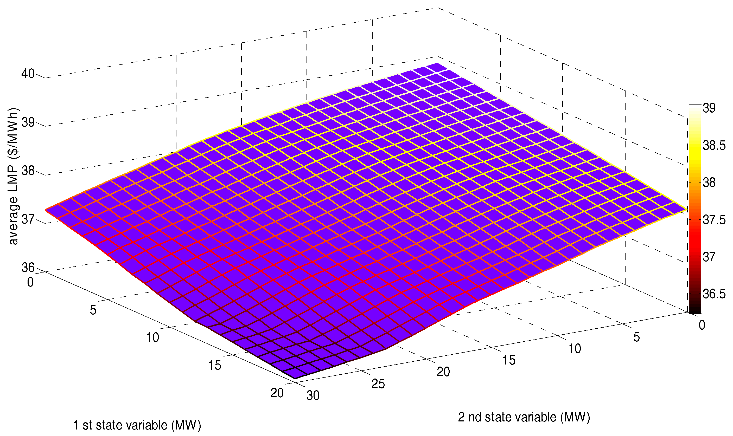
- The order of final average AVLMPs of sample states in the three scenarios, from low to high, is: Scenario 1 (37.0352 ($/MWh)), Scenario 2 (37.4531 ($/MWh)), and Scenario 3 (38.2237 ($/MWh)), which, to some extent, verifies the renewable power penetration in EM. The final average AVLMP of the sample states will be lowered by increasing the number of GDCAC-based agents.
- (2)
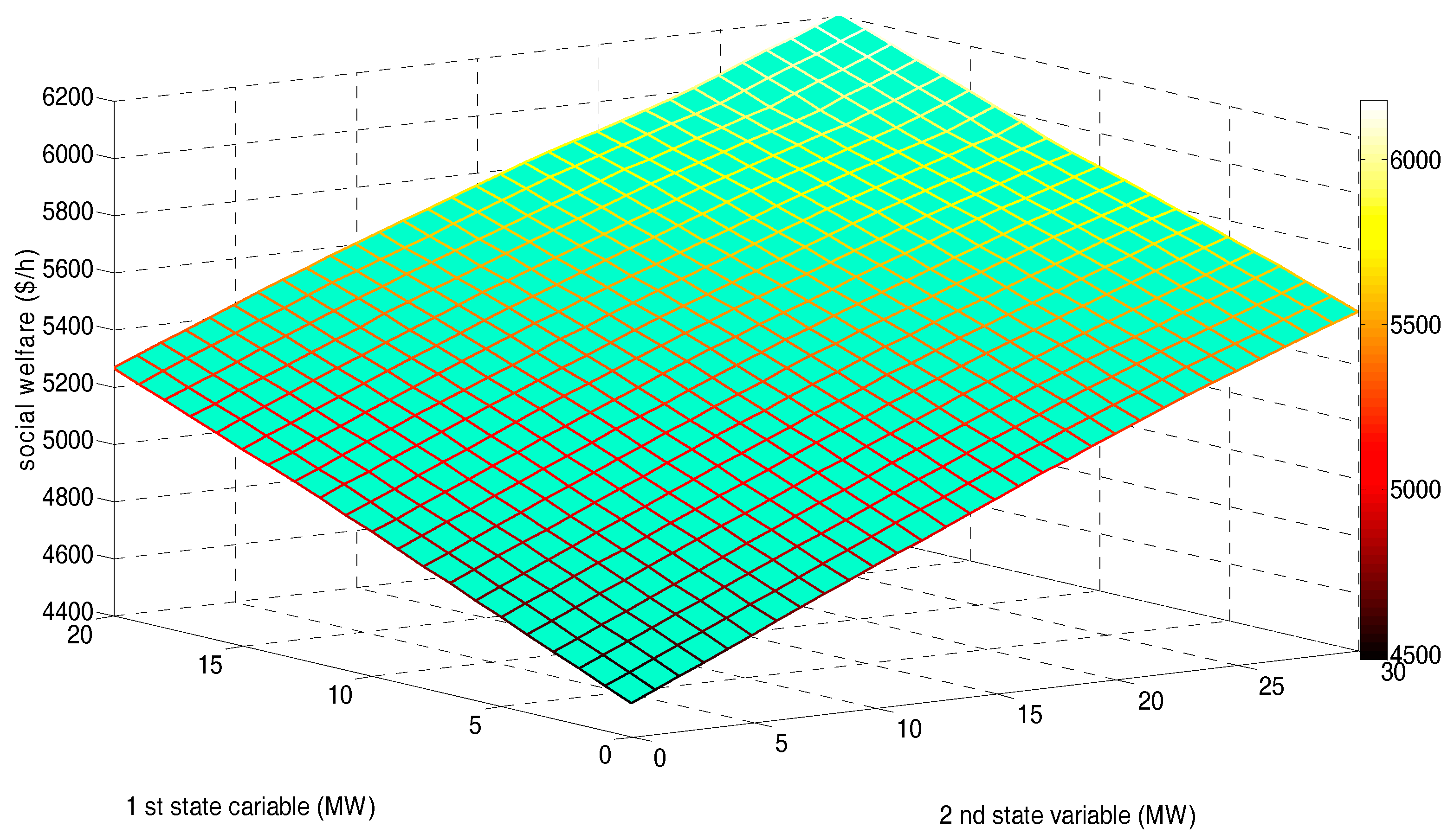
- The order of final average SWs of sample states in the three scenarios from high to low is: Scenario 1 (5329.5 ($/h)), Scenario 2 (5280.8 ($/h)), and Scenario 3 (5242.9 ($/h)), which, to some extent, verifies the renewable power penetration in EM. The final average SW of sample states will be increased by increasing the number of GDCAC-based agents.
- (3)
- Increasing SW as well as lowering clearing prices (represented by average AVLMPs) stands for the economic efficiency improvement in the whole market, which is proven, to some extent and through this comparative study, to be attributable to our proposed GDCAC approach.
6. Conclusions
- (1)
- In our proposed GDCAC-based EM modeling approach, every agent needs no common knowledge about other agents’ costs or revenue functions, etc. and can make the decision to select an optimal bidding strategy within a continuous interval of values according to many renewable power generations randomly changing within a continuous state space, which can avoid the “Curse of Dimensionality”. The randomly fluctuating nature of renewable resource output does not affect the proposed EM approach’s ability to reach NE after enough iterations;
- (2)
- In our proposed GDCAC EM modeling approach, after enough iterations, although with the increase of renewable resource output some agents may have their bidding functions deviate more from their actual marginal cost or revenue functions because of congestions in some transmission lines, the overall SW still increases, which is the same as the conclusions drawn in [2];
- (3)
- Our proposed GDCAC EM modeling approach is superior to the fuzzy Q-learning approach (mentioned in [2]) in terms of increasing the profit of a specific agent and the overall SW and lowering the overall LMP level;
- (4)
- According to [40], the time complexity of GDCAC is O(n) (the relevant mathematical proof is proposed in [40]). However, when applying the GDCAC algorithm to EM modeling, because in every iteration we use the active set (AS) algorithm to solve the congestion management model for ISO, which needs 500 extra iterations, the time complexity of our proposed GDCAC-based EM modeling approach is O(500n). Nevertheless, our simulation with the proposed GDCAC-based EM modeling approach takes only about 3.2 min to reach the final result. That is to say, the time complexity of our GDCAC-based EM modeling approach is acceptable so that we can extend it to the modeling and simulation of more realistic and complex EM systems.
Acknowledgments
Author Contributions
Conflicts of Interest
References
- Alikhanzadeh, A.; Irving, M. Combined oligopoly and oligopsony bilateral electricity market model using CV equilibria. In Proceedings of the 2012 IEEE Power and Energy Society General Meeting, San Diego, CA, USA, 22–26 July 2012; pp. 1–8. [Google Scholar]
- Mohammad, R.S.; Salman, S. Application of fuzzy Q-learning for electricity market modeling by considering renewable power penetration. Renew. Sustain. Energy Rev. 2016, 56, 1172–1181. [Google Scholar]
- Aghaei, J.; Akbari, M.; Roosta, A.; Gitizadeh, M.; Niknam, T. Integrated renewable-conventional generation expansion planning using multi objective framework. IET Gener. Transm. Distrib. 2012, 6, 773–784. [Google Scholar] [CrossRef]
- Yu, N.; Liu, C.C.; Tesfatsion, L. Modeling of Suppliers' Learning Behaviors in an Electricity Market Environment. In Proceedings of the 2007 International Conference on Intelligent Systems, Niigata, Japan, 5–8 November 2007; pp. 1–6. [Google Scholar]
- Widén, J.; Carpman, N.; Castellucci, V.; Lingfors, D.; Olauson, J.; Remouit, F.; Bergkvist, M.; Grabbe, M.; Waters, R. Variability assessment and forecasting of renewables: A review for solar, wind, wave and tidal resources. Renew. Sustain. Energy Rev. 2015, 44, 356–375. [Google Scholar] [CrossRef]
- Buygi, M.O.; Zareipour, H.; Rosehart, W.D. Impacts of Large-Scale Integration of Intermittent Resources on Electricity Markets: A Supply Function Equilibrium Approach. IEEE Syst. J. 2012, 6, 220–232. [Google Scholar] [CrossRef]
- Al-Agtash, S.Y. Supply curve bidding of electricity in constrained power networks. Energy 2010, 35, 2886–2892. [Google Scholar] [CrossRef]
- Gao, F.; Sheble, G.B.; Hedman, K.W.; Yu, C.-N. Optimal bidding strategy for GENCOs based on parametric linear programming considering incomplete information. Int. J. Electr. Power Energy Syst. 2015, 66, 272–279. [Google Scholar] [CrossRef]
- Borghetti, A.; Massucco, S.; Silvestro, F. Influence of feasibility constrains on the bidding strategy selection in a day-ahead electricity market session. Electr. Power Syst. Res. 2009, 79, 1727–1737. [Google Scholar] [CrossRef]
- Kumar, J.V.; Kumar, D.M.V. Generation bidding strategy in a pool based electricity market using Shuffled Frog Leaping Algorithm. Appl. Soft Comput. 2014, 21, 407–414. [Google Scholar] [CrossRef]
- Wang, J.; Zhou, Z.; Botterud, A. An evolutionary game approach to analyzing bidding strategies in electricity markets with elastic demand. Energy 2011, 36, 3459–3467. [Google Scholar] [CrossRef]
- Min, C.G.; Kim, M.K.; Park, J.K.; Yoon, Y.T. Game-theory-based generation maintenance scheduling in electricity markets. Energy 2013, 55, 310–318. [Google Scholar] [CrossRef]
- Shivaie, M.; Ameli, M.T. An environmental/techno-economic approach for bidding strategy in security-constrained electricity markets by a bi-level harmony search algorithm. Renew. Energy 2015, 83, 881–896. [Google Scholar] [CrossRef]
- Ladjici, A.A.; Tiguercha, A.; Boudour, M. Equilibrium Calculation in Electricity Market Modeled as a Two-stage Stochastic Game using competitive Coevolutionary Algorithms. IFAC Proc. Vol. 2012, 45, 524–529. [Google Scholar] [CrossRef]
- Su, W.; Huang, A.Q. A game theoretic framework for a next-generation retail electricity market with high penetration of distributed residential electricity suppliers. Appl. Energy 2014, 119, 341–350. [Google Scholar] [CrossRef]
- Rahimiyan, M.; Mashhadi, H.R. Supplier’s optimal bidding strategy in electricity pay-as-bid auction: Comparison of the Q-learning and a model-based approach. Electr. Power Syst. Res. 2008, 78, 165–175. [Google Scholar] [CrossRef]
- Ziogos, N.P.; Tellidou, A.C. An agent-based FTR auction simulator. Electr. Power Syst. Res. 2011, 81, 1239–1246. [Google Scholar] [CrossRef]
- Santos, G.; Fernandes, R.; Pinto, T.; Praa, I.; Vale, Z.; Morais, H. MASCEM: EPEX SPOT Day-Ahead market integration and simulation. In Proceedings of the 2015 18th International Conference on Intelligent System Application to Power Systems (ISAP), Porto, Portugal, 11–16 September 2015; pp. 1–5. [Google Scholar]
- Liu, Z.; Yan, J.; Shi, Y.; Zhu, K.; Pu, G. Multi-agent based experimental analysis on bidding mechanism in electricity auction markets. Int. J. Electr. Power Energy Syst. 2012, 43, 696–702. [Google Scholar] [CrossRef]
- Li, H.; Tesfatsion, L. The AMES wholesale power market test bed: A computational laboratory for research, teaching, and training. In Proceedings of the 2009 IEEE Power & Energy Society General Meeting, Calgary, AB, Canada, 26–30 July 2009; pp. 1–8. [Google Scholar]
- Conzelmann, G.; Boyd, G.; Koritarov, V.; Veselka, T. Multi-agent power market simulation using EMCAS. In Proceedings of the IEEE Power Engineering Society General Meeting, San Francisco, CA, USA, 12–16 June 2005; Volume 3, pp. 2829–2834. [Google Scholar]
- Sueyoshi, T. An agent-based approach equipped with game theory: Strategic collaboration among learning agents during a dynamic market change in the California electricity crisis. Energy Econ. 2010, 32, 1009–1024. [Google Scholar] [CrossRef]
- Mahvi, M.; Ardehali, M.M. Optimal bidding strategy in a competitive electricity market based on agent-based approach and numerical sensitivity analysis. Energy 2011, 36, 6367–6374. [Google Scholar] [CrossRef]
- Zhao, H.; Wang, Y.; Guo, S.; Zhao, M.; Zhang, C. Application of gradient descent continuous actor-critic algorithm for double-side day-ahead electricity market modeling. Energies 2016, 9, 725. [Google Scholar] [CrossRef]
- Lau, A.Y.F.; Srinivasan, D.; Reindl, T. A reinforcement learning algorithm developed to model GenCo strategic bidding behavior in multidimensional and continuous state and action spaces. In Proceedings of the 2013 IEEE Symposium on Adaptive Dynamic Programming and Reinforcement Learning (ADPRL), Singapore, 16–19 April 2013; pp. 116–123. [Google Scholar]
- Sharma, K.C.; Bhakar, R.; Tiwari, H.P. Strategic bidding for wind power producers in electricity markets. Energy Convers. Manag. 2014, 86, 259–267. [Google Scholar]
- Vilim, M.; Botterud, A. Wind power bidding in electricity markets with high wind penetration. Appl. Energy 2014, 118, 141–155. [Google Scholar] [CrossRef]
- Kang, C.; Du, E.; Zhang, N.; Chen, Q.; Huang, H.; Wu, S. Renewable energy trading in electricity market: Review and prospect. South. Power Syst. Technol. 2016, 10, 16–23. [Google Scholar]
- Dallinger, D.; Wietschel, M. Grid integration of intermittent renewable energy sources using price-responsive plug-in electric vehicles. Renew. Sustain. Energy Rev. 2012, 16, 3370–3382. [Google Scholar] [CrossRef]
- Shafie-khah, M.; Moghaddam, M.P.; Sheikh-El-Eslami, M.K. Development of a virtual power market model to investigate strategic and collusive behavior of market players. Energy Policy 2013, 61, 717–728. [Google Scholar] [CrossRef]
- Reeg, M.; Hauser, W.; Wassermann, S.; Weimer-Jehle, W. AMIRIS: An Agent-Based Simulation Model for the Analysis of Different Support Schemes and Their Effects on Actors Involved in the Integration of Renewable Energies into Energy Markets. In Proceedings of the 2012 23rd International Workshop on Database and Expert Systems Applications, Vienna, Austria, 3–7 September 2012; pp. 339–344. [Google Scholar]
- Haring, T.; Andersson, G.; Lygeros, J. Evaluating market designs in power systems with high wind penetration. In Proceedings of the 2012 9th International Conference on the European Energy Market (EEM), Florence, Italy, 10–12 May 2012; pp. 1–8. [Google Scholar]
- Soares, T.; Santos, G.; Pinto, T.; Morais, H.; Pinson, P.; Vale, Z. Analysis of strategic wind power participation in energy market using MASCEM simulator. In Proceedings of the 2015 18th International Conference on Intelligent System Application to Power Systems (ISAP), Porto, Portugal, 11–16 September 2015; pp. 1–6. [Google Scholar]
- Abrell, J.; Kunz, F. Integrating Intermittent Renewable Wind Generation-A Stochastic Multi-Market Electricity Model for the European Electricity Market. Netw. Spat. Econ. 2015, 15, 117–147. [Google Scholar] [CrossRef]
- Zhao, Q.; Shen, Y.; Li, M. Control and Bidding Strategy for Virtual Power Plants with Renewable Generation and Inelastic Demand in Electricity Markets. IEEE Trans. Sustain. Energy 2016, 7, 562–575. [Google Scholar] [CrossRef]
- Zou, P.; Chen, Q.; Xia, Q.; Kang, C.; He, G.; Chen, X. Modeling and algorithm to find the economic equilibrium for pool-based electricity market with the changing generation mix. In Proceedings of the 2015 IEEE Power & Energy Society General Meeting, Denver, CO, USA, 26–30 July 2015; pp. 1–5. [Google Scholar]
- Ela, E.; Milligan, M.; Bloom, A.; Botterud, A.; Townsend, A.; Levin, T.; Frew, B.A. Wholesale electricity market design with increasing levels of renewable generation: Incentivizing flexibility in system operations. Electr. J. 2016, 29, 51–60. [Google Scholar] [CrossRef]
- Liuhui, W.; Xian, W.; Shanghua, Z. Electricity market equilibrium analysis for strategic bidding of wind power producer with demand response resource. In Proceedings of the 2016 IEEE PES Asia-Pacific Power and Energy Engineering Conference, Xi’an, China, 25–28 October 2016; pp. 181–185. [Google Scholar]
- Green, R.; Vasilakos, N. Market behaviour with large amounts of intermittent generation. Energy Policy 2010, 38, 3211–3220. [Google Scholar] [CrossRef]
- Chen, G. Research on Value Function Approximation Methods in Reinforcement Learning. Master’s Thesis, Soochow University, Suzhou, China, 2014. [Google Scholar]
- Chen, Z. Study on Locational Marginal Prices and Congestion Management Algorithm. Ph.D. Thesis, North China Electric Power University, Beijing, China, 2007. [Google Scholar]


| Bus | NRGenCO | ai (103 $/MW2h) | bi (103 $/MWh) | Pgi,min (MW) | Pgi,max (MW) |
|---|---|---|---|---|---|
| 1 | NRGenCO1 | 0.2 | 20 | 0 | 80 |
| 2 | NRGenCO2 | 0.175 | 17.5 | 0 | 80 |
| 13 | NRGenCO3 | 0.625 | 10 | 0 | 50 |
| 22 | NRGenCO4 | 0.0834 | 32.5 | 0 | 55 |
| 23 | NRGenCO5 | 0.25 | 30 | 0 | 30 |
| 27 | NRGenCO6 | 0.25 | 30 | 0 | 30 |
| Bus | DisCO | cj (103 $ /MW2h) | dj (103 $ /MWh) | Pdj,min (MW) | Pdj,max (MW) |
|---|---|---|---|---|---|
| 2 | DisCO1 | −0.5 | 50 | 16.7 | 26.7 |
| 3 | DisCO2 | −0.5 | 45 | 0 | 7.4 |
| 4 | DisCO3 | −0.5 | 48 | 2.6 | 12.6 |
| 7 | DisCO4 | −0.5 | 55 | 17.8 | 27.8 |
| 8 | DisCO5 | −0.5 | 45* | 25 | 35 |
| 10 | DisCO6 | −0.5 | 45 | 0.8 | 10.8 |
| 12 | DisCO7 | −0.5 | 60 | 6.2 | 16.2 |
| 14 | DisCO8 | −0.5 | 50 | 1.2 | 11.2 |
| 15 | DisCO9 | −0.5 | 52 | 3.2 | 13.2 |
| 16 | DisCO10 | −0.5 | 40 | 0 | 8.5 |
| 17 | DisCO11 | −0.5 | 53 | 4 | 14 |
| 18 | DisCO12 | −0.5 | 45 | 0 | 8.2 |
| 19 | DisCO13 | −0.5 | 44 | 4.5 | 14.5 |
| 20 | DisCO14 | −0.5 | 60 | 0 | 7.2 |
| 21 | DisCO15 | −0.5 | 45 | 12.5 | 22.5 |
| 23 | DisCO16 | −0.5 | 45* | 0 | 8.2 |
| 24 | DisCO17 | −0.5 | 42 | 3.7 | 13.7 |
| 26 | DisCO18 | −0.5 | 57 | 0 | 8.5 |
| 29 | DisCO19 | −0.5 | 44 | 0 | 7.4 |
| 30 | DisCO20 | −0.5 | 50 | 5.6 | 15.6 |
| Scenarios | Participants | EM State Set (MW) | Action Set | m | ||||||
|---|---|---|---|---|---|---|---|---|---|---|
| Scenario 1 | All NRGenCOs | [0, 20] and [0, 30] | [1, 3] | - | 0.5 | 0.1 | 0.1 | 4 | 6 | 1 |
| All DisCOs | (0, 1] | - | 0.5 | 0.1 | 0.1 | 4 | 6 | 1 | ||
| Scenario 2 | NRGen1 | [0, 20] and [0, 30] | {Ug1, Ug2, …, Ug100} | 0.1 | 0.5 | |||||
| Other NRGenCOs | [1, 3] | - | 0.5 | 0.1 | 0.1 | 4 | 6 | 1 | ||
| All DisCOs | (0, 1] | - | 0.5 | 0.1 | 0.1 | 4 | 6 | 1 | ||
| Scenario 3 | All NRGenCOs | [0, 20] and [0, 30] | {Ug1, Ug2, …, Ug100} | 0.1 | 0.5 | - | - | - | - | - |
| All DisCOs | {Ud1, Ud2, …, Ud100} | 0.1 | 0.5 | - | - | - | - | - |
| State Sample | (12, 24) | (18, 27) | (10, 30) | (11, 22) | (6, 24) |
|---|---|---|---|---|---|
| Nash index | 1 | 1 | 1 | 1 | 1 |
| State sample | (4, 11) | (8, 23) | (19, 27) | (18, 16) | (20, 20) |
| Nash index | 1 | 1 | 1 | 1 | 1 |
| Agent | Scenario 1 | Scenario 2 | Scenario 3 | |||
|---|---|---|---|---|---|---|
| Profit ($/h) | Social Welfare ($/h) | Profit ($/h) | Social Welfare ($/h) | Profit ($/h) | Social Welfare ($/h) | |
| NRGenCO1 | 369.5193 | 6177.1 | 296.7915 | 6108.2 | 361.2393 | 6063.4 |
| NRGenCO2 | 841.6313 | 868.3494 | 920.5097 | |||
| NRGenCO3 | 626.2233 | 461.6129 | 486.9912 | |||
| NRGenCO4 | 73.2015 | 84.9919 | 112.3744 | |||
| NRGenCO5 | 69.5934 | 76.1924 | 90.1917 | |||
| NRGenCO6 | 71.6746 | 78.3050 | 96.3077 | |||
| DisCO1 | 163.9633 | 159.4513 | 142.4986 | |||
| DisCO2 | 52.8594 | 50.8601 | 43.3481 | |||
| DisCO3 | 111.4239 | 108.0196 | 95.2289 | |||
| DisCO4 | 334.7999 | 326.6585 | 264.0521 | |||
| DisCO5 | 68.5791 | 61.8246 | 36.4463 | |||
| DisCO6 | 67.9662 | 65.0482 | 52.5140 | |||
| DisCO7 | 323.0792 | 318.7023 | 302.2572 | |||
| DisCO8 | 125.3634 | 122.3374 | 110.9679 | |||
| DisCO9 | 167.5498 | 163.9834 | 150.5836 | |||
| DisCO10 | 58.3794 | 56.0829 | 44.1827 | |||
| DisCO11 | 188.9043 | 185.1218 | 170.9099 | |||
| DisCO12 | 56.9339 | 54.7185 | 46.3944 | |||
| DisCO13 | 63.3384 | 59.2258 | 39.8145 | |||
| DisCO14 | 159.7908 | 157.8455 | 150.5365 | |||
| DisCO15 | 73.3520 | 69.9748 | 57.2856 | |||
| DisCO16 | 97.9339 | 95.7185 | 87.3944 | |||
| DisCO17 | 18.7522 | 17.7525 | 13.9965 | |||
| DisCO18 | 160.3794 | 158.0829 | 149.4542 | |||
| DisCO19 | 45.4594 | 43.4601 | 35.9481 | |||
| DisCO20 | 157.4533 | 153.2385 | 137.4025 | |||
| Agent | Scenario 1 | Scenario 2 | Scenario 3 | |||
|---|---|---|---|---|---|---|
| Profit | Social Welfare | Profit | Social Welfare | Profit | Social Welfare | |
| NRGenCO1 | 484.2735 | 5172.2 | 408.0777 | 5123.6 | 465.3822 | 5102.5 |
| NRGenCO2 | 771.1077 | 895.7815 | 927.0036 | |||
| NRGenCO3 | 716.2319 | 494.1197 | 520.4793 | |||
| NRGenCO4 | 118.5687 | 139.4572 | 188.8447 | |||
| NRGenCO5 | 87.5541 | 114.0872 | 138.0355 | |||
| NRGenCO6 | 77.6412 | 104.6911 | 117.8824 | |||
| DisCO1 | 156.9877 | 137.7368 | 120.1286 | |||
| DisCO2 | 49.7564 | 41.2381 | 33.4356 | |||
| DisCO3 | 106.1371 | 91.6362 | 78.3510 | |||
| DisCO4 | 251.4634 | 230.9143 | 212.1463 | |||
| DisCO5 | 58.1042 | 29.3178 | 12.9582 | |||
| DisCO6 | 64.6293 | 51.0053 | 35.1755 | |||
| DisCO7 | 315.8062 | 297.6379 | 280.5569 | |||
| DisCO8 | 120.0745 | 107.7744 | 95.9653 | |||
| DisCO9 | 161.0768 | 146.8198 | 132.9019 | |||
| DisCO10 | 55.0596 | 45.0306 | 34.4523 | |||
| DisCO11 | 184.2311 | 166.9180 | 152.1566 | |||
| DisCO12 | 53.4331 | 44.0562 | 35.4103 | |||
| DisCO13 | 29.1544 | 23.8397 | 19.0950 | |||
| DisCO14 | 157.1292 | 148.4835 | 140.8920 | |||
| DisCO15 | 74.9662 | 53.7214 | 40.5416 | |||
| DisCO16 | 92.7551 | 85.0562 | 76.4103 | |||
| DisCO17 | 15.7171 | 12.9415 | 10.0403 | |||
| DisCO18 | 154.5603 | 147.0306 | 138.0683 | |||
| DisCO19 | 41.0299 | 33.8381 | 24.8451 | |||
| DisCO20 | 148.1155 | 132.9543 | 116.5059 | |||
| Agent | Scenario 1 | Scenario 2 | Scenario 3 | |||
|---|---|---|---|---|---|---|
| Profit | Social Welfare | Profit | Social Welfare | Profit | Social Welfare | |
| NRGenCO1 | 326.8942 | 4639.1 | 304.4191 | 4610.7 | 388.4828 | 4562.7 |
| NRGenCO2 | 743.4178 | 888.2880 | 1005.7694 | |||
| NRGenCO3 | 810.7907 | 517.9187 | 523.6115 | |||
| NRGenCO4 | 286.2695 | 188.4972 | 199.8730 | |||
| NRGenCO5 | 137.7734 | 135.8852 | 120.2483 | |||
| NRGenCO6 | 146.1923 | 147.0384 | 125.5433 | |||
| DisCO1 | 195.2403 | 166.0144 | 135.6917 | |||
| DisCO2 | 48.5420 | 39.9934 | 26.2108 | |||
| DisCO3 | 99.2394 | 83.8855 | 78.4685 | |||
| DisCO4 | 237.9733 | 216.6610 | 210.9919 | |||
| DisCO5 | 18.9294 | 14.9156 | 7.1436 | |||
| DisCO6 | 43.5275 | 30.8638 | 28.4429 | |||
| DisCO7 | 297.9858 | 282.2162 | 278.5272 | |||
| DisCO8 | 105.9517 | 96.6536 | 94.3787 | |||
| DisCO9 | 142.7742 | 133.2911 | 130.8633 | |||
| DisCO10 | 43.4.56 | 33.1210 | 26.7329 | |||
| DisCO11 | 172.4945 | 150.3188 | 149.0950 | |||
| DisCO12 | 43.7976 | 35.0465 | 30.7810 | |||
| DisCO13 | 24.4293 | 18.6988 | 18.1886 | |||
| DisCO14 | 150.0430 | 140.0926 | 139.3757 | |||
| DisCO15 | 91.3468 | 38.3446 | 37.5857 | |||
| DisCO16 | 75.1005 | 76.0202 | 74.8914 | |||
| DisCO17 | 12.9606 | 8.4832 | 8.2026 | |||
| DisCO18 | 132.1807 | 136.0861 | 138.8632 | |||
| DisCO19 | 24.1012 | 23.9223 | 19.9277 | |||
| DisCO20 | 112.4279 | 112.0508 | 108.8084 | |||
| Scenarios | Scenario 1 | Scenario 2 | Scenario 3 |
|---|---|---|---|
| Average AVLMP | 37.0352 | 37.4531 | 38.2237 |
| Average SW | 5329.5 | 5280.8 | 5242.9 |
| Scenarios | GDCAC Approach | Fuzzy Q-Learning Approach | Q-Learning Approach |
|---|---|---|---|
| Average AVLMP | 37.0352 | 38.2237 | 42.8395 |
| Average SW | 5329.5 | 5242.9 | 4617.1 |
| Computational time | 3.21 m | 3.16 m | 3.12 m |
© 2017 by the authors. Licensee MDPI, Basel, Switzerland. This article is an open access article distributed under the terms and conditions of the Creative Commons Attribution (CC BY) license (http://creativecommons.org/licenses/by/4.0/).
Share and Cite
Zhao, H.; Wang, Y.; Zhao, M.; Sun, C.; Tan, Q. Application of Gradient Descent Continuous Actor-Critic Algorithm for Bilateral Spot Electricity Market Modeling Considering Renewable Power Penetration. Algorithms 2017, 10, 53. https://doi.org/10.3390/a10020053
Zhao H, Wang Y, Zhao M, Sun C, Tan Q. Application of Gradient Descent Continuous Actor-Critic Algorithm for Bilateral Spot Electricity Market Modeling Considering Renewable Power Penetration. Algorithms. 2017; 10(2):53. https://doi.org/10.3390/a10020053
Chicago/Turabian StyleZhao, Huiru, Yuwei Wang, Mingrui Zhao, Chuyu Sun, and Qingkun Tan. 2017. "Application of Gradient Descent Continuous Actor-Critic Algorithm for Bilateral Spot Electricity Market Modeling Considering Renewable Power Penetration" Algorithms 10, no. 2: 53. https://doi.org/10.3390/a10020053