
Adaptive Vector Quantization for Lossy Compression of Image Sequences


1
Dipartimento di Informatica, Università di Salerno, Via Giovanni Paolo II, 132, Fisciano, SA 84084, Italy
2
Computer Science Department, Sapienza University, Via Salaria 113, Rome 00185, Italy
*
Author to whom correspondence should be addressed.
†
This paper is an extended version of our paper published in Data Compression Conference 2016, Communication Processing and Security 2016.
Algorithms 2017, 10(2), 51; https://doi.org/10.3390/a10020051
Submission received: 23 January 2017
/
Revised: 24 April 2017
/
Accepted: 4 May 2017
/
Published: 9 May 2017
(This article belongs to the Special Issue Data Compression, Communication Processing and Security 2016)
Abstract
:In this work, we present a scheme for the lossy compression of image sequences, based on the Adaptive Vector Quantization (AVQ) algorithm. The AVQ algorithm is a lossy compression algorithm for grayscale images, which processes the input data in a single-pass, by using the properties of the vector quantization to approximate data. First, we review the key aspects of the AVQ algorithm and, subsequently, we outline the basic concepts and the design choices behind the proposed scheme. Finally, we report the experimental results, which highlight an improvement in compression performances when our scheme is compared with the AVQ algorithm.
1. Introduction
Data compression techniques, based on the Vector Quantization (VQ), are widely used in several scenarios. For instance, VQ-based techniques are used for the compression of multispectral [1] and hyperspectral images [2], static images [3], etc.
The VQ is a process that allows the approximation of sampled analog data (e.g., speech, images, etc.). Indeed, by means of the VQ, the input data is subdivided into blocks, denoted as vectors, and each vector is replaced by a similar one (or equal, when possible) stored into a static dictionary of codebook vectors (denoted as codewords) [4]. In the first stage, a VQ-based encoder calculates all the distances (according to a given distortion measure) between the input block (Xk) and each one of the blocks into the codewords. Subsequently, the index i of the block, which is more similar with respect to the input block, is identified, as shown in Figure 1a. Thus, the index i can be transmitted to the decoder or stored into a file. On the other hand, a VQ-based decoder receives (or reads) the index i and can reconstruct the appropriate approximated block, as shown in Figure 1b. It is important to point out that the codewords must be identical for the encoder as well as for the decoder. Moreover, the size of an index is related to the size of the codewords (denoted as N), since an index is composed by bits.
The capabilities of the VQ approach are combined with the characteristics of the dictionary-based techniques by Storer and Constantinescu, in order to provide an efficient scheme for the lossy compression of grayscale image [5]. The method they proposed is referred to as the Adaptive Vector Quantization (AVQ) algorithm.
A well-known dictionary-based approach is the one outlined by Lempel and Ziv (often referred to as LZ2) in [6]. The LZ2-based (or LZ78-based) approaches are mainly used for the textual data compression. Basically, such approaches encode the repeated occurrences of substrings through an index of a dynamically created dictionary. Since the dictionary is dynamically created, an LZ2 scheme can perform the encoding in a single pass and does not need a priori statistical knowledge of the input data.
Analogously to the LZ2 approaches, the encoder of the AVQ algorithm is capable of dynamically creating a dictionary and is able to encode the input data in a single pass.
In this paper, we focus on the key aspects of the AVQ algorithm, by reviewing its logical functioning and its architectural elements. Subsequently, we focus on some easy-to-implement design concepts to extend the AVQ algorithm, in order to allow the lossy compression of image sequences. The proposed scheme we denoted as Adaptive Vector Quantization for Image Sequences (AVQIS), which exploits the temporal correlation (i.e., the correlation among adjacent frames of a sequence) and is generally high among the frames of an image sequence.
The paper is organized as follows: Section 2 briefly reviews the AVQ algorithm and its fundamental aspects. In Section 3, we explain the logical concepts related to the AVQIS algorithm. In Section 4, we report and discuss the preliminary test results that we achieved by our scheme. Finally, we draw our conclusions and outline future research directions.
2. The Adaptive Vector Quantization (AVQ) Algorithm
As we mentioned above, one of the main characteristics of the AVQ algorithm is to combine the features of a dictionary-based scheme (i.e., LZ2 scheme) and the capacity of the vector quantization methodology to accurately approximate data. The AVQ algorithm is essentially the first application of an LZ-based strategy to still images [7]. In fact, this algorithm does not reduce the two-dimensional data to one-dimensional data (as in [8]), but it operates effectively on the two-dimensional data.
The basic idea behind the AVQ algorithm is to subdivide the input image in variable-sized blocks. Each one of these latter blocks is substituted by an index, which represents a pointer to a similar block (according to a given distortion measure), stored into the dictionary. During the encoding, the AVQ algorithm dynamically updates the dictionary D, by adding new blocks to it. The new blocks are derived from the already processed blocks and from the already coded parts of the input data. These new blocks are essential to continue the encoding of the input image, since they can be used for the encoding of the not yet processed parts of the input image.
As we will see in Section 2.1, in which we focus on the details related to the logical architecture of the AVQ algorithm, all the rules (e.g., the rules for the adding of new blocks to the dictionary, the rules for the computation of the distortion measures, etc.) can be denoted as heuristics, while all the data structures used by the AVQ algorithm (e.g., the dictionary, etc.) are denoted as components.
Subsequently, in Section 2.2, we explain the key concepts and the technical aspects related to the compression and the decompression stages of the AVQ algorithm.
2.1. Logical Architecture
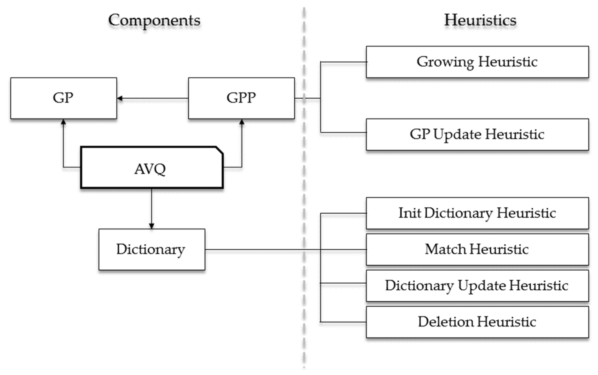
In Figure 2, we graphically highlight the logical architecture of the AVQ algorithm. As it is noticeable from this figure, the key elements can be subdivided into two distinct categories:
- Components;
- Heuristics.
A component is a data structure involved in the compression (or in the decompression) phase of the AVQ algorithm. The main components are the following:
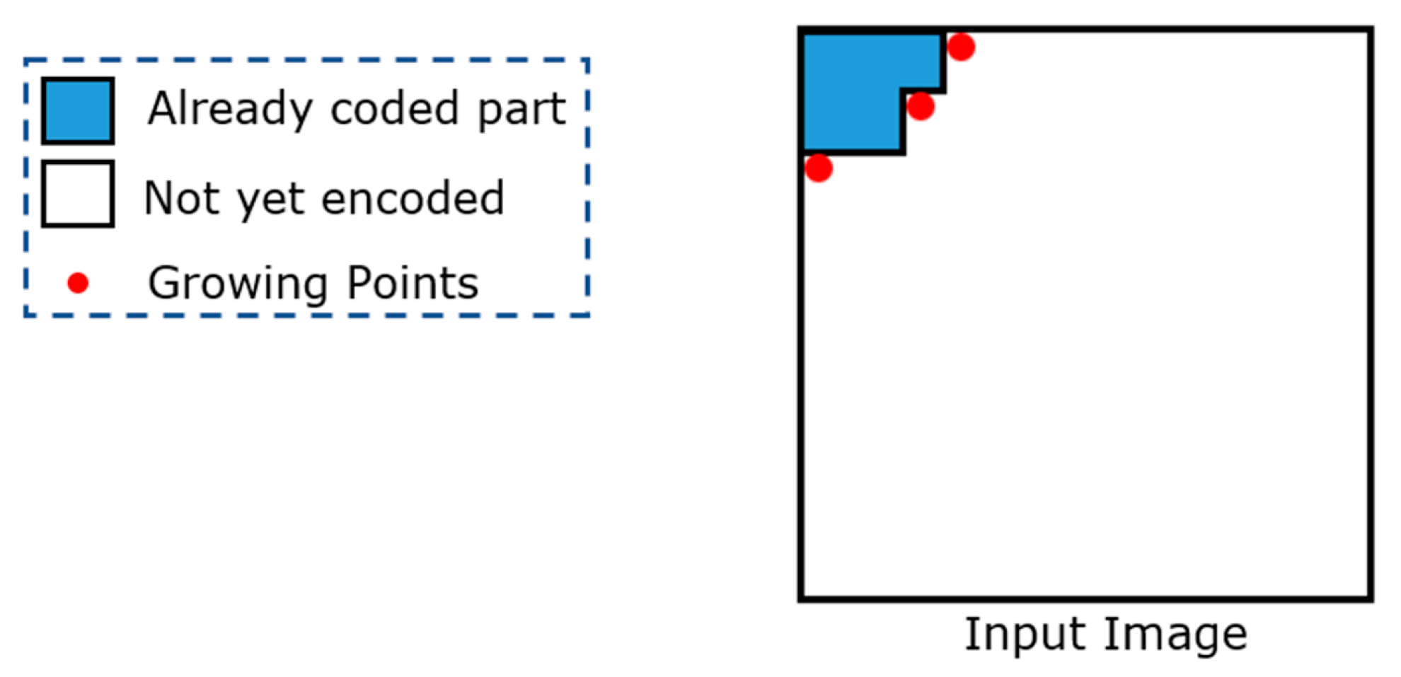
• Growing Points (GPs)
In contrast with one-dimensional data, two-dimensional data can have several uncoded points, from which an encoding algorithm can continue its encoding process. These points are referred to as growing points (GPs). Figure 3 shows a graphical example in which three GPs are highlighted in red.
The encoder selects one GP at each step and identifies a match between the block anchored to the selected GP (we denote the selected GP as gp from now on) and a similar block (according to a given distortion measure) contained in the dictionary. Therefore, by using the GPs, the AVQ algorithm can continue its encoding process in a deterministic manner.
• Growing Point Pool (GPP)
A GPP is a data structure in which all the Growing Points (GPs) are maintained.
• Dictionary (D)
All the blocks derived from the already coded parts of the input image are stored in the dictionary. Such blocks are used to find a match with a block (anchored to a GP) in the not yet coded portion of the input image. It should be noted that the dictionary plays an important role for the compression (and the decompression) of the input image.
We can informally define a heuristic as a set of rules that describes the behavior of the AVQ algorithm and its architectural element. Mainly, the heuristics are related to the GPP and the dictionary, and are the following:
• Growing Heuristic (GH)
A GH highlights the behavior related to the identification of the next GP, which will be extracted from the GPP. Such a GP will be the next one that will be processed by the AVQ algorithm. Several strategies can be adopted to define a GH. The ones used in literature are the following:
– Wave Growing Heuristic
The Wave GH selects a GP in which the coordinates, , satisfies the following relationship:
With this heuristic, the GPP is initialized in this manner: GPP . The point is the pixel at the left top corner. In addition, the image coverage follows perpendicular to the main diagonal by a wavelike trend.
– Diagonal Growing Heuristic
The Diagonal GH selects a GP in which the coordinates, , which satisfies the following relationship:
In this scenario, the GPP is initialized in the same way of the initialization of the Wave GH and the image coverage follows perpendicular to the main diagonal.
– LIFO Growing Heuristic
A GP is selected from the GPP in Last-In-First-Out (LIFO) order.
• Growing Point Update Heuristic (GPUH)
A GPUH defines the behavior related to the updating of the GPP. Indeed, a GPUH defines the set of adding one or more GP to the GPP.
• Init Dictionary Heuristic (IDH)
An IDH is a set of rules that define in which manner the dictionary, D, will be initialized.
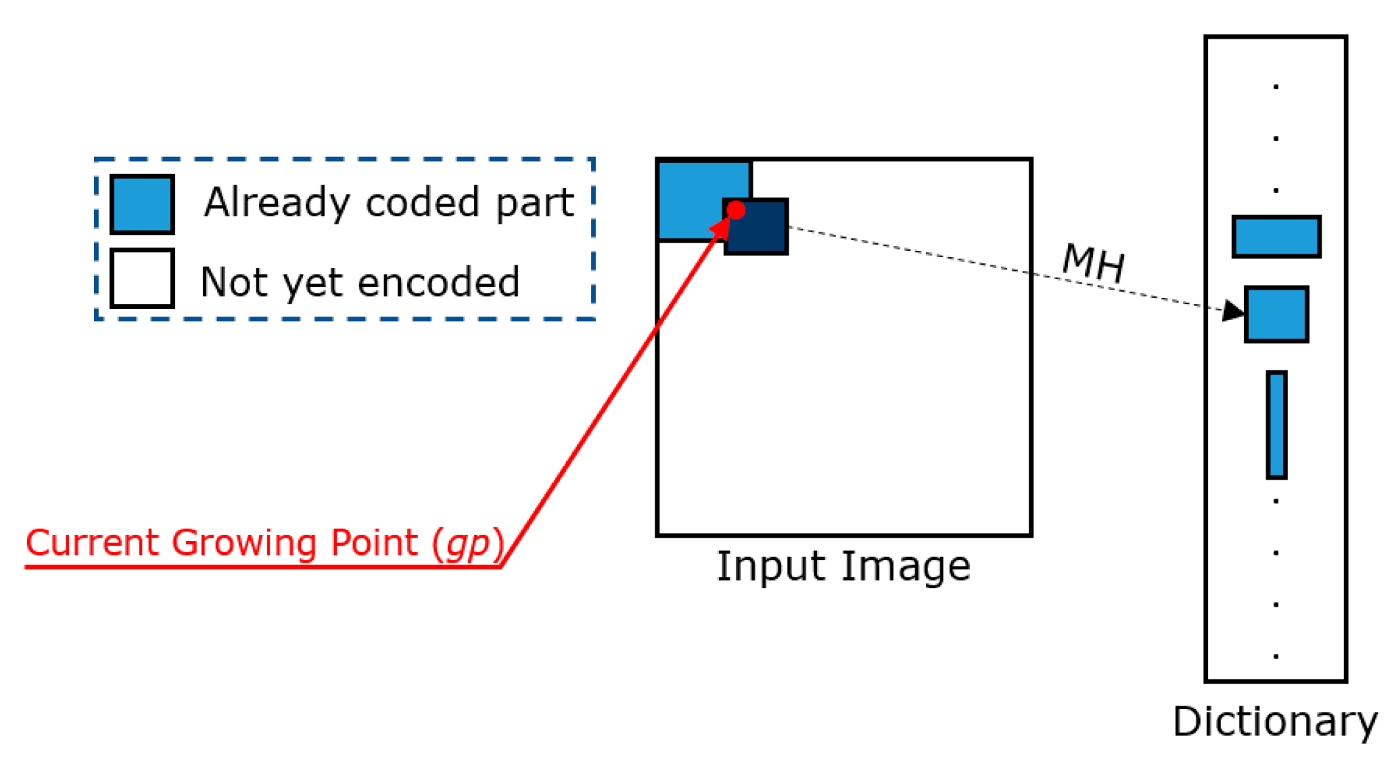
• Match Heuristic (MH)
An MH is used by the AVQ algorithm to identify a match between the block b, anchored to the GP that is undergoing the process (we referred to as gp), and a block in the dictionary D. Generally, a distance is used (e.g., Mean Squared Error - MSE [9], etc.) to define the similarity between a block in the dictionary and the block anchored to gp.
• Dictionary Update Heuristic (DUH)
A DUH is a set of rules that defines which new block(s) can be added to the dictionary D. Several DUH are explained in literature, as, for instance, the OneRow + OneColumn DUH (outlined in [5]). This heuristic adds two new blocks to the dictionary, if possible. The first block and the second block are obtained by adding a row to the matched block, in the already coded part of the image, as shown in Figure 4.
• Deletion Heuristic (DH)
A DH is used when all of the entries of the dictionary D are used. Such a heuristic defines which blocks in the dictionary should be deleted in order to make space.
2.2. Compression and Decompression Phases
Algorithm 1 highlights the pseudo-code of the AVQ compression phase. Firstly, the dictionary D and the GPP are initialized. The dictionary D is initialized by one entry for each value that a pixel can assume (i.e., in the case of grayscale images, D will be initialized with 256 values, from 0 to 255).
| Algorithm 1. Pseudo-code of the compression stage (AVQ algorithm). | |
| 1. | GPP ← Initial GPs (e.g., the at coordinates ) |
| 2. | D ← Use an IDH for the initialization |
| 3. | while GPP has more elements do |
| 4. | Use a GH to identify the next GP |
| 5. | Let gp be the current GP |
| 6. | Use an MH to find a block b in D that matches the sub- block anchored to gp |
| 7. | Transmit bits for the index of b |
| 8. | Update D with a DUH |
| 9. | if D is full then |
| 10. | Use a DH |
| 11. | endif |
| 12. | By using a GPUH, update the GPP |
| 13. | Remove gp from GPP |
| 14. | end while |
At each step, the AVQ algorithm selects a growing point from the growing point pool GPP (we referred to as gp), according to a specified growing heuristic (GH). The algorithm ends when there are no further selectable growing points (i.e., the GPP is empty).
Subsequently, the encoder uses a match heuristic (MH) to individuate which block, stored in the local dictionary D, is the best match for the one anchored to gp (see Figure 5). In general, the matching heuristics prefer the largest block in D, which presents a distortion measure that is less than or equal to a threshold T, when compared with the block anchored to gp. The threshold T can be fixed for the whole image or can be dynamically adjusted by considering the image content, in order to improve the quality perception.
Once the match is performed and a block in D is identified, the index of this block (denoted as b in Algorithm 1) can be stored or transmitted. An index can be represented with bits ( is the size of the dictionary D). After that, the dictionary D is updated, by adding one or more blocks to it. The update is directed by the rules defined by a dictionary update heuristic (DUH). If D is full, a deletion heuristic (DH) is invoked to eventually make space in D.
Finally, the GPP is also updated by using a growing update heuristic (GUH). The processed growing point (i.e., gp) is removed from the GPP. Thus, such a growing point will not be further processed.
It is important to point out that the compression performances are strictly dependent on the number of indexes that will be stored or transmitted by the encoder. Indeed, by considering that each block is represented by its index in the dictionary, more blocks will be necessary to cover the input image, and it will be necessary for more indices to be stored or transmitted. Vice versa, less blocks will be necessary to cover the input image, and it will be necessary for less indices to be stored or transmitted. Consequently, even the dimensions of the matched blocks can influence the compression performances. In fact, the matched blocks with larger dimensions can increase the compression performances, since they cover larger portions of the input image.
Algorithm 2 reports the pseudo-code related to the AVQ decompression phase. Substantially, the pseudo-code is symmetrical, except for the fact that the decompression phase does not need to identify the match, since it receives the indices from the encoder (or reads the indices from a file).
| Algorithm 2. Pseudo-code of the decompression stage (AVQ algorithm). | |
| 1. | GPP ← Initial GPs (e.g., the at coordinates ) |
| 2. | D ← Use an IDH for the initialization |
| 3. | while GPP has more elements do |
| 4. | Use a GH to identify the next GP |
| 5. | Let gp be the current GP |
| 7. | Receive bits representing the index of a block b into the dictionary D |
| Anchor b to the current GP, gp, in order to reconstruct the output image | |
| 8. | Update D with a DUH |
| 9. | if D is full then |
| 10. | Use a DH |
| 11. | endif |
| 12. | By using a GPUH, update the GPP |
| 13. | Remove gp from GPP |
| 14. | end while |
In Figure 6a, we graphically show, in false-colors, the progress of Algorithm 1, on the image denoted as Lena. In detail, each block visually indicates the dimensions of the corresponding block, identified in the dictionary D. In Figure 6b, we graphically show the progress of the decompression phase (Algorithm 2).
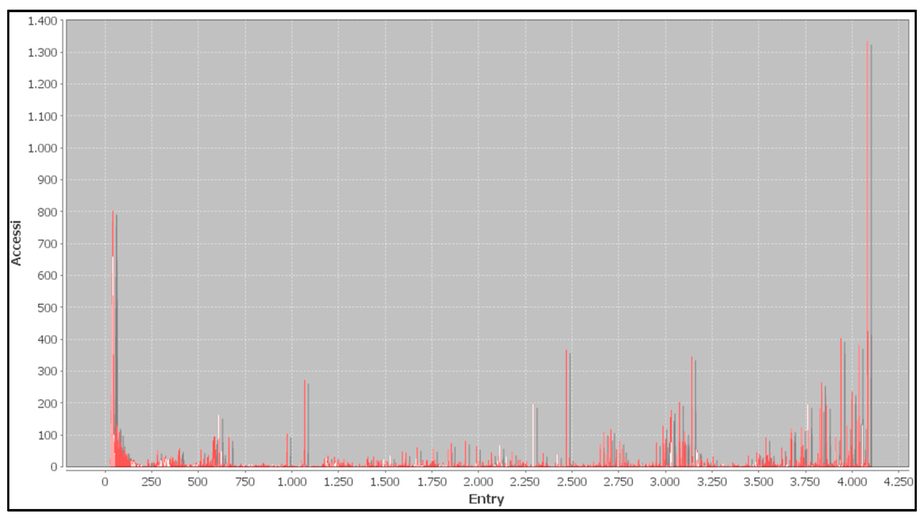
The graph in Figure 7 shows the number of access (on the y-axis) to a specific index of the dictionary D (on the x-axis), during the compression phase.
3. The AVQ for Image Sequences (AVQIS) Algorithm
In this section, we focus on the description of an easy-to-implement extension of the AVQ algorithm, which allows the lossy compression of image sequences, without influencing the execution time of the algorithm (for both compression and decompression phases). The extension is easily implementable and requires only few modifications, starting from an existing AVQ implementation.
We emphasize that by compressing, in an independent manner, each frame of an image sequence IS through the AVQ algorithm, only the spatial correlation (i.e., the correlation within the same frame) is exploited. Indeed, during the encoding of the i-th frame of IS, the AVQ algorithm will use only the blocks derived from the already coded part of the i-th frame itself.
Our objective is to extend the AVQ algorithm to exploit also the temporal correlation among the frames of an image sequence, by minimizing the effort for the modifications of an existing AVQ implementation. Therefore, we considered using a dictionary (we referred to as shared dictionary), that will be shared during the processing of all of the input frames (frame1, …, framei, …, frameN) of an image sequence IS [10].
The main benefit that provides a shared dictionary (SD) is related to the fact that it hosts the blocks derived from the coded portions of the input frame as well as the ones derived from previously coded frames. Therefore, the encoder has a greater probability to individuate matched blocks with larger dimensions, which can cover larger areas of the input frame and, consequently, the compression performances should be improved. On the other hand, the perceivable quality of the compressed frames could be lower with respect to the usage of a local independent dictionary for each frame, since some blocks are obtained by previous coded frames and present a slightly lower similarity.
Starting from these considerations, we outline a novel scheme based on the AVQ algorithm, which we refer to as Adaptive Vector Quantization for Image Sequences (AVQIS). AVQIS can be used for lossy compression of image sequences. In order to maintain a high degree of ease of implementation, the existing heuristics are the same as the ones involved in the AVQ algorithm. Consequently, the blocks stored in the shared dictionary will be treated in the same manner whether they were obtained from the current frame or whether they were obtained from the previously encoded frames.
In Algorithm 3, we report the pseudo-code related to the compression stage of the AVQIS algorithm. In detail, each one of the N frames of IS (the input image sequence) is compressed through the fAVQ algorithm. The fAVQ algorithm is directly derived from the AVQ algorithm and is able to operate on the shared dictionary SD, instead of the local dictionary D. As it is possible to observe in Figure 8, the shared dictionary SD is involved among the instances of the fAVQ algorithm (one instance per frame). We remark that during the compression of the i-th frame framei (i > 0), by the fAVQ algorithm, the SD contains blocks from the already coded parts of the frame in process (i.e., framei) and from the previous coded frames (framej, j = 1, …, i − 1).
| Algorithm 3. Pseudo-code of the compression stage (AVQIS algorithm). | |
| 1. | SD ← Use an IDH for the initialization |
| 2. | for i ← 1 to N do |
| 3. | framei ← i-th frame of IS |
| 4. | frameiC ← fAVQCompression(framei, SD) |
| 5. | end for |
| 6. | ISC ←{ frame1C, …, frameiC, …, frameNC} |
In Algorithm 4, we outline the pseudo-code of the decompression stage. It should be noted that the decompression stage is substantially symmetrical with respect to the compression one.
| Algorithm 4. Pseudo-code of the decompression stage (AVQIS algorithm). | |
| 1. | SD ← Use an IDH for the initialization |
| 2. | for i ← 1 to N do |
| 3. | frameiC ← i-th frame of ISC |
| 4. | framei ← fAVQDecompression(frameiC, SD) |
| 5. | end for |
| 6. | IS ←{ frame1, …, framei, …, frameN} |
4. Experimental Results
The main objective of our experiments is to compare the compression performances, in terms of Compression Ratio (C.R.), between the AVQ algorithm (in which each frame is independently compressed) and the AVQIS algorithm. In addition, we measure the Peak-Signal-to-Noise-Ratio (PSNR) metric, in order to compare the perceptive quality. It is important to outline that the execution times we have achieved in our experiments are comparable between the two algorithms.
We used two datasets (we referred to as Dataset 1 and Dataset 2, respectively), each one composed of three image sequences. Dataset 1 is composed of image sequences extracted from a video, while three infrared image sequences compose Dataset 2.
4.1. Dataset 1
The first dataset we consider (Dataset 1) is composed of three image sequences. In Table 1, we report a short description. All the sequences are publicly available at [11]. In the following, for brevity, we refer to an image sequence of Dataset 1, by using a short name (reported in the second column of Table 1).
The parameters we used for our experiments are the following:
- Wave Heuristic as Growing Heuristic;
- OneRow+OneColumn as Dictionary Update Heuristic;
- Freeze as Deletion Heuristic;
- MSE-based as Match Heuristic (threshold value equal to 10).
The dictionary is initialized with all of pixels for continuous grayscale (IDH), and we set the size of the dictionary (AVQ) as well as the shared dictionary (AVQIS) of 16384 (214).
In Figure 9, we report a graphical comparison of the achieved experimental results, in terms of Compression Ratio (C.R.), reported on the y-axis, achieved by the AVQ algorithm (blue line) and the AVQIS algorithm (red line) for all of the frames (on the x-axis) of the three image sequences.
4.2. Results Analysis (Dataset 1)
Table 2 synthetizes the achieved average results, in terms of C.R. The second and third columns of Table 2, report the AVQ and the AVQIS achieved average results, respectively. The results are reported for each one of the image sequences of Dataset 1 (first column).
From such a table, it is noticeable that the compression performances of the AVQIS algorithm are better, with respect to the AVQ algorithm, in two cases: Seq. 1 and Seq. 3. In relation to the sequence referred to as Seq. 2, the AVQIS algorithm achieves slightly worse performance. Indeed, the AVQIS algorithm achieves an average C.R. of 2.41, while the AVQ algorithm achieves an average C.R. of 2.44.
In Figure 10, we graphically report the trends of the achieved PSNR metric for each one of the image sequences of Dataset 1, in relation to the AVQ algorithm (green line) and the AVQIS algorithm (magenta line). From Table 3, which synthetizes the achieved average PSNR, it is noticeable that the AVQ algorithm achieves a better PSNR for the Seq. 2 and Seq. 3 sequences, while, in Seq. 1, the AVQIS algorithm obtains a higher PSNR. In Table A1,
4.3. Dataset 2
Dataset 2 is composed of three infrared image sequences and is briefly described in Table 4 (further details in [12]).
The parameters we used for our experiments are the following:
- Wave Heuristic as Growing Heuristic;
- OneRow+OneColumn as Dictionary Update Heuristic;
- Freeze as Deletion Heuristic;
- MSE-based as Match Heuristic (threshold value equal to 5.5).
Finally, the dictionary is initialized with all pixels for continuous grayscale (IDH). Furthermore, we set the size of the dictionary (AVQ) as well as the shared dictionary (AVQIS) as 4096 (212) and 8192 (213), respectively.
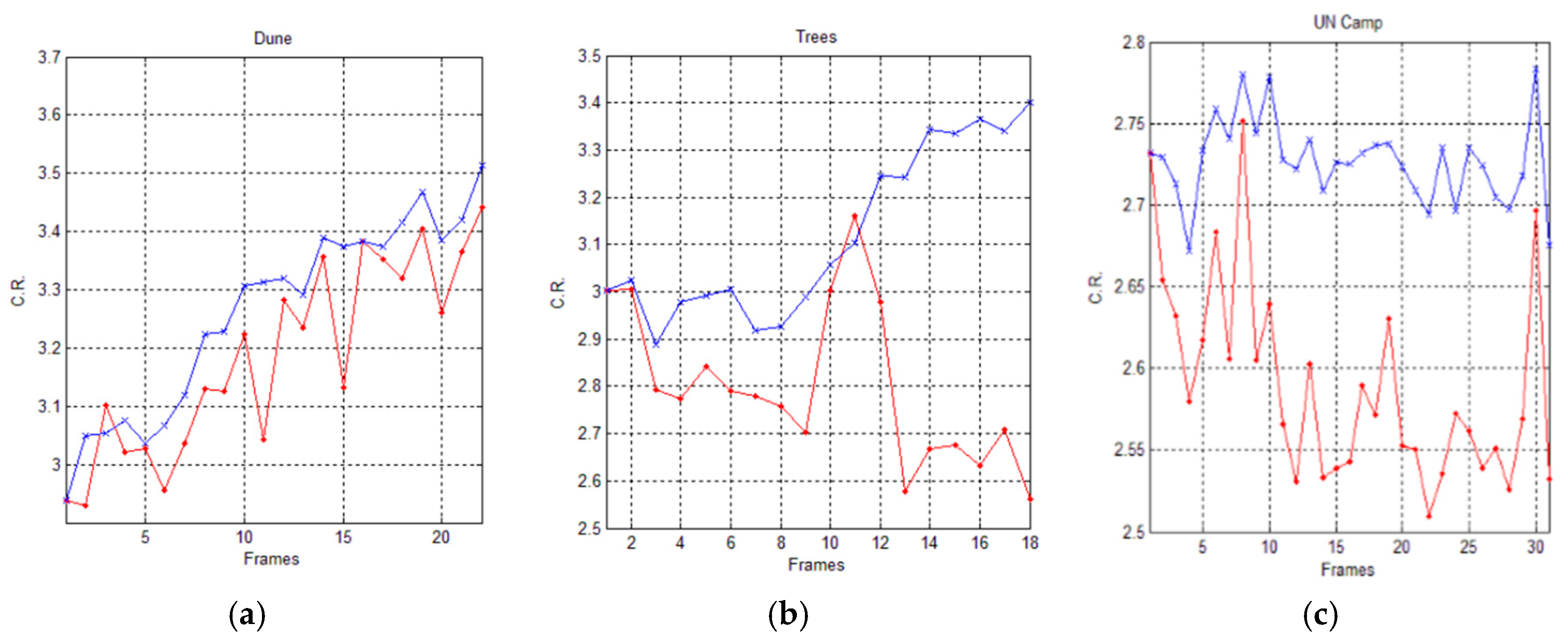
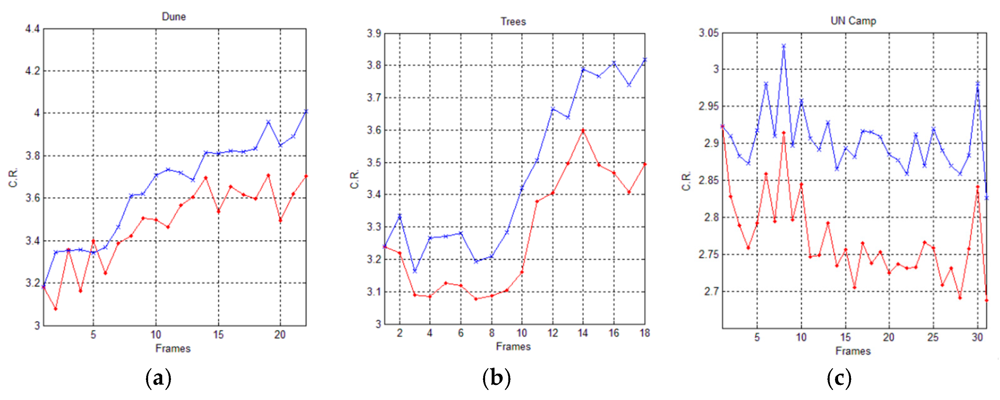
In Figure 11 and Figure 12, we graphically compare the experimental results, in terms of Compression Ratio (C.R.), achieved by the AVQ algorithm (blue line) and the AVQIS algorithm (red line), by considering the size of the dictionary/shared dictionary of 4096 (212) entries and of 8192 (214), respectively.
4.4. Results Analysis (Dataset 2)
Table 5 and Table 6 summarize the achieved average C.R. when AVQ (second column) and AVQIS (third column) are used, for each one of the used image sequences (first column). From these tables, it is possible to observe that the compression performances of the AVQIS algorithm are better with respect to the AVQ algorithm in all of the tested sequences.
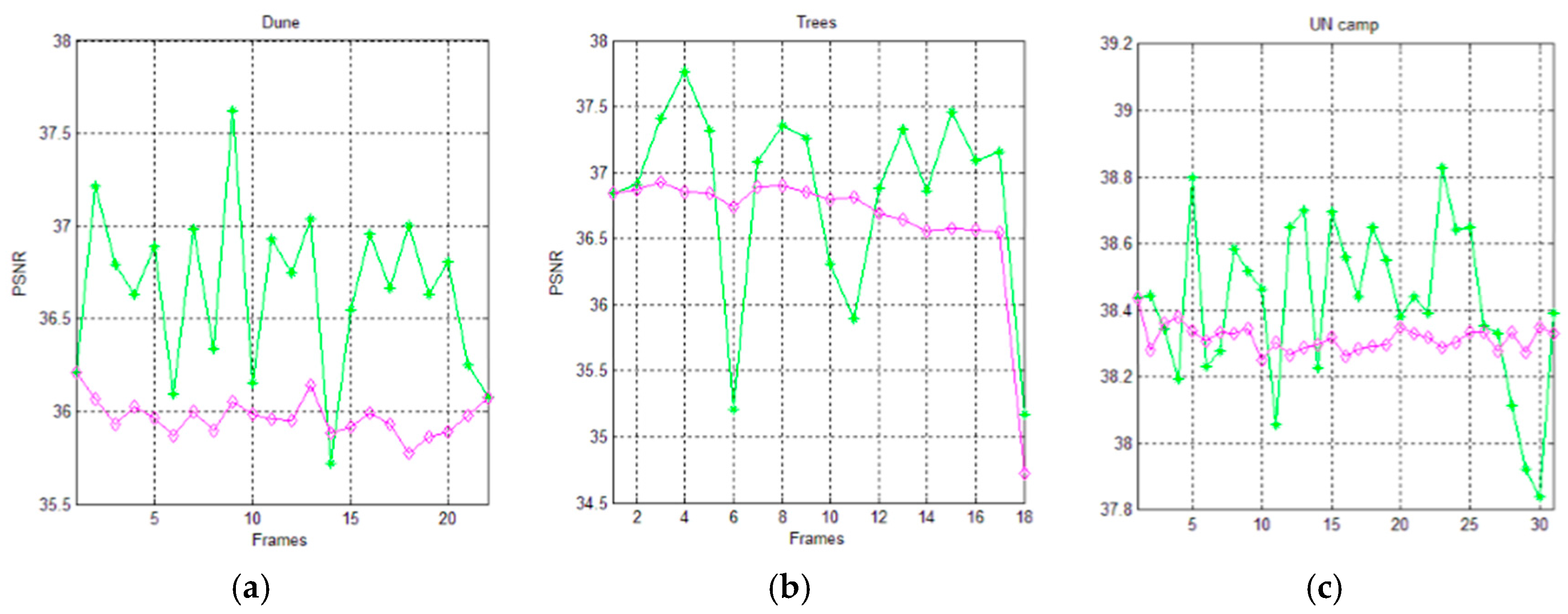
Figure 13 and Figure 14 show the trends of the PSNR metric for the AVQ algorithm (green line) and the AVQIS algorithm (magenta line) when dictionaries of 4096 entries and of 8192 entries are used, respectively. As is observable from these figures and from Table 7 and Table 8, which summarize the achieved average PSNRs, the trend obtained by the AVQIS algorithm is generally slightly worse, except for a few cases (e.g., the 14-th frame of the sequence denoted as “Dune”).
5. Conclusions
In this work, we propose a lossy compression scheme for image sequences, based on the AVQ algorithm, which we denoted as AVQIS. Our approach uses a shared dictionary to exploit the temporal correlation of image sequences.
The experimental results that we achieved show slight improvements, on average, in terms of compression performances, when the AVQIS algorithm is compared with the AVQ algorithm. However, we have designed our approach in order for it to be easily implementable and it does not affect the execution time. The compression performances are dependent anyway on the temporal correlation among the frames that compose the input image sequence.
Future research directions will include the testing on collections of bi-level images [13] and on 3D medical images [14]. Moreover, we will focus on the design of new heuristics and on the design of parallel implementations through adequate frameworks (e.g., the OpenCL framework [15], etc.) of the AVQIS algorithm (e.g., based on the technique addressed in [16]). In addition, we will focus on a possible pre-processing based on a frame ordering (similar to the one highlighted in [17]), which could improve the compression performances.
Acknowledgments
The authors would like to thank students Vincenzo Fariello and Andrea Vallati, who have implemented and tested a preliminary version of the AVQIS algorithm.
Author Contributions
Raffaele Pizzolante designed and performed the experiments. Raffaele Pizzolante, Bruno Carpentieri and Sergio De Agostino wrote the paper.
Conflicts of Interest
The authors declare no conflict of interest.
Appendix
In Table A1, Table A2 and Table A3, we respectively report three uncompressed frames of Seq. 1 (Table A1), Seq. 2 (Table A2) and Seq. 3 (Table A3) of Dataset 1, and the same frames obtained as output of the compression, by using the AVQ algorithm and the AVQIS algorithm.

Table A1.
Example of some frames from Seq. 1-Dataset 1. Appendix.
| Frame No. | 1 | 9 | 15 |
|---|---|---|---|
| Uncompressed |  |  |  |
| AVQ |  |  |  |
| AVQIS |  |  |  |
Table A2.
Example of some frames from Seq. 2-Dataset 1.
| Frame No. | 1 | 15 | 30 |
|---|---|---|---|
| Uncompressed |  |  |  |
| AVQ |  |  |  |
| AVQIS |  |  |  |
Table A3.
Example of some frames from Seq. 3-Dataset 1.
| Frame No. | 3 | 6 | 9 |
|---|---|---|---|
| Uncompressed |  |  |  |
| AVQ |  |  |  |
| AVQIS |  |  |  |
References
- Valsesia, D.; Boufounos, P. Multispectral image compression using universal vector quantization. In Proceedings of the Multispectral Image Compression Using Universal Vector Quantization, Cambridge, UK, 11–14 September 2016; Information Theory Workshop (ITW): Cambridge, UK, 2016. [Google Scholar]
- Ryan, M.J.; Arnold, J.F. The lossless compression of AVIRIS images by vector quantization. IEEE Trans. Geosci. Remote Sens. 1997, 35, 546–550. [Google Scholar] [CrossRef]
- Kekre, H.B.; Prachi, N.; Tanuja, S. Color image compression using vector quantization and hybrid wavelet transform. In Proceedings of the Computer Science 89, Bangalore, India, 19–21 August 2016; pp. 778–784. [Google Scholar]
- Gersho, A.; Gray, R.M. Vector Quantization and Signal Compression; Kluwer Academic Press: Dordrecht, The Netherlands, 1992. [Google Scholar]
- Constantinescu, C.; Storer, J.A. Improved techniques for single-pass adaptive vector quantization. Proc. IEEE 1994, 82, 933–939. [Google Scholar] [CrossRef]
- Ziv, J.; Lempel, A. Compression of individual sequences via variable-length coding. IEEE Trans. Inf. Theory 1978, 24, 530–536. [Google Scholar] [CrossRef]
- Carpentieri, B. Image compression via textual substitution. Wseas Trans. Inf. Sci. Appl. 2009, 6, 768–777. [Google Scholar]
- Sheinwald, D.; Lempel, A.; Ziv, J. Two-dimensional encoding by finite state encoders. IEEE Trans. Commun. 1990, 38, 341–347. [Google Scholar] [CrossRef]
- DeGroot, M.H.; Schervish, M.J. Probability and Statistics, 4th ed.; Addison Wesley: Boston, MA, USA, 2011. [Google Scholar]
- Pizzolante, R. Lossy compression of image sequences through the AVQ algorithm. In Proceedings of the International Conference on Data Compression, Communication Processing and Security, Salerno, Italy, 22–23 September 2016. [Google Scholar]
- SIPI Image Sequences. Available online: http://sipi.usc.edu/database/database.php?volume=sequences (accessed on 6 May 2017).
- Lewis, J.J.; Nikolov, S.G.; Canagarajah, C.N.; Bull, D.R.; Toet, A. Uni-modal versus joint segmentation for region-based image fusion. IEEE 9th International Conference on Information Fusion, Florence, Italy, 10–13 July 2006; pp. 1–8. [Google Scholar]
- De Agostino, S. Compressing Bi-level images by block matching on a tree architecture. In Proceedings of the Prague Stringology conference 2009, Prague, Czech Republic, 31 August–2 September 2009. [Google Scholar]
- Pizzolante, R.; Carpentieri, B.; Castiglione, A. A secure low complexity approach for compression and transmission of 3-D medical images. Proceeding of the 2013 Eighth International Conference on Broadband and Wireless Computing, Communication and Applications, Compiegne, France, 28–30 October 2013; pp. 387–392. [Google Scholar]
- Pizzolante, R.; Castiglione, A.; Carpentieri, B.; de Santis, A. parallel low-complexity lossless coding of three-dimensional medical images. Proceeding of the NBIS 2014 17th International Conference on Network-Based Information Systems, 10–12 September 2014; pp. 91–98. [Google Scholar]
- Cinque, L.; Agostino, S.D.; Lombardi, L. Practical parallel algorithms for dictionary data compression. In Proceedings of the 2009 Data Compression Conference, Snowbird, UT, USA, 16–18 March 2009; p. 441. [Google Scholar]
- Pizzolante, R.; Carpentieri, B. Visualization, band ordering and compression of hyperspectral images. Algorithms 2012, 5, 76–97. [Google Scholar] [CrossRef]
Figure 1.
The usage of the VQ by an encoder (a) and by a decoder (b).
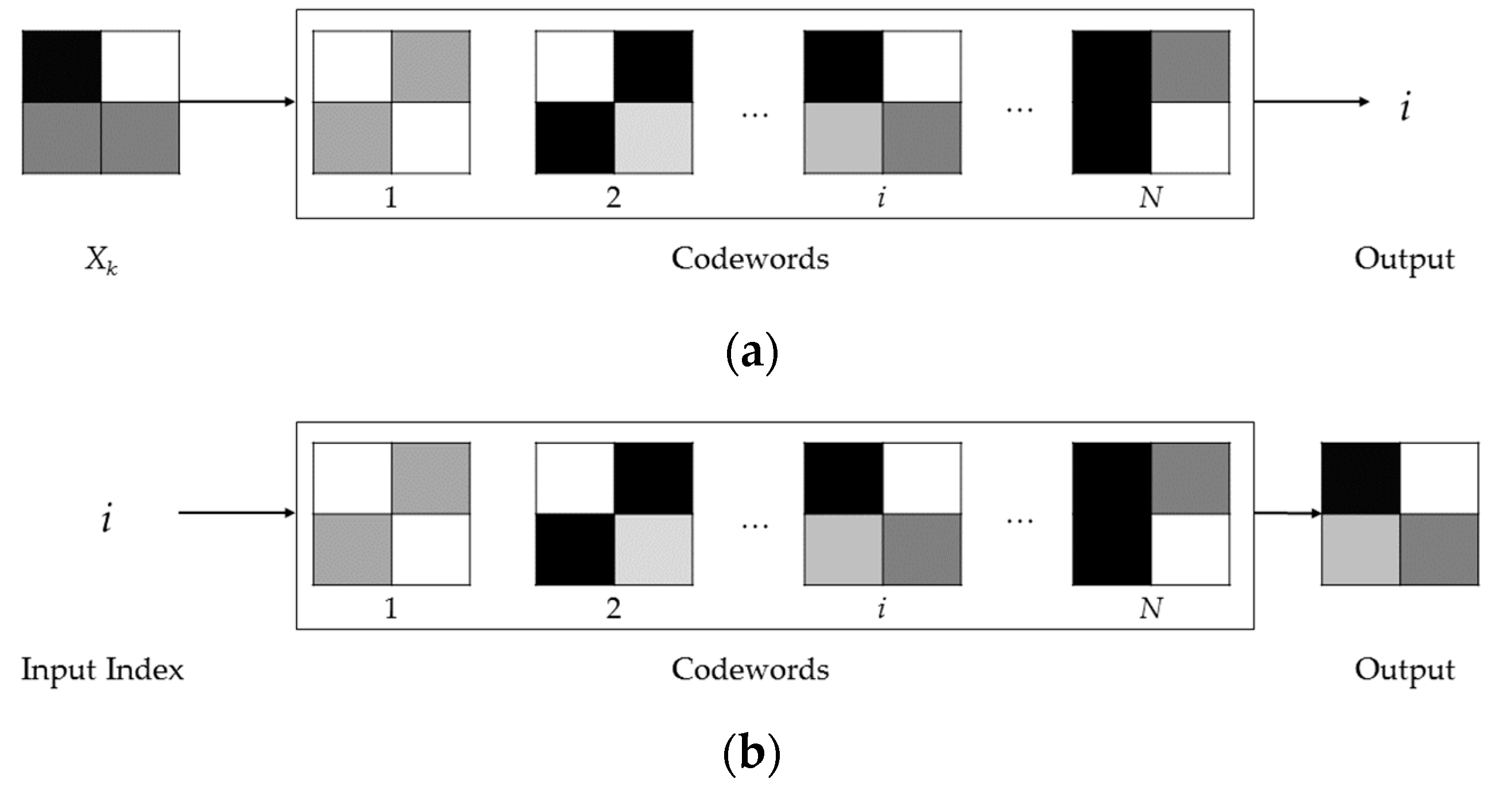
Figure 2.
The block diagram of the architecture of the AVQ algorithm.

Figure 3.
Examples of growing points.

Figure 4.
An example of the OneRow+OneColumn Dictionary Update Heuristic. (a) The matched block; (b) The first added block into the dictionary; (c) The second block added into the dictionary.
Figure 4.
An example of the OneRow+OneColumn Dictionary Update Heuristic. (a) The matched block; (b) The first added block into the dictionary; (c) The second block added into the dictionary.
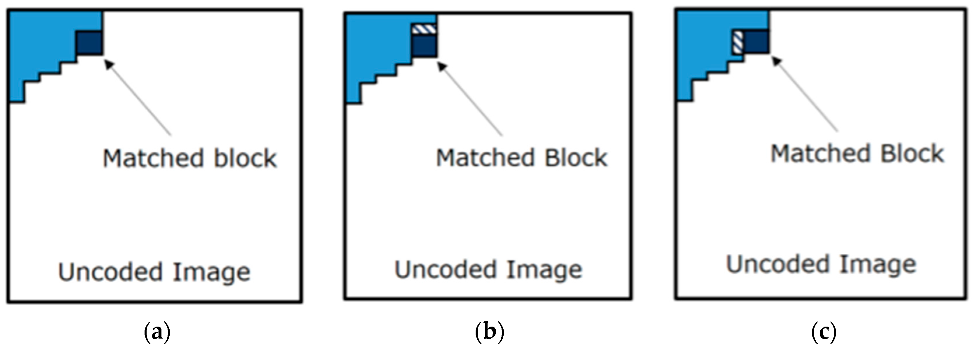
Figure 5.
Examples of matching heuristics.

Figure 6.
Graphical representation of: (a) the progress (in false-colors) of the compression stage; (b) the progress of the decompression stage.
Figure 6.
Graphical representation of: (a) the progress (in false-colors) of the compression stage; (b) the progress of the decompression stage.
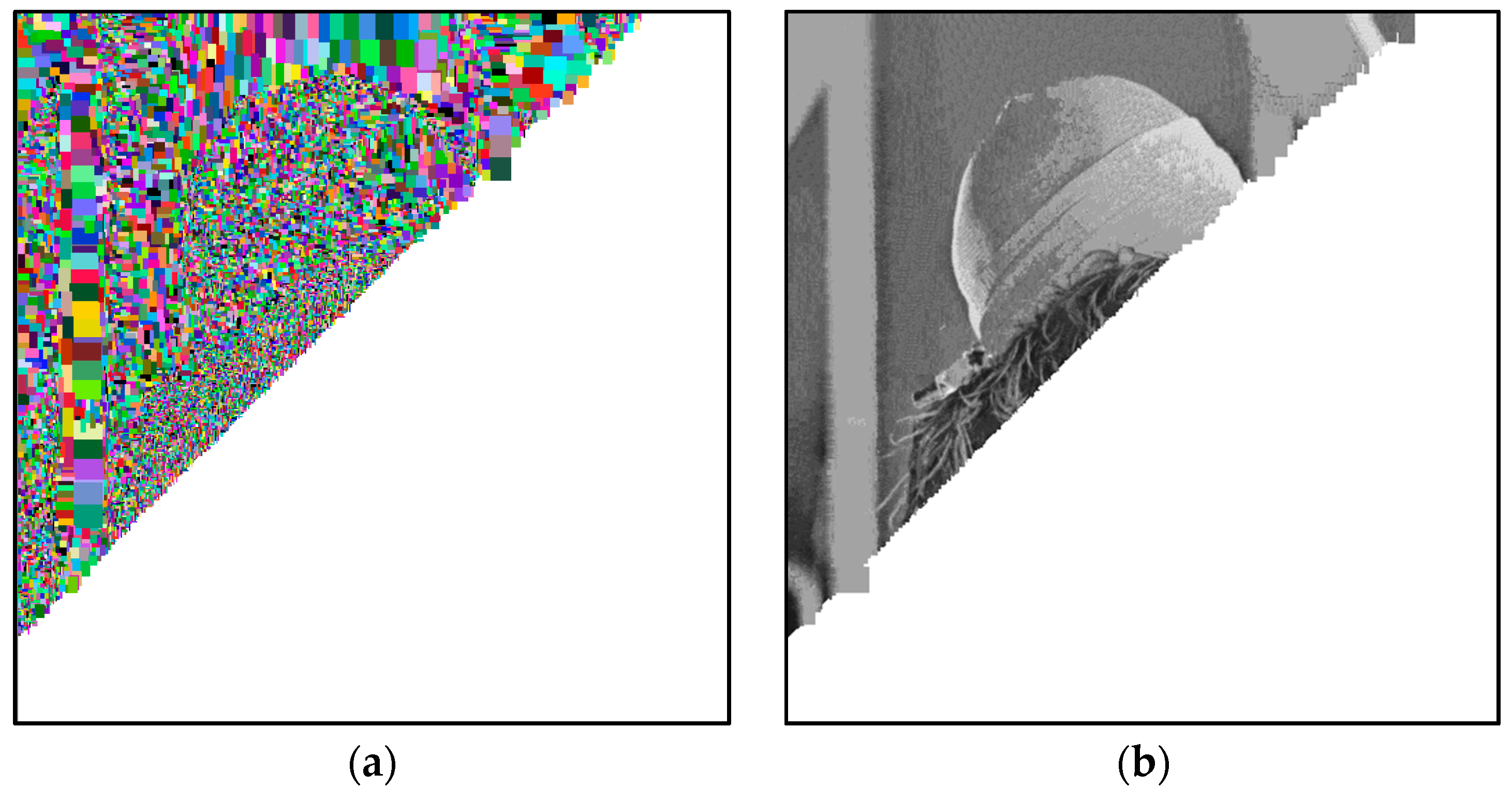
Figure 7.
Graphical representation of the number of access (on the y-axis) to a specific index of the dictionary (on the x-axis) during the compression phase.
Figure 7.
Graphical representation of the number of access (on the y-axis) to a specific index of the dictionary (on the x-axis) during the compression phase.

Figure 8.
The shared dictionary used by each one of the fAVQ instances.
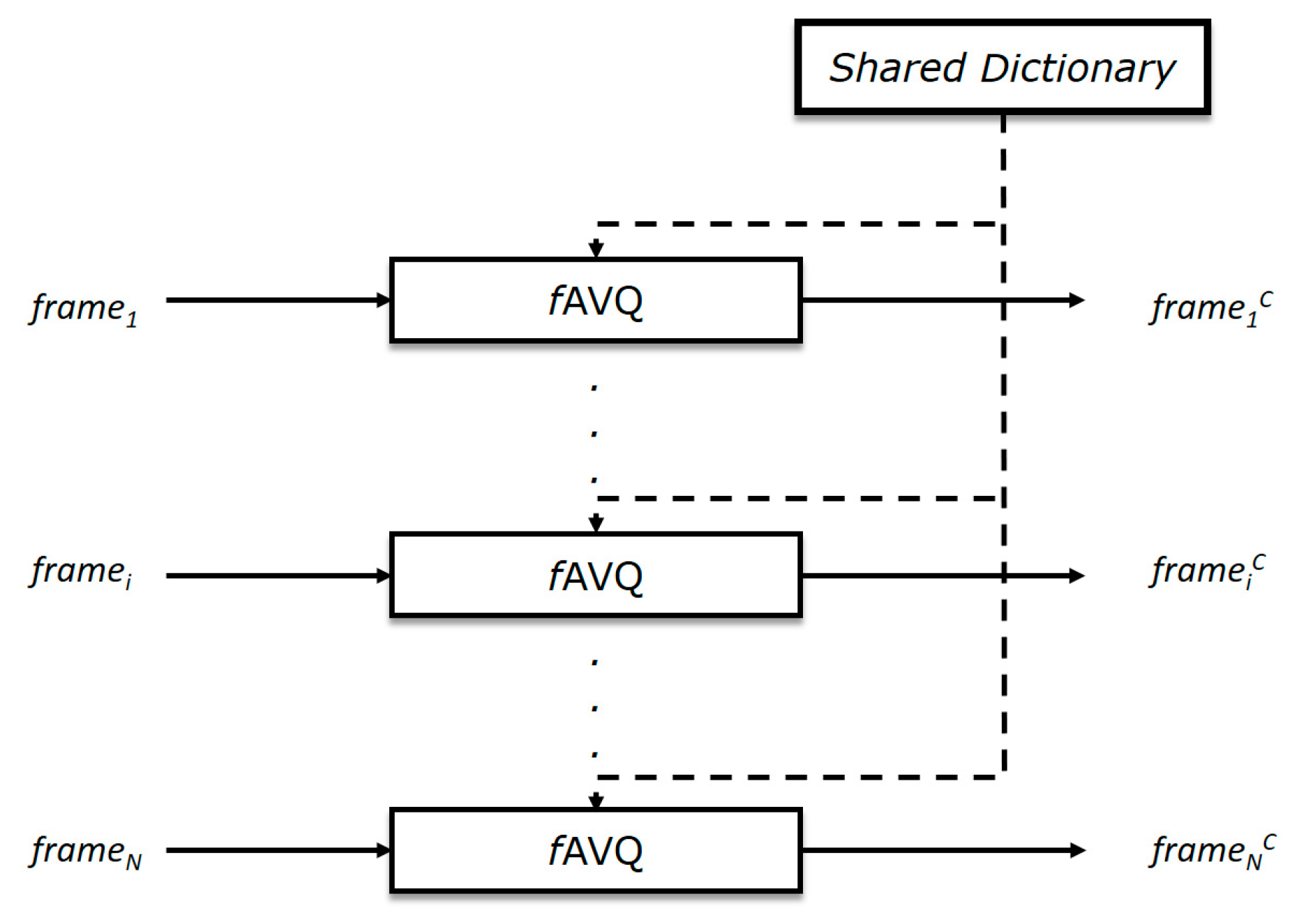
Figure 9.
Graphical comparison of the achieved C.R. between the AVQIS algorithm (blue line) and the AVQ algorithm (red line) for (a) Seq. 1; (b) Seq. 2; and (c) Seq. 3.
Figure 9.
Graphical comparison of the achieved C.R. between the AVQIS algorithm (blue line) and the AVQ algorithm (red line) for (a) Seq. 1; (b) Seq. 2; and (c) Seq. 3.
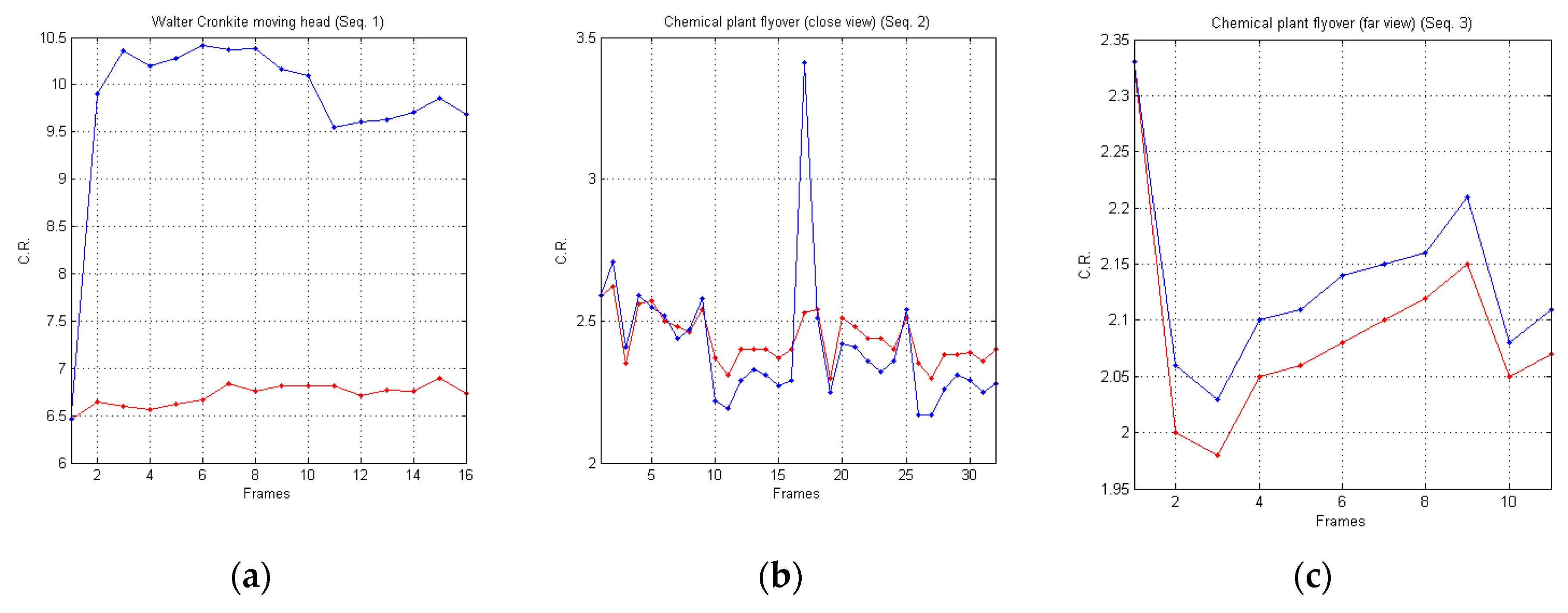
Figure 10.
Graphical comparison of the achieved PSNR between the AVQ algorithm (green line) and the AVQIS algorithm (magenta line), for (a) Seq. 1; (b) Seq. 2; and (c) Seq. 3.
Figure 10.
Graphical comparison of the achieved PSNR between the AVQ algorithm (green line) and the AVQIS algorithm (magenta line), for (a) Seq. 1; (b) Seq. 2; and (c) Seq. 3.
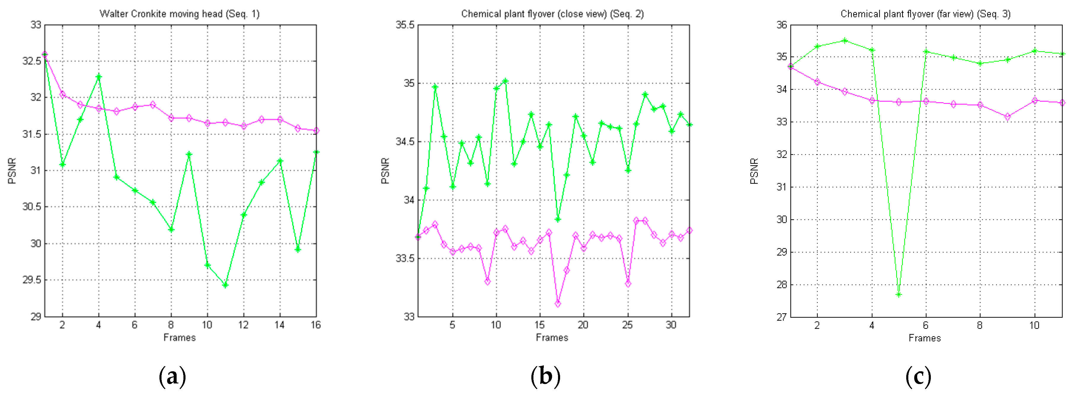
Figure 11.
Graphical comparison of the achieved C.R. between the AVQIS algorithm (blue line) and the AVQ algorithm (red line), by using a dictionary of 4096 (212), for (a) the Dune sequence; (b) the Trees sequence; and (c) the UN camp sequence.
Figure 11.
Graphical comparison of the achieved C.R. between the AVQIS algorithm (blue line) and the AVQ algorithm (red line), by using a dictionary of 4096 (212), for (a) the Dune sequence; (b) the Trees sequence; and (c) the UN camp sequence.

Figure 12.
Graphical comparison of the achieved C.R. between the AVQIS algorithm (blue line) and the AVQ algorithm (red line), by using a dictionary of 8192 (213) entries, for (a) the Dune sequence; (b) the Trees sequence; and (c) the UN camp sequence.
Figure 12.
Graphical comparison of the achieved C.R. between the AVQIS algorithm (blue line) and the AVQ algorithm (red line), by using a dictionary of 8192 (213) entries, for (a) the Dune sequence; (b) the Trees sequence; and (c) the UN camp sequence.

Figure 13.
Graphical comparison of the achieved PSNR between the AVQ algorithm (green line) and the AVQIS algorithm (magenta line), by using a dictionary of 4096 (212) entries, for (a) the Dune sequence; (b) the Trees sequence; and (c) the UN camp sequence.
Figure 13.
Graphical comparison of the achieved PSNR between the AVQ algorithm (green line) and the AVQIS algorithm (magenta line), by using a dictionary of 4096 (212) entries, for (a) the Dune sequence; (b) the Trees sequence; and (c) the UN camp sequence.
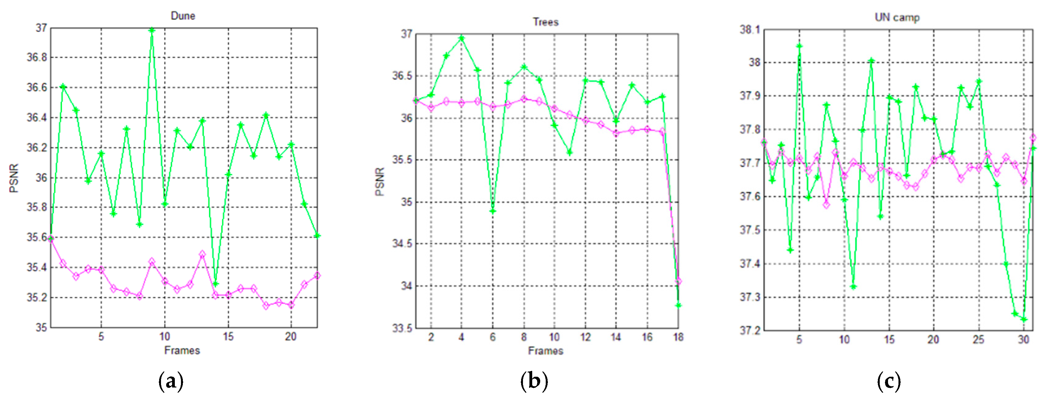
Figure 14.
Graphical comparison of the achieved PSNR between the AVQ algorithm (green line) and the AVQIS algorithm (magenta), by using a dictionary of 8192 (213) entries, for (a) the Dune sequence; (b) the Trees sequence; and (c) the UN camp sequence.
Figure 14.
Graphical comparison of the achieved PSNR between the AVQ algorithm (green line) and the AVQIS algorithm (magenta), by using a dictionary of 8192 (213) entries, for (a) the Dune sequence; (b) the Trees sequence; and (c) the UN camp sequence.

Table 1.
Dataset 1 description.
| Name | Short Name | Resolution | # of Frames |
|---|---|---|---|
| Walter Cronkite moving head | Seq. 1 | 16 | |
| Chemical plant flyover (close view) | Seq. 2 | 32 | |
| Chemical plant flyover (far view) | Seq. 3 | 11 |
Table 2.
Average C.R.–Dataset 1.
| Image Sequence/Average PSNR | AVQ | AVQIS |
|---|---|---|
| Seq. 1 | 6.72 | 9.79 |
| Seq. 2 | 2.41 | 2.44 |
| Seq. 2 | 2.09 | 2.13 |
Table 3.
Average PSNR–Dataset 1.
| Image Sequence/Average PSNR | AVQ | AVQIS |
|---|---|---|
| Seq. 1 | 30.87 | 31.80 |
| Seq. 2 | 34.51 | 33.62 |
| Seq. 2 | 34.42 | 33.75 |
Table 4.
Dataset 2 description.
| Name | Resolution | # of Frames |
|---|---|---|
| Dune | 22 | |
| Trees | 18 | |
| UN camp | 31 |
Table 5.
Average C.R. (dictionary composed by 4096 entries)–Dataset 2.
| Image Sequence/Average C.R. | AVQ | AVQIS |
|---|---|---|
| Dune | 3.18 | 3.26 |
| Trees | 2.80 | 3.12 |
| UN camp | 2.59 | 2.73 |
Table 6.
Average C.R. (dictionary composed by 8192 entries)–Dataset 2.
| Image Sequence/Average C.R. | AVQ | AVQIS |
|---|---|---|
| Dune | 3.48 | 3.65 |
| Trees | 3.28 | 3.47 |
| UN camp | 2.77 | 2.90 |
Table 7.
Average PSNR (dictionary composed by 4096 entries)–Dataset 2.
| Image Sequence/Average PSNR | AVQ | AVQIS |
|---|---|---|
| Dune | 36.65 | 35.97 |
| Trees | 36.85 | 36.65 |
| UN camp | 38.32 | 38.32 |
Table 8.
Average PSNR (dictionary composed by 8192 entries)–Dataset 2.
| Image Sequence/Average PSNR | AVQ | AVQIS |
|---|---|---|
| Dune | 36.10 | 35.30 |
| Trees | 36.11 | 35.95 |
| UN camp | 37.71 | 37.69 |
© 2017 by the authors. Licensee MDPI, Basel, Switzerland. This article is an open access article distributed under the terms and conditions of the Creative Commons Attribution (CC BY) license (http://creativecommons.org/licenses/by/4.0/).
Share and Cite
MDPI and ACS Style
Pizzolante, R.; Carpentieri, B.; De Agostino, S. Adaptive Vector Quantization for Lossy Compression of Image Sequences . Algorithms 2017, 10, 51. https://doi.org/10.3390/a10020051
AMA Style
Pizzolante R, Carpentieri B, De Agostino S. Adaptive Vector Quantization for Lossy Compression of Image Sequences . Algorithms. 2017; 10(2):51. https://doi.org/10.3390/a10020051
Chicago/Turabian StylePizzolante, Raffaele, Bruno Carpentieri, and Sergio De Agostino. 2017. "Adaptive Vector Quantization for Lossy Compression of Image Sequences " Algorithms 10, no. 2: 51. https://doi.org/10.3390/a10020051
Note that from the first issue of 2016, this journal uses article numbers instead of page numbers. See further details here.