1. Introduction
There is a clear need in many industries to be able to predict the long-term behaviour of components operating in demanding environments in order to prevent/understand material failure. The aim is that with a greater understanding of how a component reacts due to a particular loading pattern, remnant life can be quantified. With this confidence, plant efficiency and longevity could be maximised safely. In particular, pressure is mounting on thermal power plant operators to generate electricity in an efficient and economical manner. Unit loads are expected to fluctuate with higher frequencies and steeper “ramp up and down” rates as drivers attempt to match market demands. Such so-called “two-shifting” or “partial-load” operating conditions have been in use for many years [
1]; however, concern over their implementation is mounting as the amount of time a plant has to come on line reduces [
2]. Generally, as steam pressures and temperatures vary with time, potentially large thermal stresses will develop in thick-walled components, such as steam headers. The fluctuation of total stress (mechanical and thermal) in components makes fatigue an important structural integrity concern in power plant components; a problem that is significantly complicated by the transient nature of thermal stresses. The present work looks to establish a technique based on the Green’s function method that estimates transient thermal stresses while accounting for temperature-dependent material properties.
Many novel monitoring systems have been developed for assessing the structural integrity of at-risk power plant components, including “on line” management systems that monitor power station load characteristics (such as main steam temperature and pressure) and estimate component degradation using generalised finite element models and creep/fatigue damage fraction rules [
3,
4,
5,
6]. An example of one of these products is Areva’s fatigue monitoring system FAMOSi (Erlangen, Germany) [
7,
8], where thermal loads are recorded using on site thermocouples and converted to thermal stresses using FEA (finite element analysis) models at critical points in a system. Alternatively, accurate stress histories in a component may be estimated through bespoke analyses utilising complex visco-plastic material models [
9]; however, this is commonly computationally intensive and is typically impractical for on line component assessment.
While these advances have shown some success, established design codes and analysis procedures are still by far the most commonly-used tools in industry for component fitness assessment, along with frequent inspection during outage periods [
10]. In the UK, the R5 [
11,
12] procedure is commonly used for high temperature assessment and the R6 [
13] procedure for low temperature fracture assessment of power plant components. These step by step methods usually involve decomposing a loading history into cycles. The likelihood of failure by various mechanisms, such as plastic collapse, creep and fatigue, is calculated by estimating damage accumulation and mechanism interaction factors.
The Green’s function method provides a general approach to estimate the transient linear elastic thermal stress responses at a point in a structure by integrating the response due to a unit thermal load change. In the context of steam headers, thermal stress histories may be estimated at a point of interest for any bulk steam temperature history. While limited to linear analysis (due to the inherent summation during integration), the Green’s function method is still of use in component failure assessment, particularly where damage is suspected to be localised. The Green’s function method (see
Section 2.2) has been show to be a useful tool in predicting transient thermal stresses by several authors. In particular, the technique has been applied to fatigue analysis problems in the nuclear power industry [
14,
15,
16]. It has often been assumed (for simplicity of integration) that Green’s functions are temperature independent. In reality, this is not the case due to variations in material properties with temperature. The work of Koo
et al. suggested the implementation of a temperature-dependent weighting function [
17]; however, this neglects second order variations (
i.e., it assumes time-independent scaling of Green’s function). The present work looks to compare this method to a developed interpolation procedure in order to establish the importance of these second order effects.
3. FEA Header Models and Temperature-Dependent Material Properties
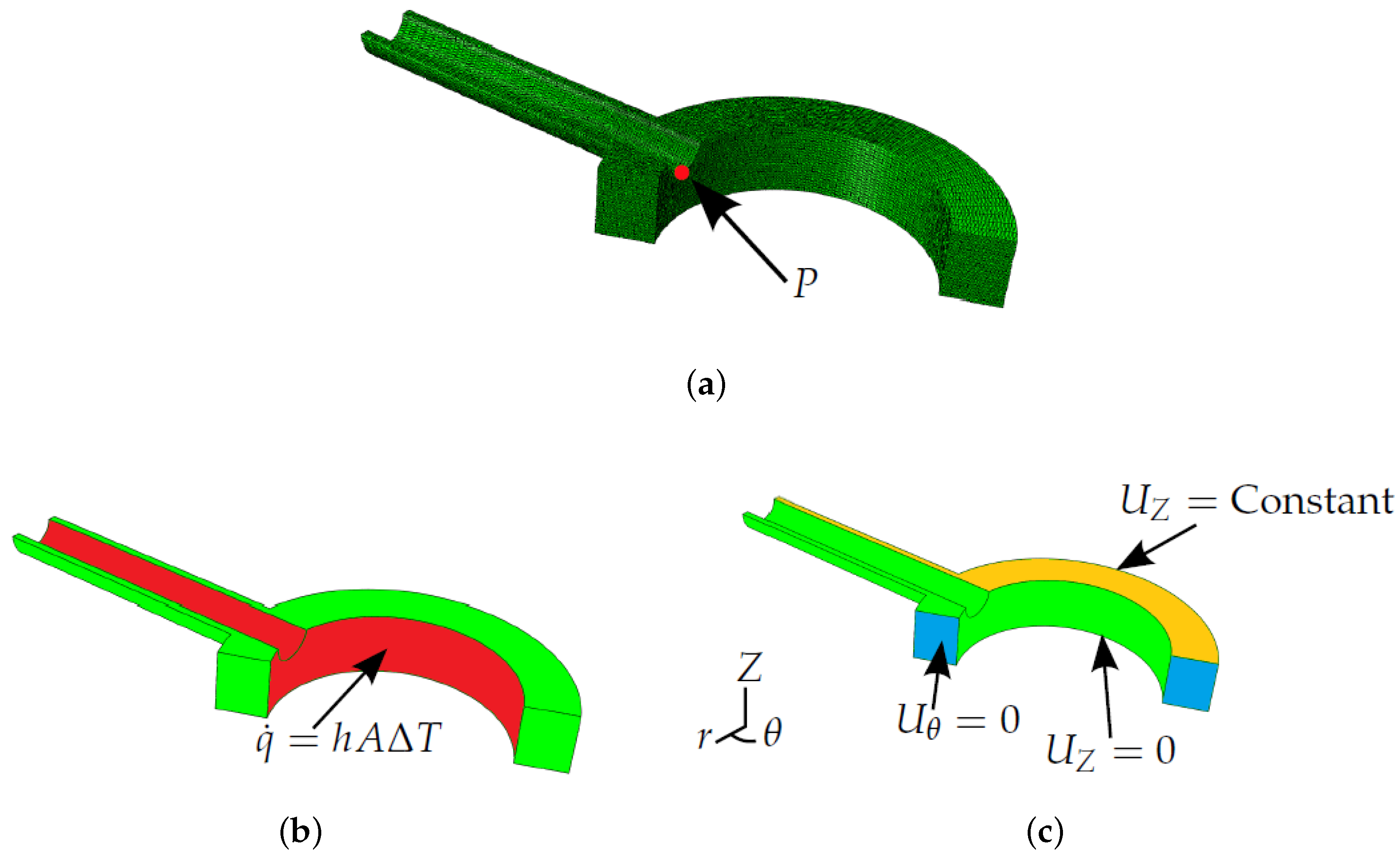
FEA models must be generated in order to determine the coefficients in Equation (10) and, thus, to define Green’s functions. FEA has been conducted in the present work using the commercially-available code ABAQUS (Dassault Systèmes, Paris, France). Since the present work looks to establish a method to introduce temperature dependency in the Green’s function method, a simplified two-stub penetration model has been used by way of example (see
Figure 1a, noting the plane of symmetry assumed between stub penetrations). Despite the simplified geometry, shell and stub dimensions are similar to those found in industry for P91 header components. Uncoupled thermoelastic analysis was conducted by first determining a temperature field from a heat transfer simulation. An insulated exterior boundary condition was assumed (
) to allow temperature fields in the model to reach equilibrium after the bulk steam temperature experiences a step change. Heat conduction on the inside surface of the header is controlled by convection (see
Figure 1b), where the heat transfer coefficient
h is taken to be a temperature-independent constant 0.002 W/mm
K. Once the transient temperature field has been determined, it can be used as an input in mechanical analyses to estimate thermal stress histories. Boundary conditions for the mechanical analysis can be seen in
Figure 1c. An “equation” type constraint [
19] is applied to the upper surface of the model (designated by the label
in
Figure 1c). This enforces equal displacements in the
Z direction between all nodes on this plane, thus ensuring it remains planar, and the assumed symmetry holds. Tetrahedral quadratic elements where used, namely DC3D10 (ABAQUS) for thermal analyses and C3D10 (ABAQUS) for mechanical analyses (see
Figure 1a for an example mesh) [
19]. In has been indicated in the literature that ligament cracking is a potential concern for header components, notably when thermal fatigue is a significant damage mechanism [
20]. As discussed previously, the Green’s function method allows for estimation of stresses at a singular analysis point only. With these factors in mind and for the illustration of the stress analysis potential of the Green’s function method, an analysis point (
P; see
Figure 1a) is considered in the present work that represents crack initiation at the inner bore [
20].
Figure 1.
Finite element analysis (FEA) models, showing: (a) the tetrahedral mesh, exploiting the plane of symmetry between stub penetrations and showing the location of the example point of interest P; (b) boundary conditions in the thermal analyses; and (c) boundary conditions in the mechanical analyses.
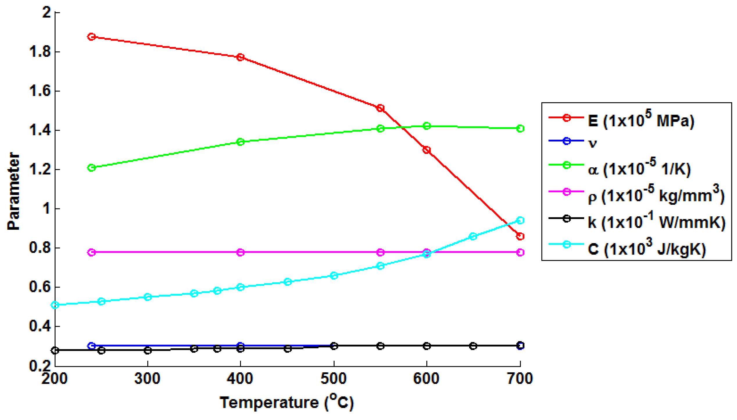
A single material is assumed for the FEA model in the present work (variations in material properties at the stub weld are not considered). Temperature-dependent material parameters are required in order to calculate transient thermal stresses within the header models. Values for Young’s modulus (
E) and the instantaneous thermal expansion coefficient (
α) have been determined from monotonic tests performed on an Instron 8862 thermomechanical fatigue machine (operating under isothermal conditions, Norwood, MA, USA) utilising radio frequency induction heating and using a TA instruments Q400 thermomechanical analyser (New Castle, DE, USA), respectively (see
Table 1). Tested temperature ranges were chosen to represent the typical bounds of operation for thermal power plant components. The remainder of the material constants have been taken from the work of Yaghi
et al. [
21] (
Table 2). A negligible dependency is assumed in density (
ρ) and Poisson’s ratio (
ν) over the tested temperature range. As such, values for these quantities are taken to be 7.76 ×
kg/mm
and 0.3, respectively. Temperature dependent material properties are summarised in
Figure 2.
Table 1.
A summary of the temperature-dependent material parameters (representative of a P91 chrome steel), determined through experimental analysis, used in the FEA modelling.
Table 1.
A summary of the temperature-dependent material parameters (representative of a P91 chrome steel), determined through experimental analysis, used in the FEA modelling.
| Temperature (℃) | Young’s Modulus (E) (N/mm) | Thermal Expansion Coefficient (α) () |
|---|
| 240 | 1.88 × | 1.21 × |
| 400 | 1.77 × | 1.34 × |
| 550 | 1.51 × | 1.41 × |
| 600 | 1.30 × | 1.42 × |
| 700 | 8.58 × | 1.41 × |
Table 2.
A summary of the temperature-dependent material constants (representative of a P91 chrome steel), taken from the work of Yaghi
et al. [
21], used in the FEA modelling.
Table 2.
A summary of the temperature-dependent material constants (representative of a P91 chrome steel), taken from the work of Yaghi et al. [21], used in the FEA modelling.
| Temperature (℃) | Thermal Conductivity (k) (W/mm.K) | Specific Heat Capacity (C) (J/kg.K) |
|---|
| 200 | 0.028 | 510 |
| 250 | 0.028 | 530 |
| 300 | 0.028 | 550 |
| 350 | 0.029 | 570 |
| 375 | 0.029 | 585 |
| 400 | 0.029 | 600 |
| 450 | 0.029 | 630 |
| 500 | 0.03 | 660 |
| 550 | 0.03 | 710 |
| 600 | 0.03 | 770 |
| 650 | 0.03 | 860 |
| 700 | 0.0305 | 942 |
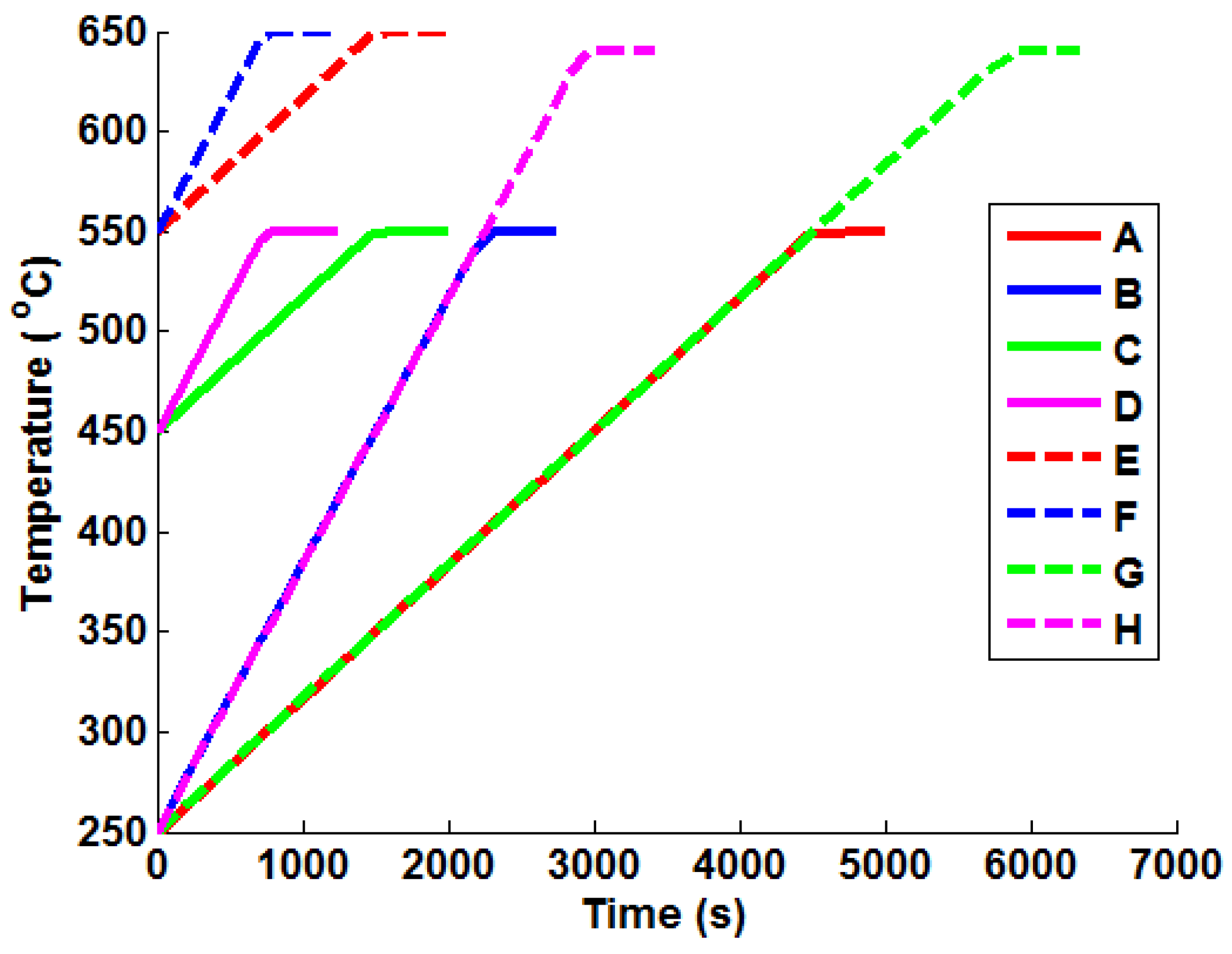
In order to apply the Green’s function method and the temperature interpolation techniques, realistic thermal stress histories must be generated from the FEA models for representative bulk steam temperature profiles (mechanical loading is neglected here, as it is a trivial exercise to scale linear elastic loads based on varying internal pressures). Several “ramp up” temperature profiles have been generated and analysed using the uncoupled thermoelastic procedure (with temperature-dependent material parameters). These are summarised in
Table 3 and are representative of the high end limiting bulk steam temperature increments and rates seen in two shifting plant. Plots of the ramp up temperature profiles can be seen in
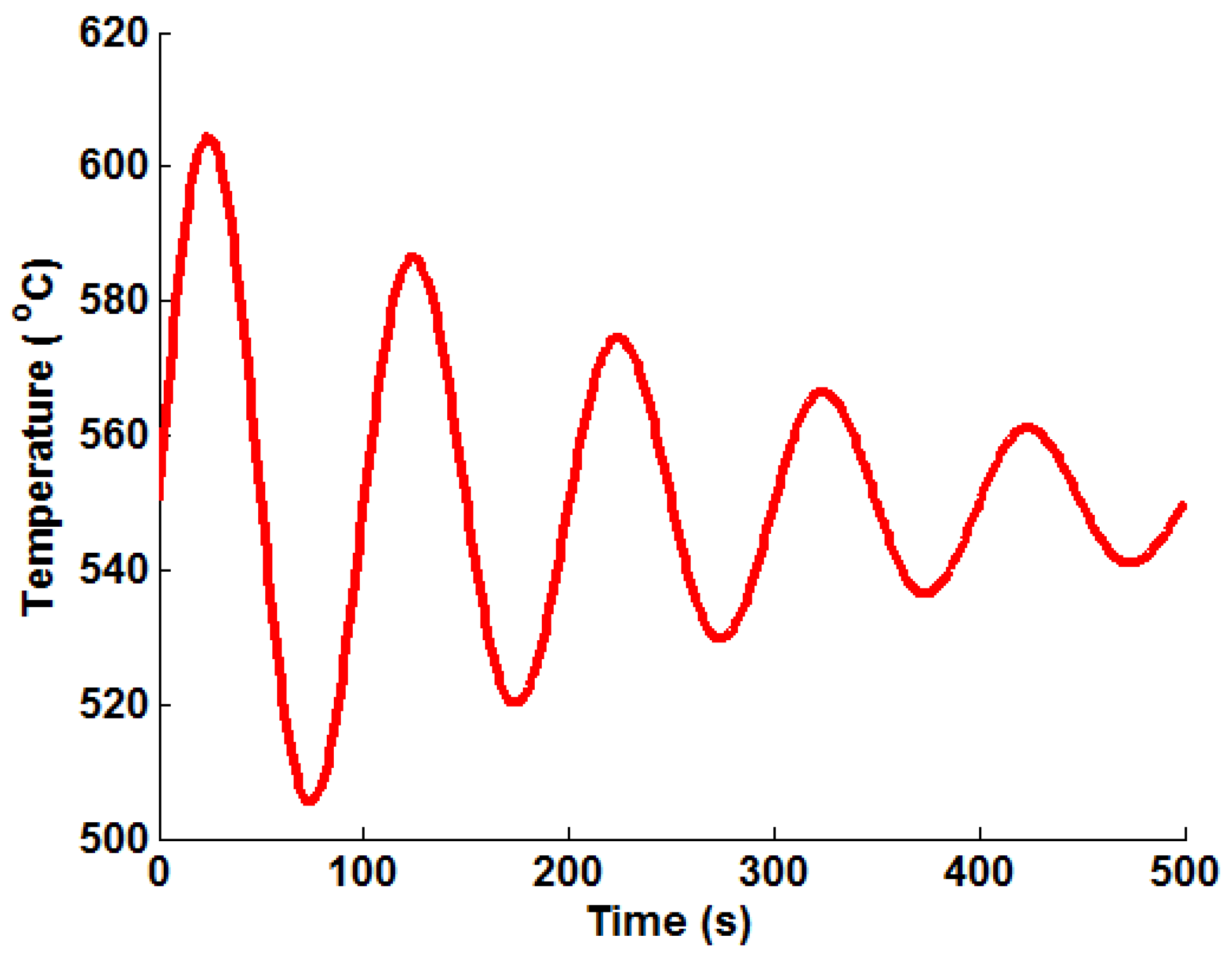
Figure 3 with their respective labels (which are used in the remainder of the present work). An oscillating temperature profile (that represents a control signal correcting bulk steam temperature to a nominal operating temperature of 550 ℃) is also considered (see
Figure 4), designated Profile “I”. This profile was generated using Equation (13), using the parameters
,
×
,
and
℃.
Figure 2.
A summary of the temperature-dependent material properties used in the present work to represent a P91 chrome steel.
Figure 2.
A summary of the temperature-dependent material properties used in the present work to represent a P91 chrome steel.
Table 3.
A summary of bulk steam temperature “ramp up” profiles.
Table 3.
A summary of bulk steam temperature “ramp up” profiles.
| Load Case | Start Temperature (℃) | End Temperature (℃) | Temperature Rate (℃/min) |
|---|
| A | 250 | 550 | 4 |
| B | 250 | 550 | 8 |
| C | 450 | 550 | 4 |
| D | 450 | 550 | 8 |
| E | 550 | 650 | 4 |
| F | 550 | 650 | 8 |
| G | 250 | 640 | 4 |
| H | 250 | 640 | 8 |
Figure 3.
Plots of the representative ramp up temperature profiles used to test the various Green’s function implementation techniques.
Figure 3.
Plots of the representative ramp up temperature profiles used to test the various Green’s function implementation techniques.
Figure 4.
A plot of the representative oscillating (decay) temperature profile used to test the various Green’s function implementation techniques.
Figure 4.
A plot of the representative oscillating (decay) temperature profile used to test the various Green’s function implementation techniques.
4. Methodology Overview
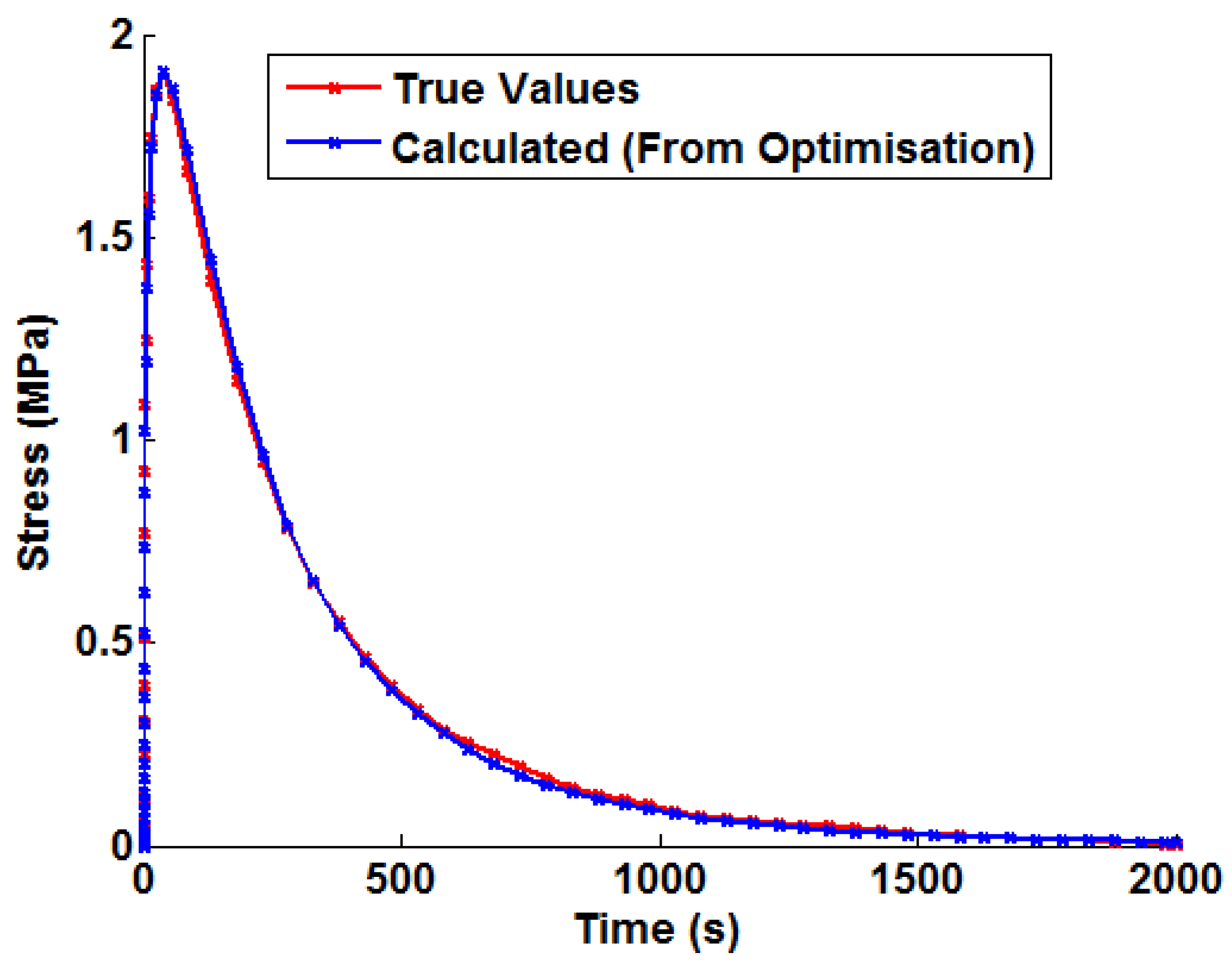
Prior to discussing the proposed method to introduce temperature dependency, it is worthwhile briefly discussing the procedure to determine temperature-independent Green’s functions. Once the thermally-driven stress profile has been determined from FEA for a unit bulk steam temperature step, the Green’s function approximation shown in Equation (10) can by fitted (an example may be seen in
Figure 5). This defines the constants
,
. A non-linear least squares optimisation algorithm (the Levenberg—Marquardt algorithm) was used in a MATLAB program (function LSQNONLIN [
22], MathWorks, Natick, MA, USA) to optimise the values of Equation (10) in order to fit the FEA solution.
Figure 5.
An example of the Green’s function approximation (shown in Equation (10)) fitted to the von Mises stress history from an uncoupled thermoelastic FEA simulation (unit temperature step).
Figure 5.
An example of the Green’s function approximation (shown in Equation (10)) fitted to the von Mises stress history from an uncoupled thermoelastic FEA simulation (unit temperature step).
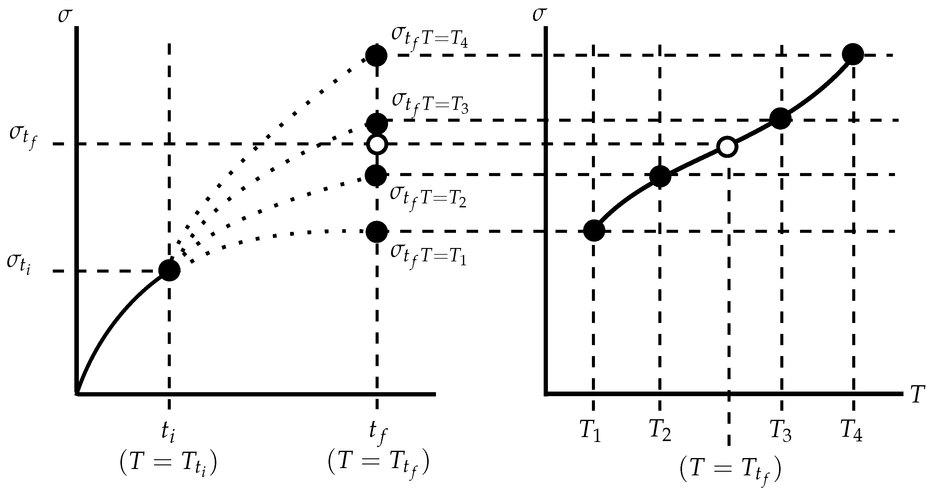
A schematic of the proposed interpolation technique is given in
Figure 6. The Green’s function method fundamentally relies on determining a reference solution for a unit temperature step that may be integrated for a particular thermal loading history. By including temperature dependency, this reference solution will need to be altered over the thermal history. The proposed technique achieves this by interpolating between solutions determined from temperature-independent Green’s functions. Green’s functions are determined for unit temperature steps, each of which has an associated representative temperature (taken here to be the mean temperature for the unit step). Given some initial conditions (
σ =
,
T =
), stress increments can be determined for each Green’s function (
,
, and so on, with the representative temperatures
; see Equation (14)). Note that a different (temperature dependent) set of constants (
) is used to find each reference solution (
). These constant sets are designated
for representative temperatures
, respectively, in Equation (14). The relationship between the representative temperatures and reference stress values may then be used to interpolate to the actual instantaneous temperature
and, thus, find the estimated stress increment
. A suitably high order polynomial may be used to model this relationship. For
M reference solutions and representative temperatures, Equation (15) may be used, where
are the coefficients of the polynomial. Generating the reference curves in this way allows the relationship between stress values predicted by particular Green’s functions at a time instant to change with time, thus allowing the second order effect (
) to be accounted for.
Figure 6.
A schematic of the proposed interpolation technique.
Figure 6.
A schematic of the proposed interpolation technique.
6. Discussion and Conclusions
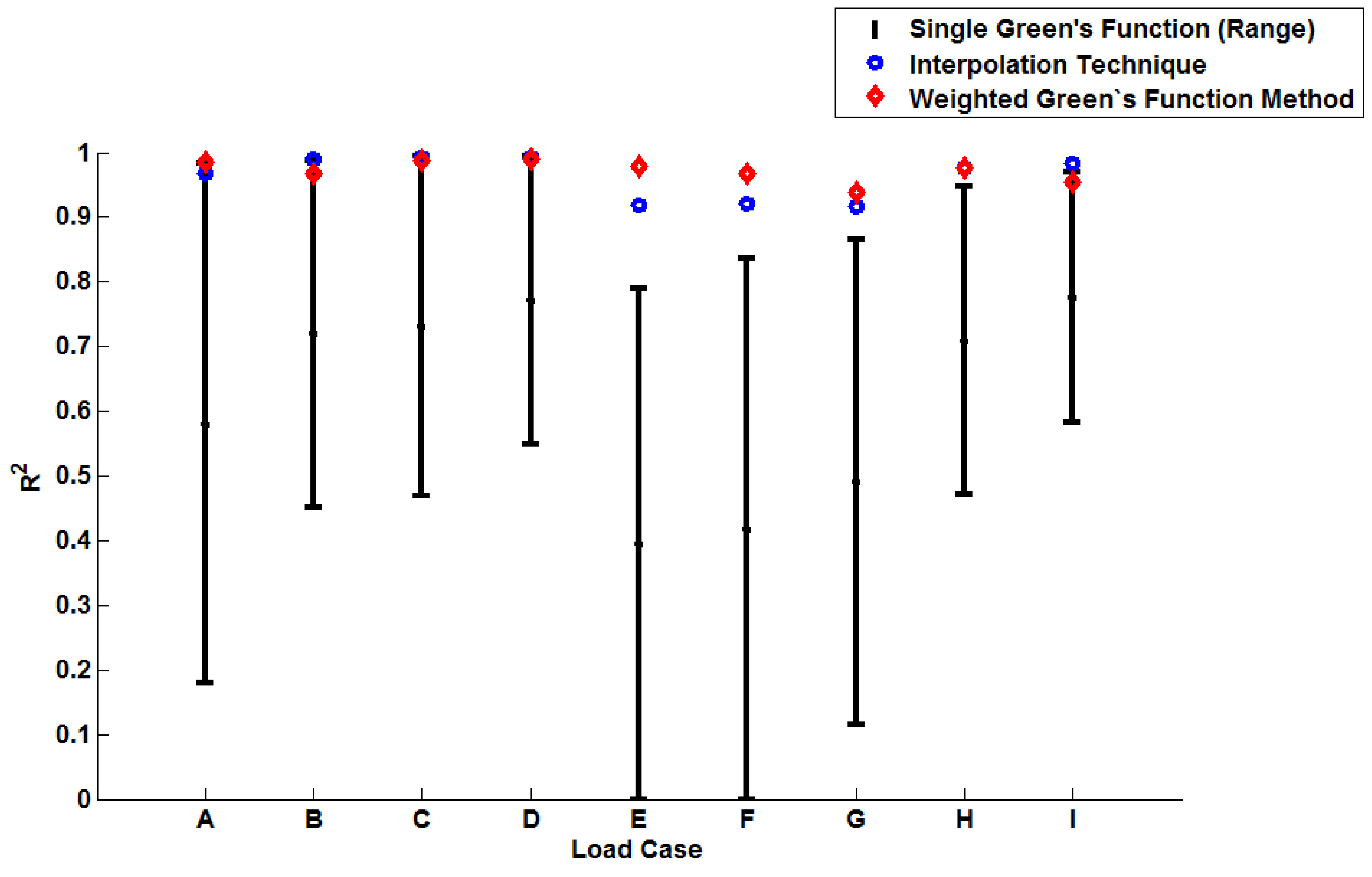
The coefficient of determination (
) provides a statistical measure to describe the amount of variance accounted for in a model when predicting some “true” data (taking limiting values of zero if no variance is accounted for and one if all variance is accounted for [
23]). The values determined for
shown in
Table 6 are plotted in
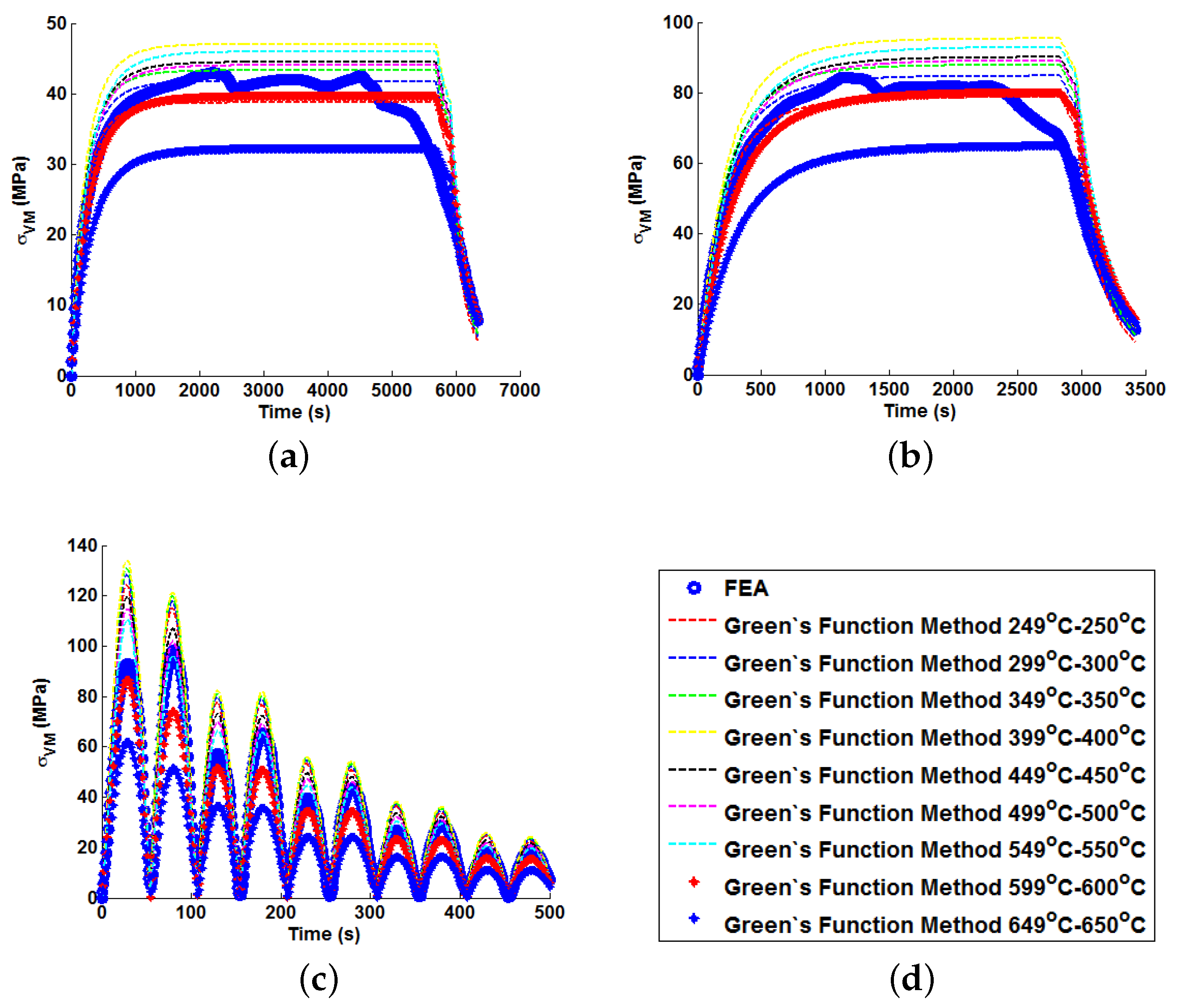
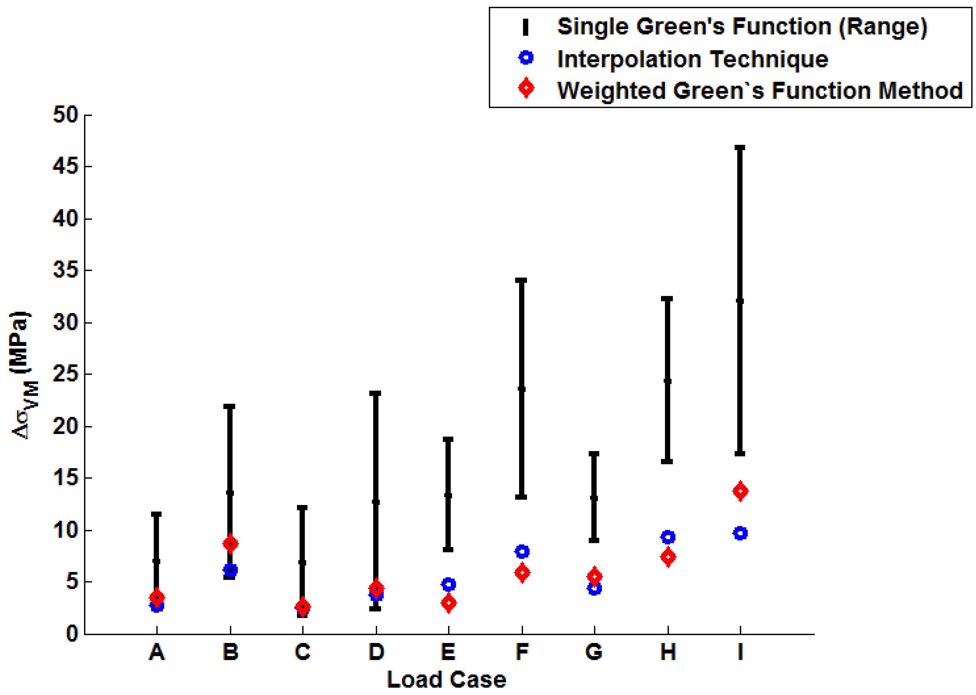
Figure 14 (note the range of values determined when using individual Green’s functions is presented). Similarly, a plot of the peak instantaneous stress differences (
; see
Table 7) is given in
Figure 15. This quantity is of interest as, when attempting to quantify the threat of thermal fatigue using a reference elastic solution, stress ranges experienced in a component are one of the most fundamental ways to characterise a particular loading scenario.
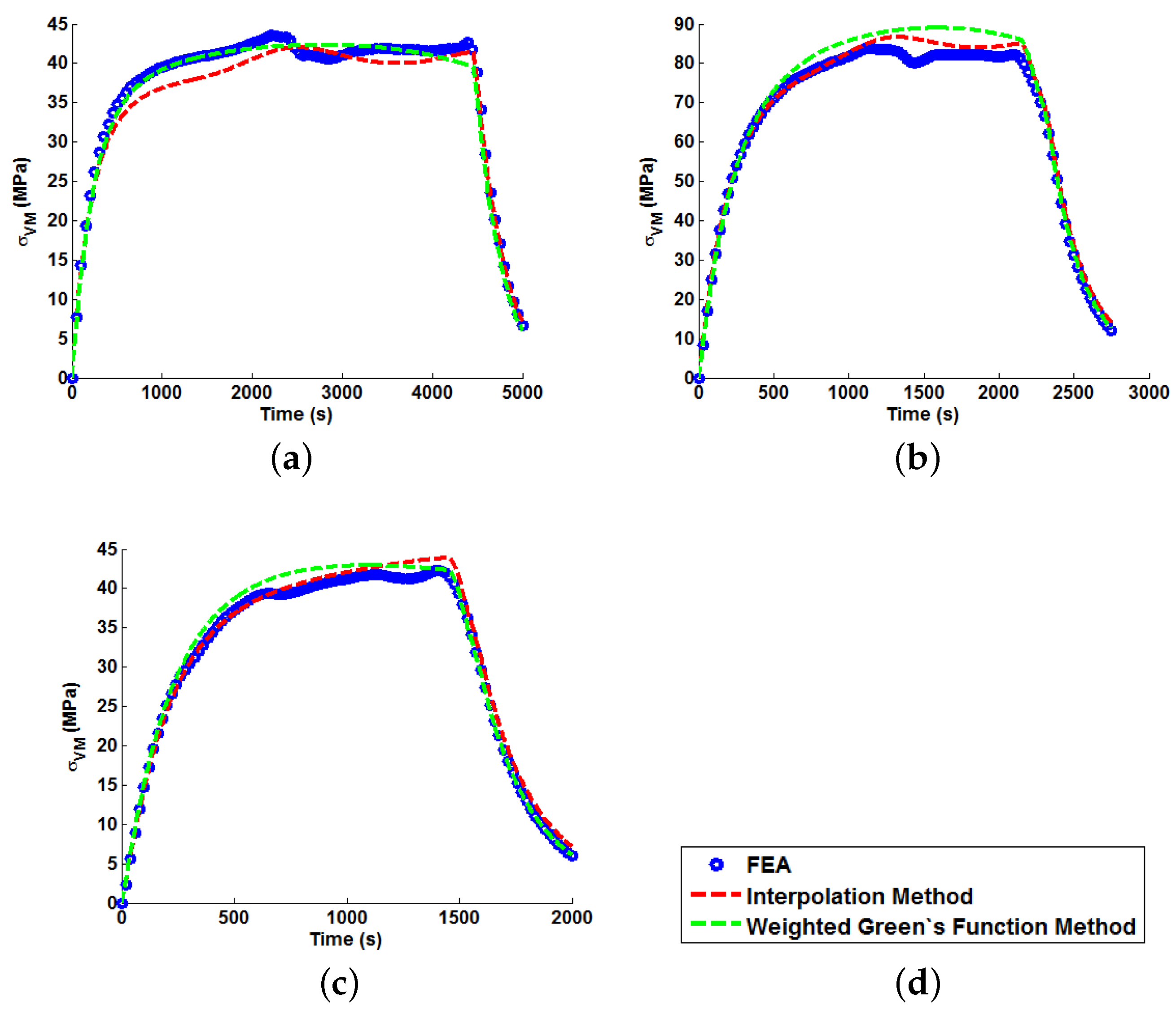
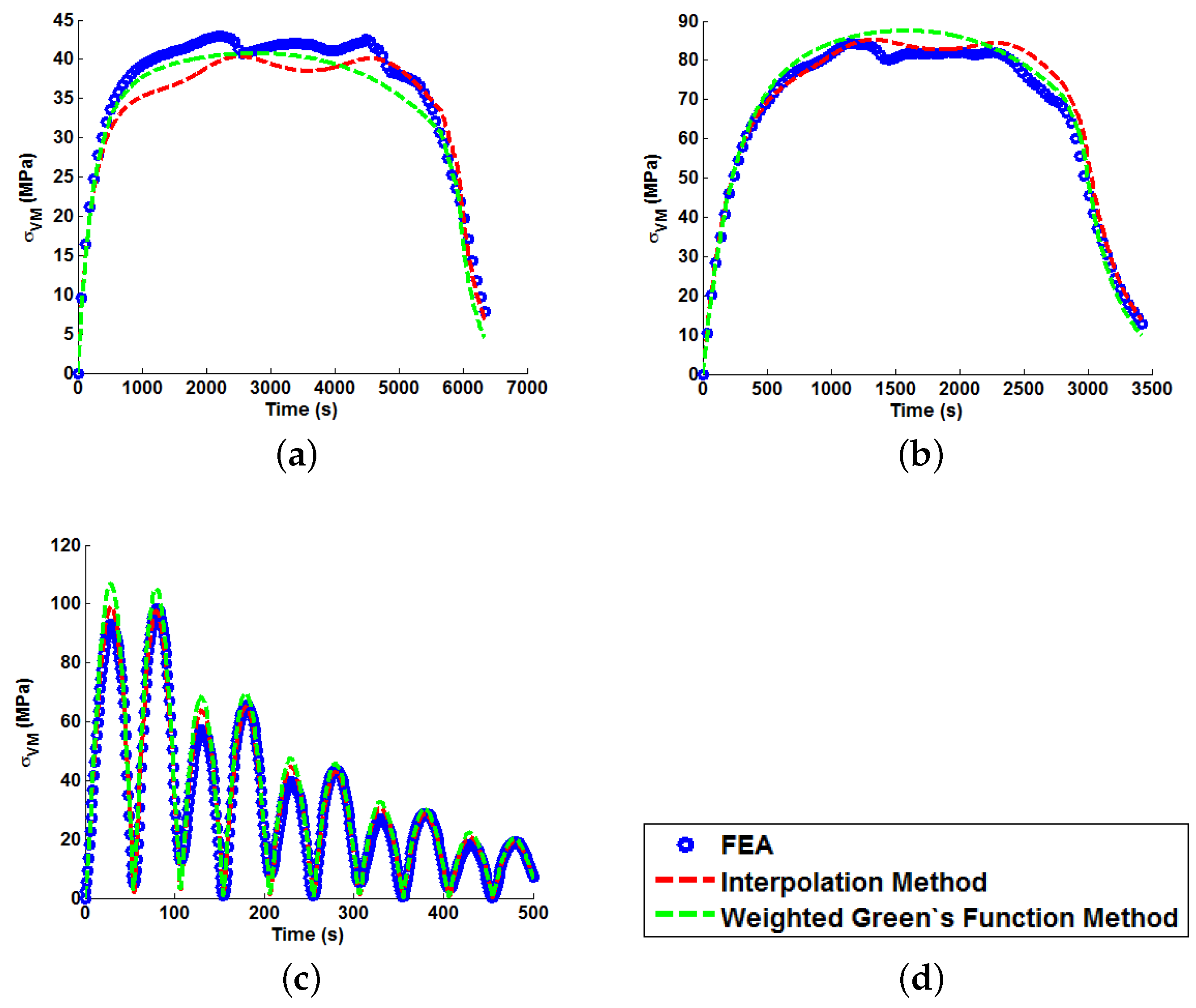
In all cases, solutions where temperature dependency was considered in the Green’s function method showed an improvement in fitting quality. All results were at least in the 98th percentile of the range predicted when using individual Green’s functions (for the majority of cases,
and
values were better than even the optimum individual Green’s function solution). Despite the small number of load cases considered, some general comments can be made.
values are comparable for most cases, and in almost all cases, the interpolation technique resulted in lower
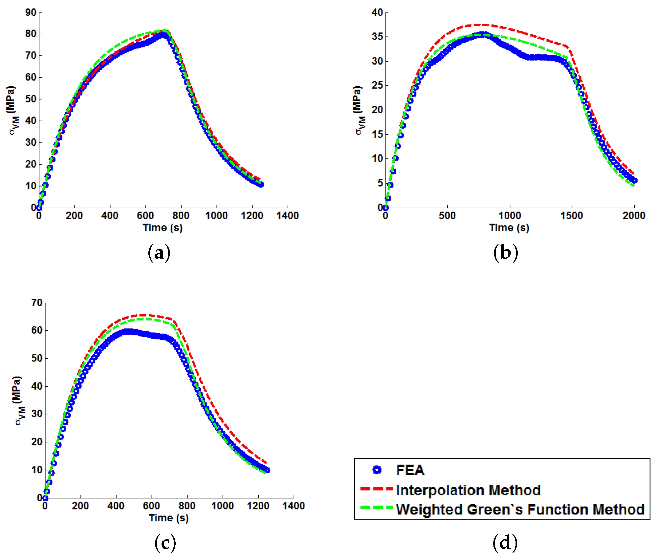
values than the weighting function technique (suggesting small stress over-/under-estimations). Anomalies to these observations are found in load Cases E and F, where the weighting function method appears to give superior results, represented by an approximate 2 MPa reduction in stress differences. It is also noted from
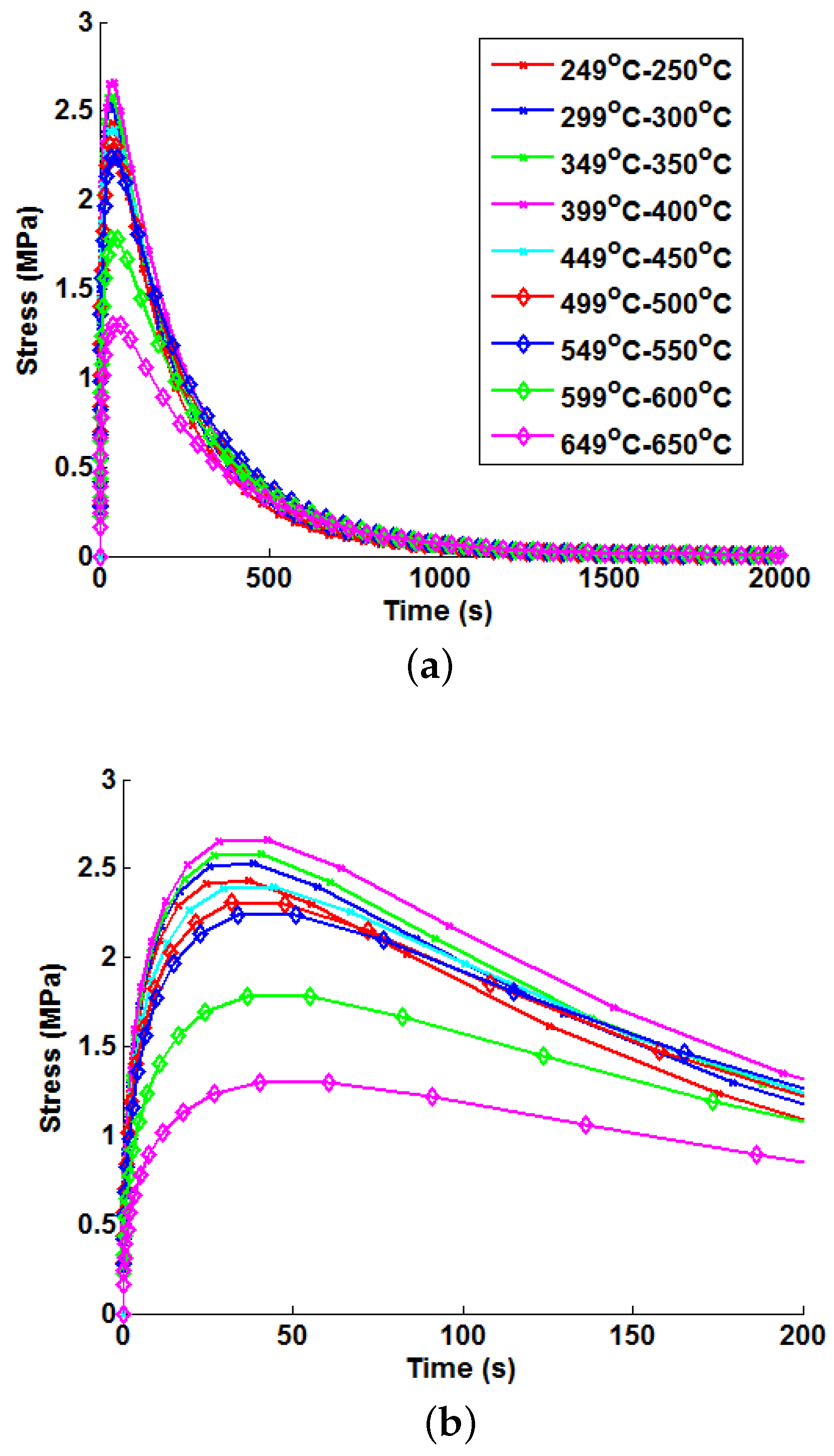
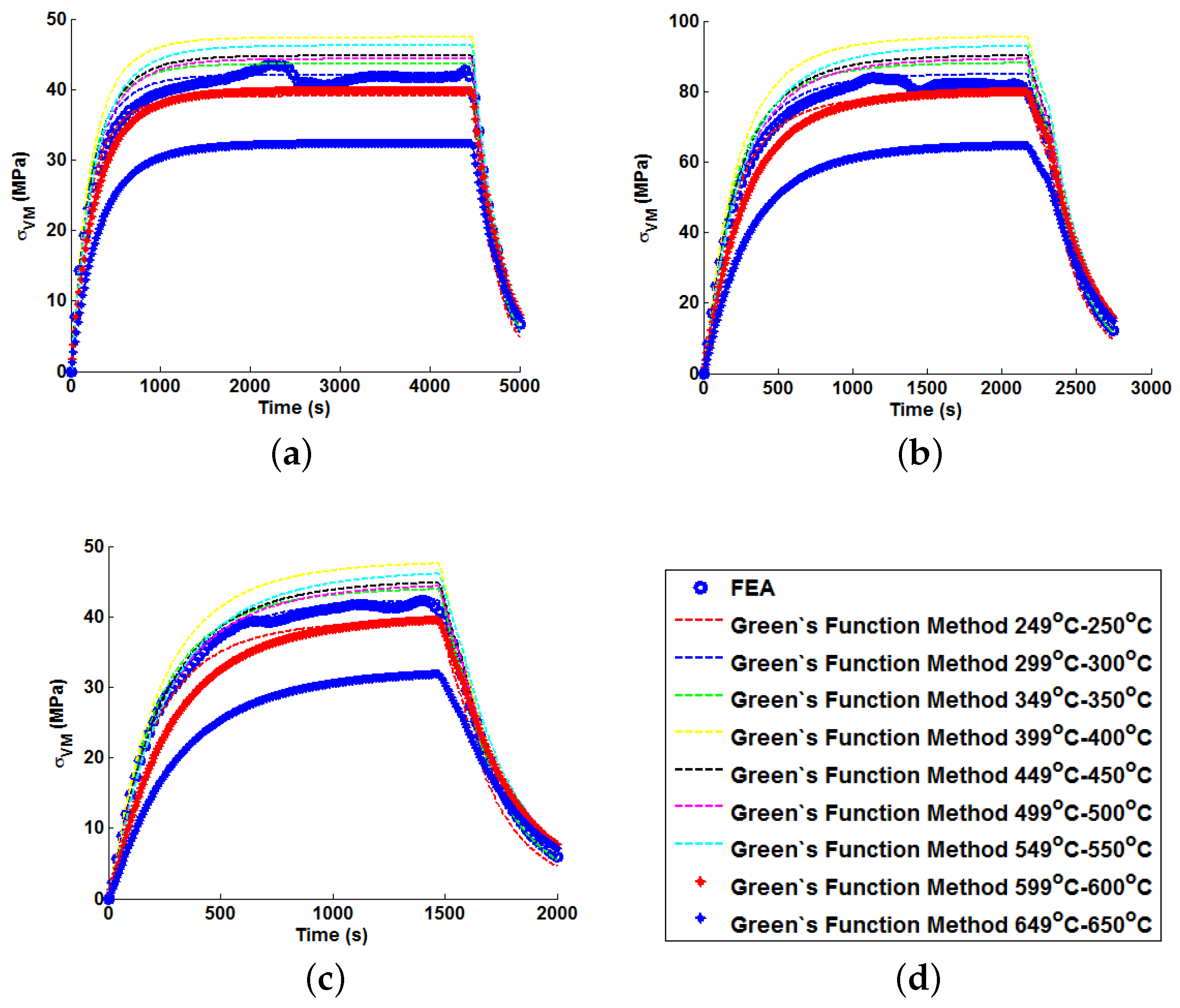
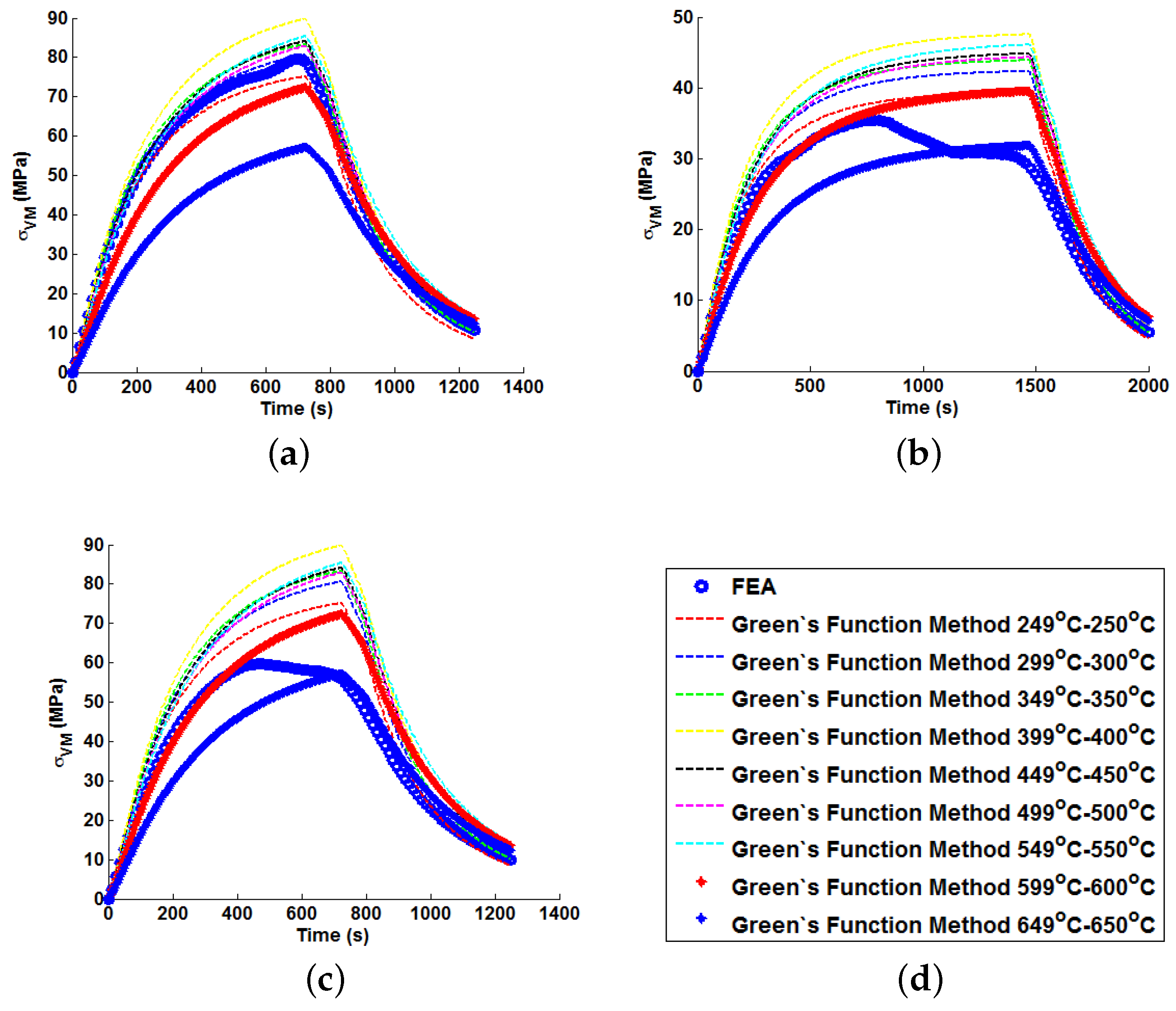
Figure 11,
Figure 12 and
Figure 13 that load cases with large temperature increments (Cases A, B, G and H) do not result in smooth stress development curves that monotonically increase to a maximum value and then decay (
i.e., there are “ripples” in the thermal stress histories; see
Figure 11b in particular). These features are not seen in more modest temperature step load cases.
Figure 14.
A plot to show the relative performance of the various implementation methods (using ).
Figure 14.
A plot to show the relative performance of the various implementation methods (using ).
Figure 15.
A plot to show the relative performance of the various implementation methods (using ).
Figure 15.
A plot to show the relative performance of the various implementation methods (using ).
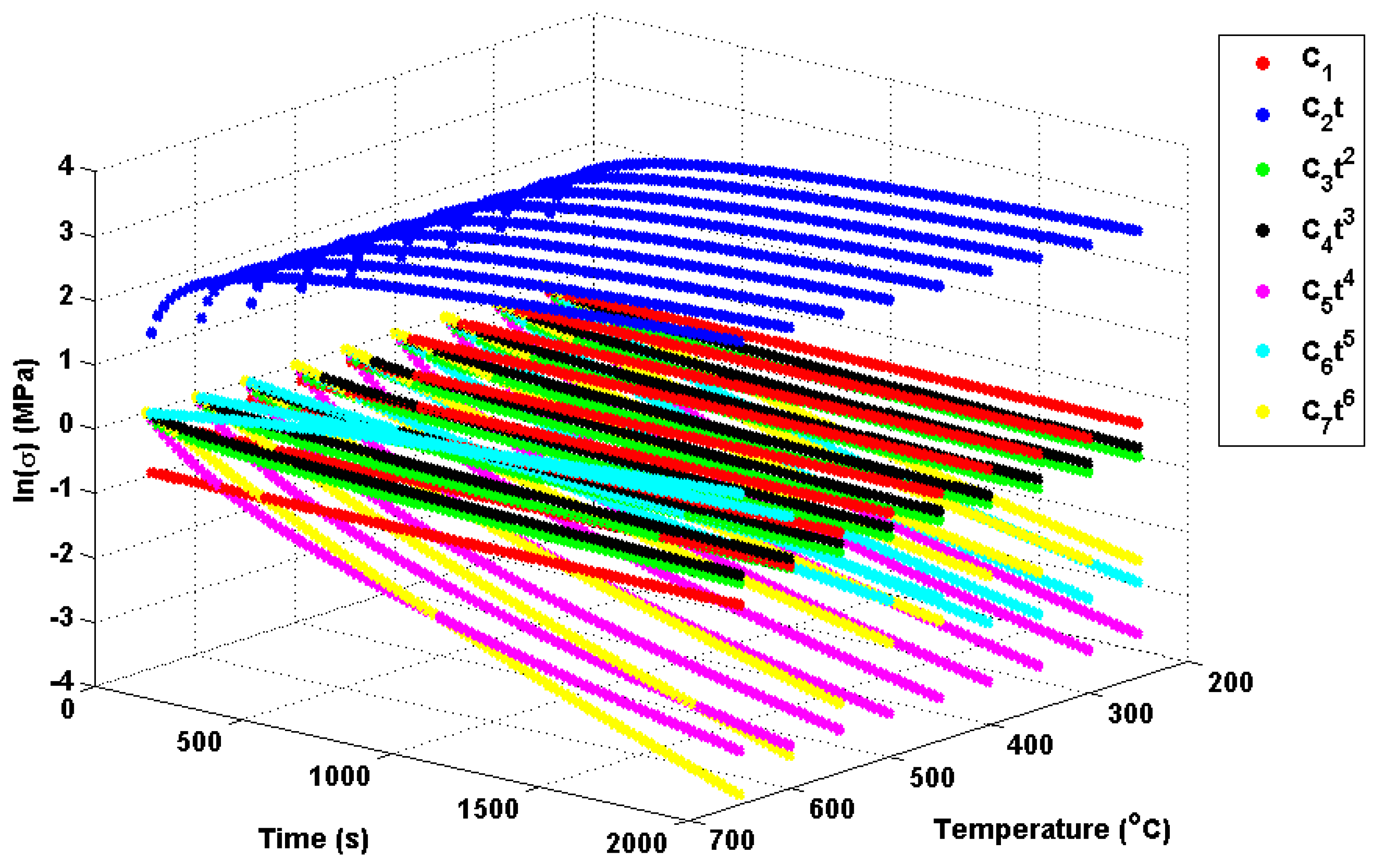
Potential explanations for these behaviours can be found from analysis of the individual Green’s function components themselves and, in particular, the relative effects of the seven exponential components. These components are plotted in
Figure 16 using the Green’s function coefficients given in
Table 4. Of interest for the present work are the fifth and sixth order components (the
and
terms, respectively; most other components vary little over the given temperature range), which can be seen to (in part) control stress decay in the unit Green’s functions. Furthermore, there is a shift at around 450 ℃, with the sixth order component becoming more dominant in the decay characteristics and the fifth order component becoming positive (leading to a small contribution in stress development). Over large temperature ranges, multiple Green’s functions may be used with a wide range of decay characteristics. The “ripple” features discussed previously are therefore due to the complex (time dependent) interaction of these decay functions. While varying decay characteristics can be accounted for in the proposed interpolation method, the time-independent weight function assumes a scaling dependent only on temperature (hence, the superior fit observed for the interpolation method in Cases A, B, G and H). Cases C–F used temperature ranges between 450 and 650 ℃, where the relationship between components in Green’s function is reasonably linear (with temperature) and can therefore be accounted for using the weighting function. As the weighting function coefficients are estimated by an optimisation procedure using all unit responses, this linear relationship can be approximated, and local errors in the (particularly in the 450 ℃ and 650 ℃ profiles) can be minimised.
The proposed interpolation method has been shown to be adept at predicting thermal stress histories in thick-walled components. Over large temperature ranges (>150 ℃), where material properties may vary significantly, the interpolation procedure has out performed the weighting method. For more modest temperature ranges, the two methods are generally comparable. In addition to the increased generality that the interpolation procedure offers, it is worth highlighting important practical advantages. The order of the weighting function polynomial given in Equation (12) is ultimately dependent on the number of reference solutions generated. In the present work, nine unit temperature steps were applied to FEA models and used in the temperature dependency methods. Fewer reference solutions may be used in practice, however, due to practical limitations, potentially limiting the applicability of the weighting function. While a greater number of reference solutions is beneficial to the interpolation procedure, even a small number can be used to understand core variations in stress profiles with representative temperature. Some aspects of the second order effects may therefore also be captured. Future work will look to quantify the effect the number of available reference solutions has on the performance of the temperature dependency methods.
In conclusion, the present work has highlighted the importance of including temperature dependency in the Green’s function method in order to better estimate transient thermal stresses for realistic bulk steam temperature increments in thick-walled components. The proposed interpolation technique provides a general procedure to incorporate temperature dependency in Green’s function analysis. There is some suggestion from the results that the relative importance of each Green’s function component varies with temperature and leads to complex interactions between thermal stress development and decay terms. Over larger temperature ranges, this has been seen to have an effect; however, for small temperature ranges, the weighting function method proposed by Koo
et al. appears to be satisfactory [
17]. Future work will therefore focus on increasing the number of load cases considered in order to verify the suggested phenomenon and in accounting for spatial variations in material properties and chosen analysis points.
Figure 16.
Decomposed Green’s functions, showing the relative importance of the exponential components.
Figure 16.
Decomposed Green’s functions, showing the relative importance of the exponential components.


