A Theory of Elastic/Plastic Plane Strain Pure Bending of FGM Sheets at Large Strain


1
School of Mechanical Engineering and Automation, Beihang University, No. 37 Xueyuan Road, Beijing 100191, China
2
Ishlinsky Institute for Problems in Mechanics, 101-1 Prospect Vernadskogo, 119526 Moscow, Russia
3
Department of Civil Engineering, National Cheng Kung University, 1 University Road, Tainan 70101, Taiwan
*
Author to whom correspondence should be addressed.
Materials 2019, 12(3), 456; https://doi.org/10.3390/ma12030456
Submission received: 31 December 2018
/
Revised: 24 January 2019
/
Accepted: 28 January 2019
/
Published: 1 February 2019
(This article belongs to the Special Issue Advances in Mechanical Problems of Functionally Graded Materials and Structures)
Abstract
:An efficient analytical/numerical method has been developed and programmed to predict the distribution of residual stresses and springback in plane strain pure bending of functionally graded sheets at large strain, followed by unloading. The solution is facilitated by using a Lagrangian coordinate system. The study is concentrated on a power law through thickness distribution of material properties. However, the general method can be used in conjunction with any other through thickness distributions assuming that plastic yielding initiates at one of the surfaces of the sheet. Effects of material properties on the distribution of residual stresses are investigated.
1. Introduction
Structures made of functionally graded materials (FGM) are advantageous for many applications. A difficulty with theoretical analysis and design is that structures made of FGM are classified by a much greater number of parameters than similar structures made of homogeneous materials. For this reason, it is desirable to perform parametric studies by analytic or semi-analytic methods as much as possible. A review of results related to the analysis of FGM and published before 2007 is presented in [1]. This review focuses on structures with through-thickness variation of material properties. Analytic solutions derived in [1,2,3,4,5] belong to this class of FGM as well. In [2,3,4], elastic and elastic/plastic spherical vessels subjected to various loading conditions are considered. Thermo-elastic simply supported and clamped circular plates are studied in [5]. Many analytic and semi-analytic solutions are available for FGM discs and cylinders assuming that material properties vary in the radial direction but are independent of the circumferential and axial directions. Purely elastic solutions for a hollow disc or cylinder subjected to internal or/and external pressure are derived in [6,7,8]. An axisymmetric thermo-elastic solution for a hollow cylinder subjected quite a general system of thermo-mechanical loading is presented in [9]. It is assumed that the temperature varies along the radial coordinate. A plane strain analytic elastic/plastic solution for pressurized tubes is found in [10]. The solution is based on the Tresca yield criterion. Many solutions are proposed for functionally graded solid and hollow rotating discs. Purely elastic solutions for solid discs of constant thickness are given in [11,12], a purely elastic solution for a hollow disc of variable thickness in [13], a purely elastic solution for hollow polar orthotropic discs in [14], and a solution for hollow cylinders using the theory of electrothermoelasticity in [15]. An elastic perfectly plastic stress solution for hollow discs is derived in [16] using the von Mises yield criterion.
All of the aforementioned solutions deal with infinitesimal strain. A distinguished feature of the solution provided in the present paper is that strains are large. The process considered is pure bending of a FGM sheet under plane strain conditions. A review on bending of functionally graded sheets and beams at infinitesimal strains is given in [17]. The present solution is based on the approach proposed in [18]. It is shown in this paper that the use of Lagrangian coordinates facilitates the solution. Moreover, the equations describing kinematics can be solved independently of stress equations in the case of isotropic incompressible material. This is an advantage as compared to the classic approach developed in [19] where the stress equations are solved first. The classic approach is restricted to perfectly plastic materials, whereas the mapping in Equation (1) is valid for a large class of constitutive equations. The approach proposed in [18] has already been successfully extended to more general constitutive equations in [20,21,22,23]. It is shown in the present paper that the approach is also efficient for FGM sheets. It is worth noting that a rigid plastic solution for pure bending of laminated sheets (such sheets can also be referred to as functionally graded sheets) at large strain is given in [24].
2. Basic Equations
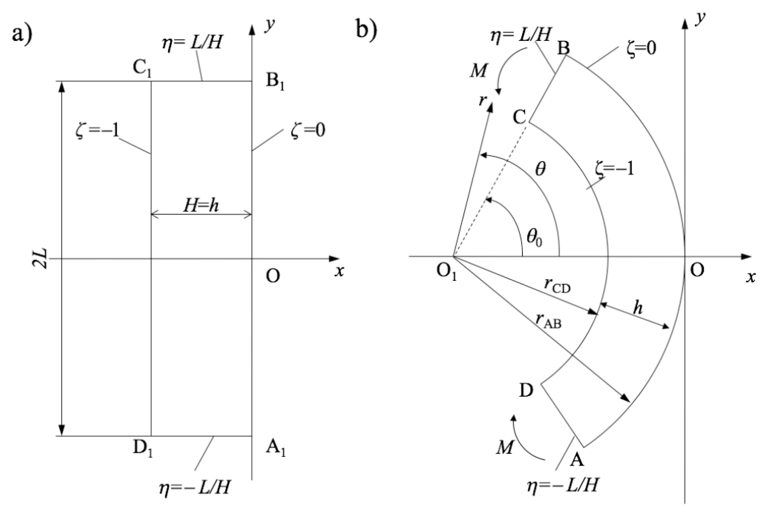
The process of plane strain pure bending is illustrated in Figure 1. The approach proposed in [18] for solving the corresponding boundary value problem is based on the following transformation equations:
where is an Eulerian–Cartesian coordinate system and is a Lagrangian coordinate system. Without loss of generality, it is possible to assume that the origin of the Cartesian coordinate system is located at the intersection of the axis of symmetry of the process and the outer surface and that the x-axis coincides with the axis of symmetry. The Lagrangian coordinate system is chosen such that
at the initial instant where H is the initial thickness of the sheet. It is evident from these relations and the geometry in Figure 1 that on AB, on CD, on CB and on AD throughout the process of deformation. Here, L is the initial width of the sheet. In Equation (1), a is a time-like variable. In particular, at the initial instant. In Equation (1), s is a function of a. This function should be found from the stress solution and therefore depends on constitutive equations. The condition in Equation (2) is satisfied if
at . It is possible to verify by inspection that the mapping in Equation (1) satisfies the equation of incompressibility. Moreover, this mapping transforms initially straight lines and into circular arcs AB and CD and initially straight lines and into circular arcs CB and AD after any amount of deformation (Figure 1). Furthermore, coordinate curves of the Lagrangian coordinate system coincide with trajectories of the principal strain rates and, for coaxial models, with trajectories of the principal stresses. Thus, the shear stress vanishes in the Lagrangian coordinates. In particular, the contour ABCD is free of shear stresses. Let and be the physical stress components referred to the Lagrangian coordinates. The stress solution should satisfy the boundary conditions
for and . The only non-trivial equilibrium equation in the Lagrangian coordinates has been derived in [18] as
The initial plane strain yield criterion of the functionally graded sheet is supposed to be
where is a material constant and is an arbitrary function of its argument. It is assumed that material properties are not affected by plastic deformation. Therefore, Equation (6) can be rewritten in the form
In this case, the yield locus is invariant along the motion. The importance of this property of material models has been emphasized in [25]. Let and be the deviatoric portions of and , respectively. Since the material is incompressible, under plane strain conditions. Then, the yield criterion in Equation (7) is equivalent to
Hooke’s law generalized on functionally graded materials reads
It has been taken into account here that Poisson’s ratio is equal to 1/2 for incompressible materials. In addition, and are the total strain components in elastic regions and the elastic portions of the total strain components in plastic regions referred to the Lagrangian coordinate system, is a material constant and is an arbitrary function of its argument.
3. Stress Solution at Loading
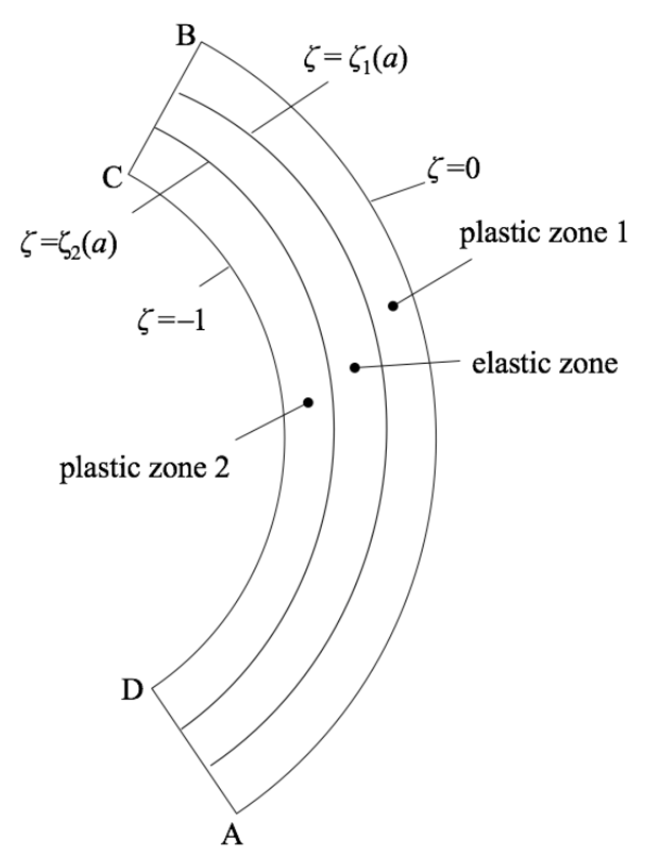
It is assumed that the functions and involved in Equations (7) and (9) are such that plastic yielding can only initiate at or . This assumption can be verified using the purely elastic solution with no difficulty. At the very beginning of the process, the entire sheet is elastic. As deformation proceeds, one of the following three cases arises: (i) plastic yielding initiates at the surface ; (ii) plastic yielding initiates at the surface ; and (iii) plastic yielding initiates simultaneously at the surfaces and . These cases should be treated separately. In the following, is the elastic/plastic boundary between the plastic region that propagates from the surface and the elastic region and is the elastic/plastic boundary between the plastic region that propagates from the surface and the elastic region. It is evident that both and depend on a. The general structure of the solution with two plastic regions is illustrated in Figure 2. Let M be the bending moment. Then, its dimensionless representation is in terms of the Lagrangian coordinates given by [18]
In the elastic region, the whole strain is elastic. Therefore, it follows from Equation (1) that the principal logarithmic strains are
Integrating this equation with respect to and using the boundary condition in Equation (4) at leads to
where and is a dummy variable of integration. The expression for in Equation (15) has been derived using the identity , and Equations (9) and (12). In the case of the purely elastic solution, Equation (15) must satisfy the boundary condition in Equation (4) at . Then, the equation for the function s(a) is
Using Equation (15), in which s should be eliminated by means of the solution of Equation (16), and the yield criterion in Equation (8), it is possible to determine which of the three cases mentioned above occurs for given material properties. Simultaneously, the value of a at which plastic yielding initiates is determined. This value of a is denoted as . In the following, it is assumed that . It is now necessary to consider Cases (i), (ii) and (iii) separately.
Case (i). There are two regions. A plastic region occupies the domain and an elastic region the domain . Equation (15) is valid in the elastic region. However, the function is not determined from Equation (16). It is reasonable to assume that in the plastic region. Therefore, the yield criterion in Equation (7) becomes
Substituting Equation (17) into Equation (5) and integrating yields the dependence of the stress on . Using Equation (17) again provides the dependence of the stress on . As a result,
It is evident that this solution satisfies the boundary condition in Equation (4) at . Both and should be continuous across . Consequently, is continuous across . The stress on the elastic side of the elastic/plastic boundary is determined from Equation (15) and on the plastic side from Equation (8). Then, the condition of continuity of across the surface is represented as
Solving this equation for s yields
Using Equations (15) and (18), the condition of continuity of across the surface is represented as
In this equation, s can be eliminated by means of Equation (20). The resulting equation should be solved numerically to find as a function of a. Then, s as a function of a is readily found from Equation (20). The yield criterion should be checked in the elastic region using the solution in Equation (15). The calculation should be stopped when the yield condition is satisfied at one point of the elastic region. Denote the corresponding value of a as .
In Case (i), Equation (11) becomes
In the first integrand, should be eliminated by means of Equation (18) and in the second by means of Equation (15).
Case (ii). There are two regions. A plastic region occupies the domain and an elastic region the domain . The elastic solution in Equation (15) satisfies the boundary condition in Equation (4) at . Therefore, it is convenient to rewrite this solution as
The elastic solution in this form satisfies the boundary condition in Equation (4) at . It is reasonable to assume that in the plastic region. Therefore, the yield criterion in Equation (7) becomes
Substituting Equation (24) into Equation (5) and integrating yields the dependence of the stress on . Using Equation (24) again provides the dependence of the stress on . As a result,
It is evident that this solution satisfies the boundary condition in Equation (4) at . Both and should be continuous across . Consequently, is continuous across . The stress on the elastic side of the elastic/plastic boundary is determined from Equation (23) and on the plastic side from Equation (8). Then, the condition of continuity of across the surface is represented as
Solving this equation for s yields
In this equation, s can be eliminated by means of Equation (27). The resulting equation should be solved numerically to find as a function of a. Then, s as a function of a is readily found from Equation (27). The yield criterion should be checked in the elastic region using the solution in Equation (23). The calculation should be stopped when the yield condition is satisfied at one point of the elastic region. Denote the corresponding value of a as .
In Case (ii), Equation (11) becomes
In the first integrand, should be eliminated by means of Equation (23) and in the second by means of Equation (25).
Case (iii). In this case, there are two plastic regions, and , and one elastic region, . At the beginning of this stage of the process, and or and . Let be the value of at and be the value of at . Then, the elastic solution in Equation (15) can be rewritten as
It follows from this solution that
The solution in Equation (18) is valid in the plastic region and the solution in Equation (25) in the plastic region . Then,
and
Eliminating in this equation s by means of Equation (20) or Equation (27) and then a by means of Equation (35) supplies the equation to find as a function of (or as a function of ). Then, a as a function of (or ) is found from Equation (35) and s as a function of (or ) from Equation (20) or (27). The distribution of the stresses is determined from Equation (30) with the use of Equations (32) and (33) in the elastic region, from Equation (18) in the region and from Equation (25) in the region .
In Case (iii), Equation (11) becomes
4. Unloading
It is assumed that unloading is purely elastic. This assumption should be verified a posteriori. At this stage of the process, the strains can be considered as infinitesimal. Let and be the values of a and s, respectively, at the end of loading. These values are known from the solution given in the previous section. Using Equation (10), the values of and at the end of loading, and , are determined as
It is convenient to introduce a polar coordinate system with the origin at and (point in Figure 1). The coordinate curves of this coordinate system coincide with the coordinate curves of the -coordinate system. Therefore, and where and are the normal stresses in the polar coordinate system. Moreover, at and at . The equilibrium equation for the increment of the stresses, and , in the polar coordinate system can be written as
where . Since at and at any stage of the process, the increment of this stress should satisfy the conditions
for and .
The displacement components from the configuration corresponding to the end of loading in the polar coordinate system are supposed to be
where and are dimensionless constants. Using Equation (41), the increment of the normal strains in the polar coordinate system is determined as
The increment of the deviatoric stresses is found from Equation (42) and the Hooke’s law (Equation (9)) where the stresses and strains should be replaced with the corresponding increments. Then,
Using this solution, the right hand side of Equation (36) can be rewritten as
The Lagrangian coordinate at the end of loading is expressed in terms of as [18]
Using this equation, it is possible to eliminate in Equation (44). Then, substituting Equation (44) into Equation (39) and integrating gives
It is evident that this solution satisfies the boundary condition in Equation (40) at (or ). The other boundary conditions in Equations (40) and (46) combine to yield
Solving this equation for results in
The constant can be eliminated in Equations (46) and (49) by means of Equation (48). It is then obvious that both and are proportional to . The distribution of the residual stresses follows from Equations (46) and (49) in the form
As before, should be eliminated by means of Equation (45) and by means of Equation (48). The constant remains to be found. To this end, it is necessary to use the condition that the bending moment vanishes at the end of unloading. Using Equations (11) and (45), this condition can be represented as
This equation should be solved for numerically. Then, Equation (50) supplies the distribution of the residual stresses. To verify that the solution given in Section 4 is valid, this distribution should be substituted into the yield criterion in Equation (7) where and should be replaced with and , respectively. The left-hand side of Equation (7) should be less than or equal to in the range .
5. Numerical Examples
Several numerical examples are presented in this section, based on the analytical solutions developed in the previous sections. Our chosen modulus gradient function is , and yield stress gradient function . The power law exponent N controls the functional distribution of material properties along the thickness coordinate . The power law distributions in modulus and yield stress with the same N have been proposed in the literature [26,27]. The material parameters used in our numerical calculations are listed in Table 1.
5.1. Homogeneous Sheet under Bending
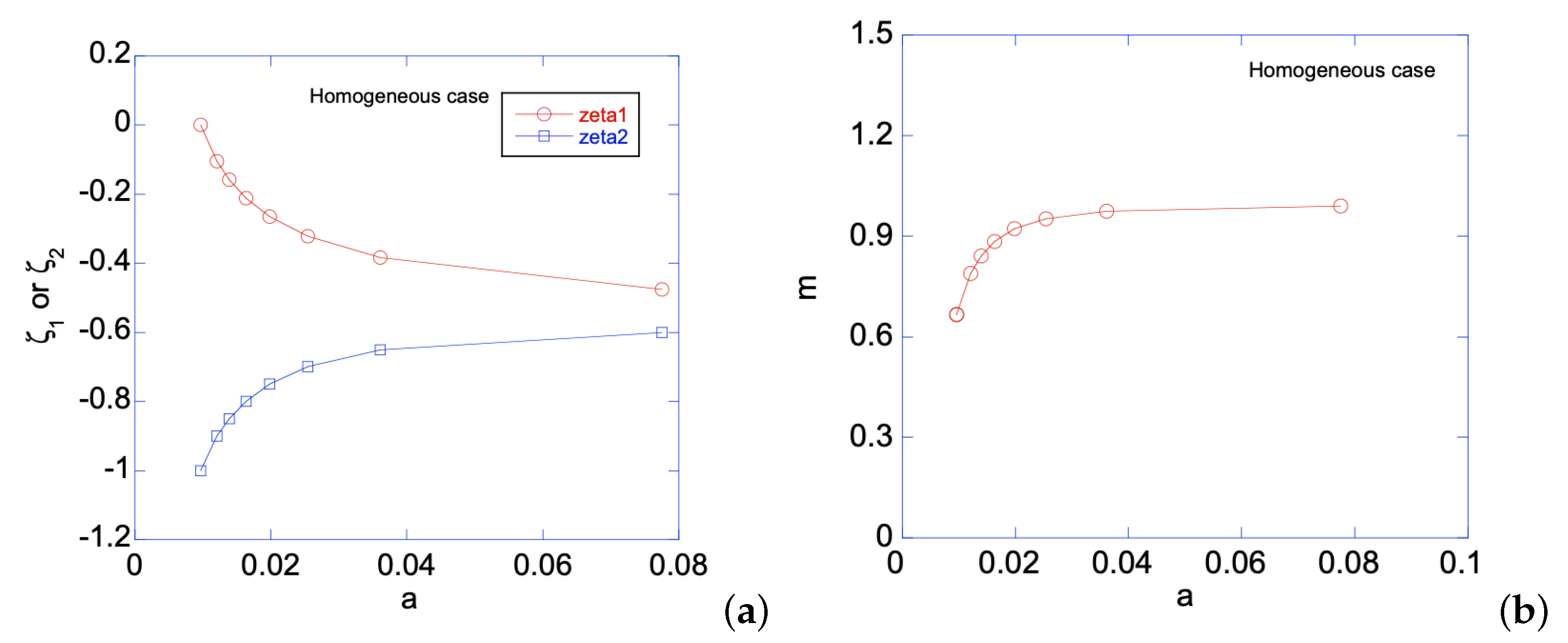
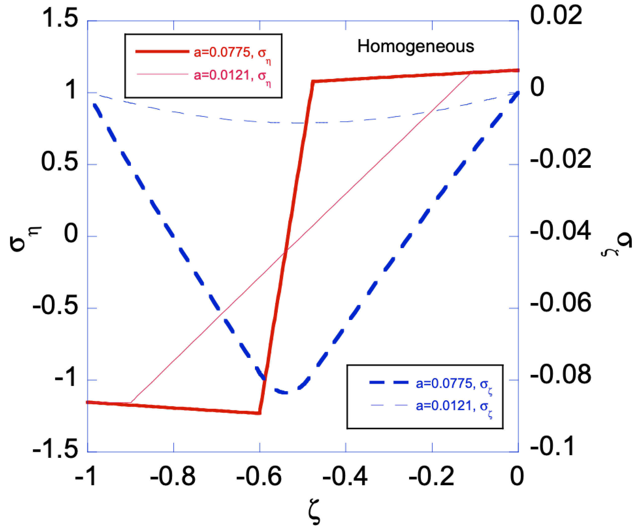
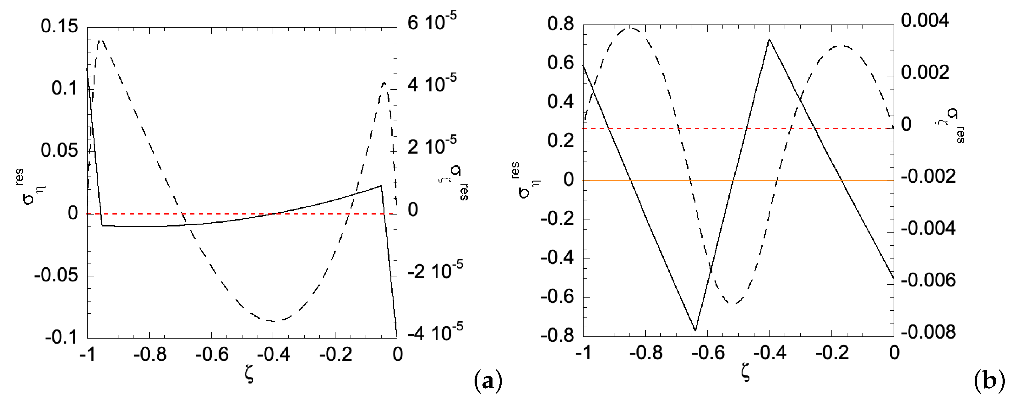
When the homogenous sheet is under bending, both edges will simultaneously develop plastic zones. Figure 3a shows the movement of the two elastic-plastic boundaries toward the centerline of the sheet, as deformation magnitude increases. The deformation magnitude is measured by parameter a. The applied bending moment is a function of a, as shown in Figure 3b. As an illustration of the developed analytical solutions in previous sections, Figure 4 shows the stress distributions along the sheet under two different deformation magnitudes. As can be seen, the plastic zones increase with a for , while remains in elastic regime. The reason for is not perfectly horizontal in the plastic zone is because our numerical codes do not allow N set equal to zero, hence a very small N is chosen, as shown in Table 1. After unloading, Figure 5a,b shows the residual stress distributions under two different as. Larger a increases the magnitude of residual stresses after unloading. Moreover, the residual stress is zero at the left and right edges, as indicated by the red short-dashed line.
5.2. FGM Sheet Belonged to Case (i) under Bending
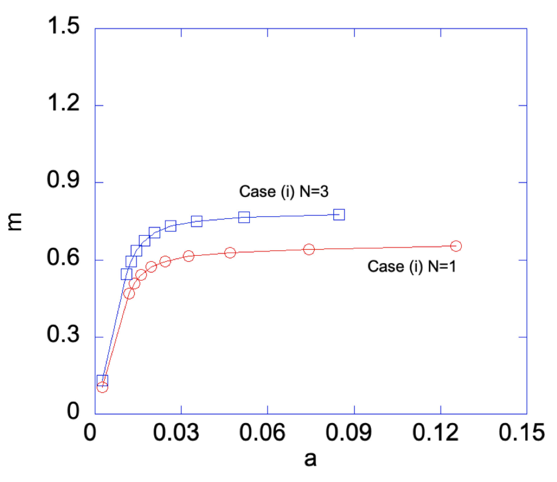
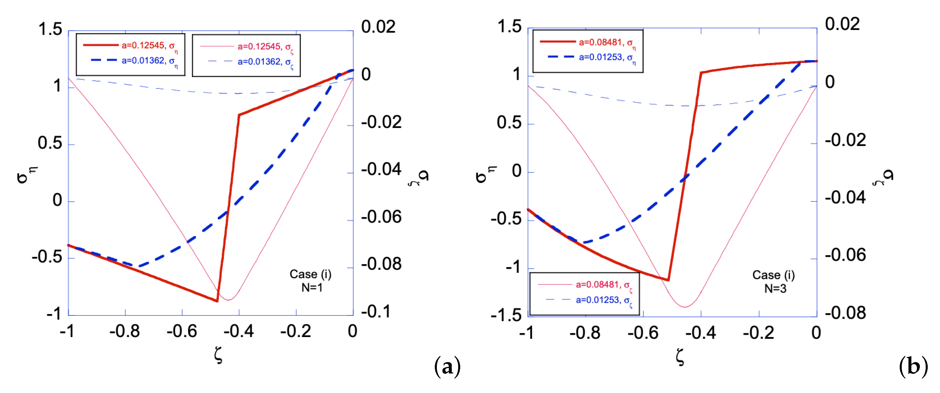
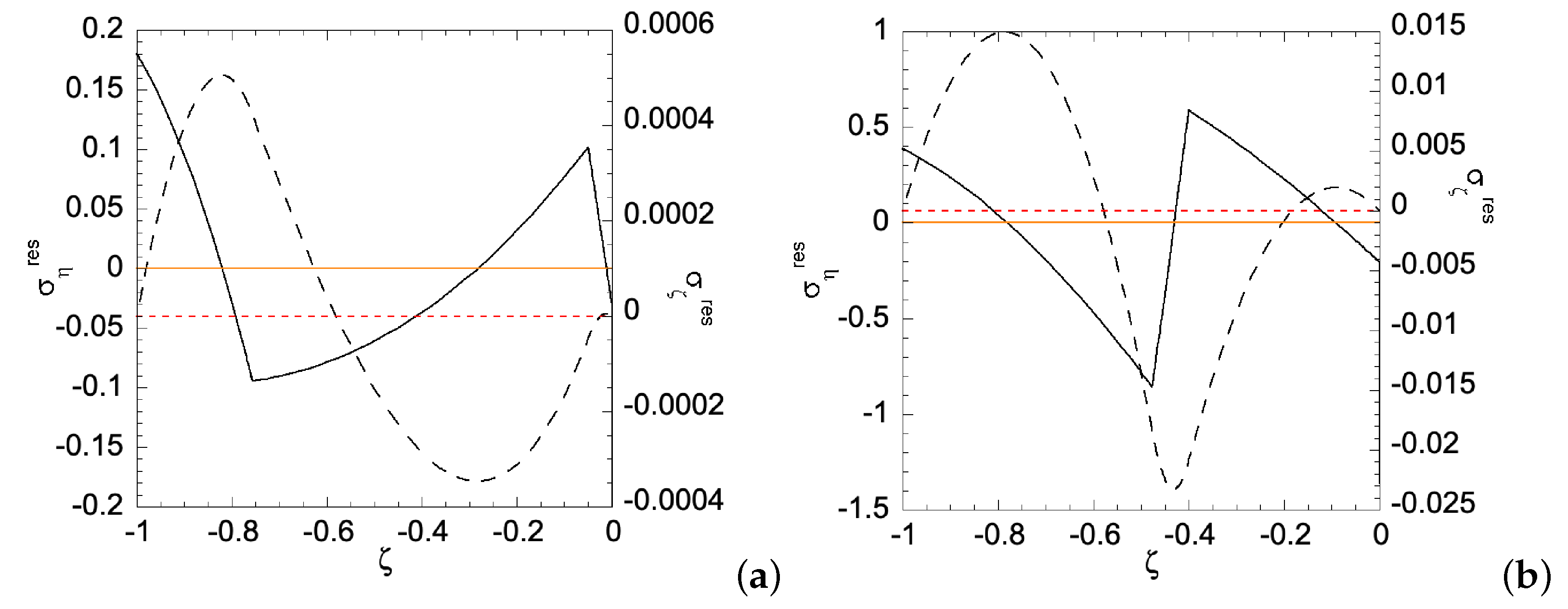
In Case (i), the left edge () of the sheet has smaller yield stress, hence a plastic zone will start on the left edge first. Figure 6 shows the relationship between the applied bending moment and deformation magnitude a with the gradient function exponent N = 1 and 3. As can be seen, larger m is required for than that for , as a increases. Under given deformation magnitudes, Figure 7 shows the stress distributions in the Case (i) FGM under plastic deformation. Larger plastic zone is developed at the left edge as deformation increases. After unloading, residual stress distributions are shown in Figure 8 and Figure 9 for the and FGM, respectively. Residual stresses are more predominant at the left edge. In addition, the residual stress is zero at the left and right edges, as indicated by the red short-dashed line.
5.3. FGM Sheet Belonged to Case (ii) under Bending
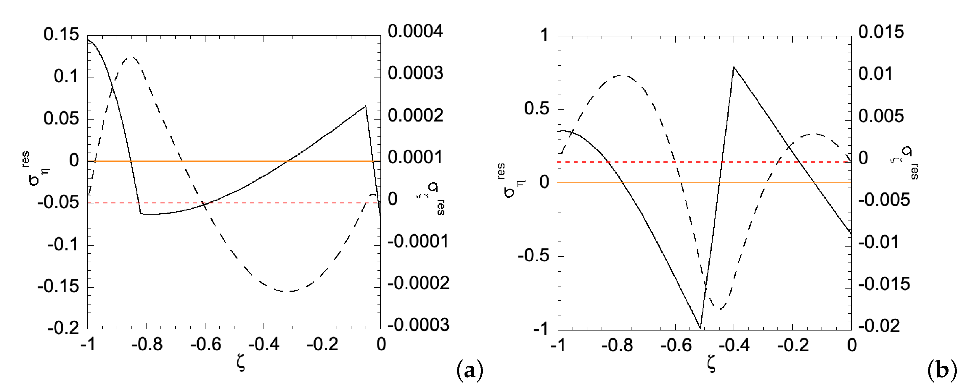
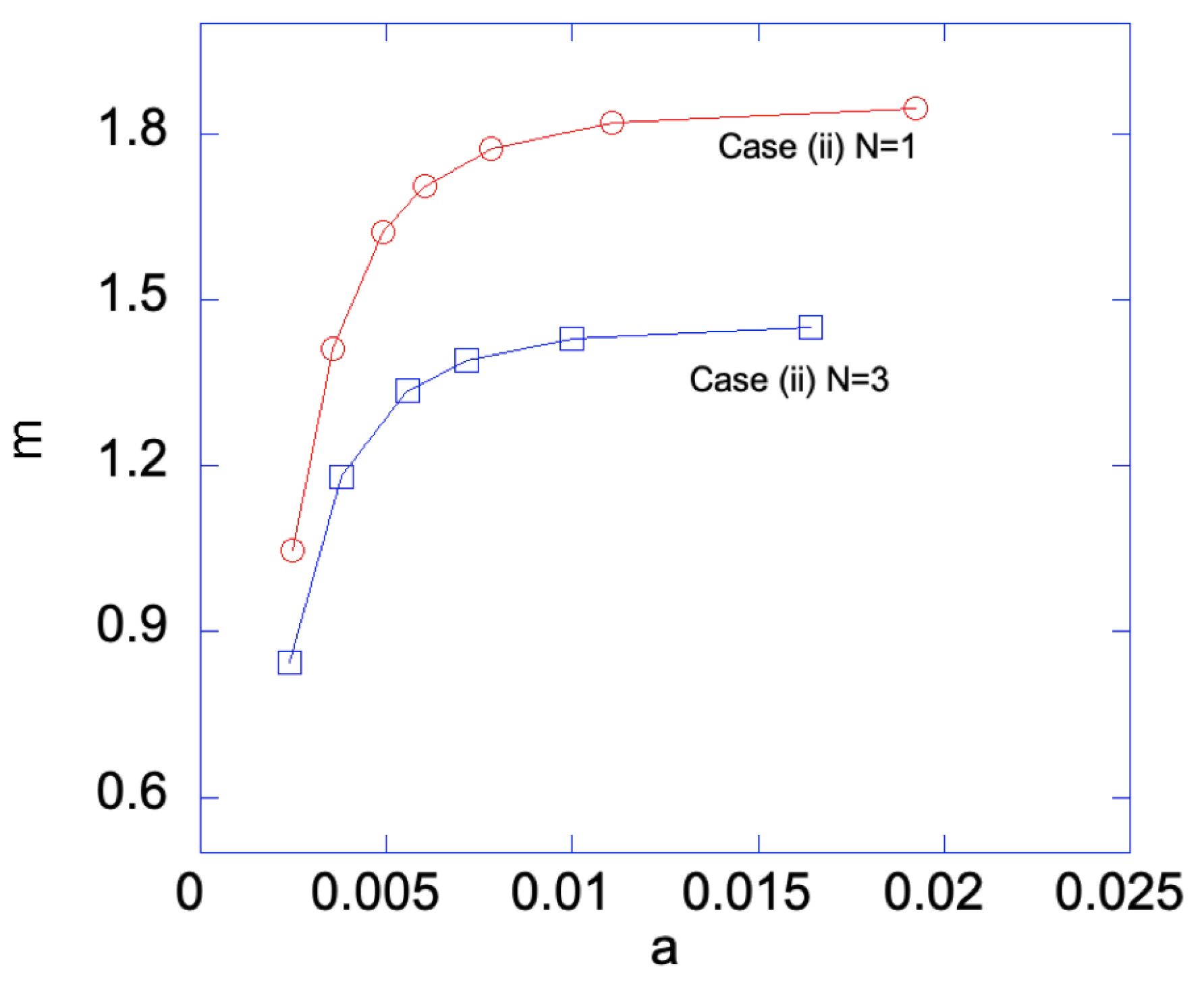
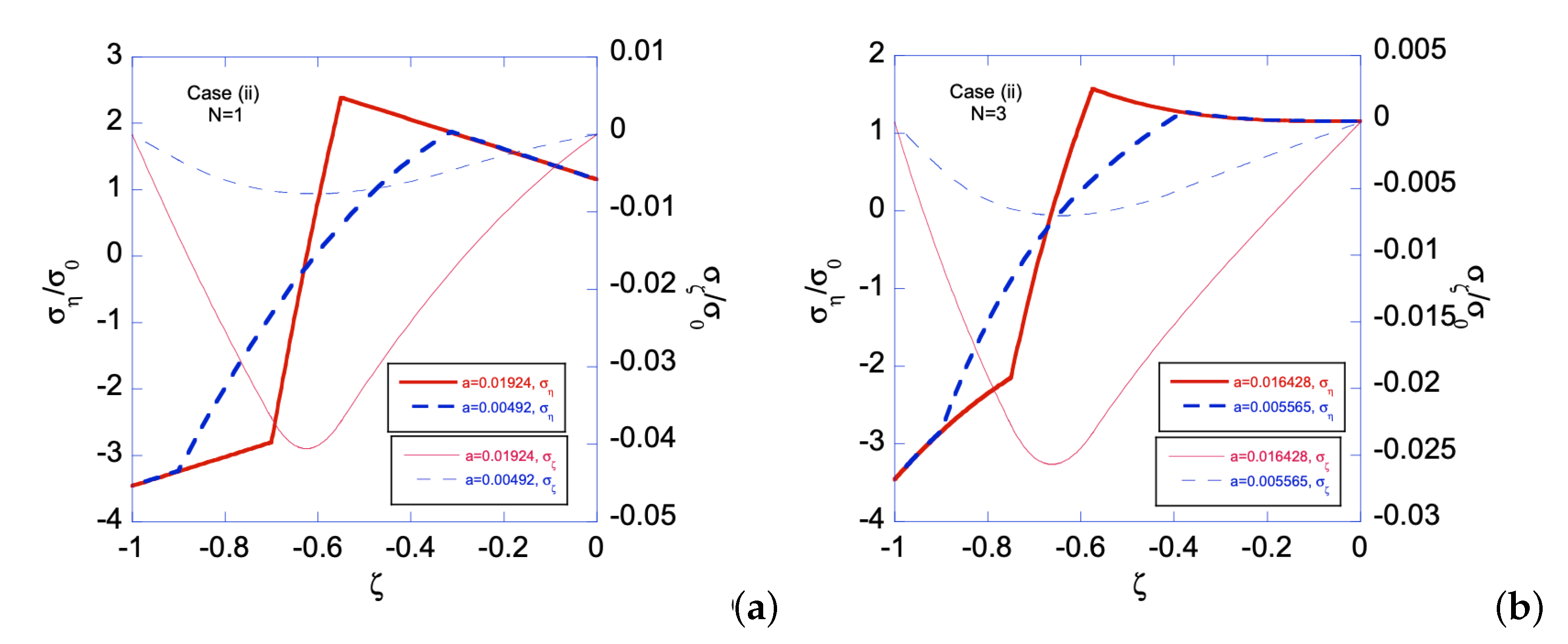
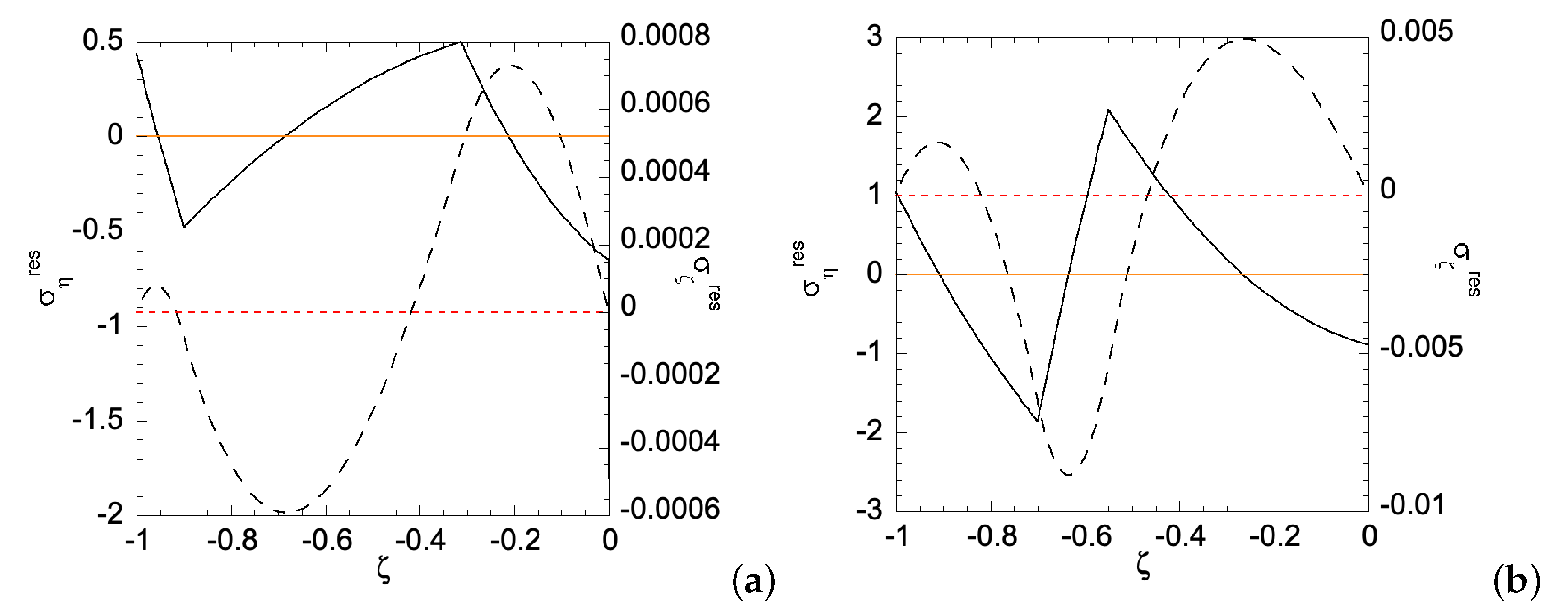
In Case (ii), the right edge () of the sheet has smaller yield stress, hence a plastic zone will start on the right edge first. Figure 10 shows the relationship between the applied bending moment and deformation magnitude a with the gradient function exponent N = 1 and 3. As can be seen, larger m is required for than that for , as a increases. Under given deformation magnitudes, Figure 11 shows the stress distributions in the Case (ii) FGM under plastic deformation. Larger plastic zone is developed at the right edge as deformation increases. After unloading, residual stress distributions are shown in Figure 12 and Figure 13 for the and FGM, respectively. Residual stresses are more predominant at the right edge. The residual stress is zero at the left and right edges, as indicated by the red short-dashed line. The results from the illustrative examples solved here may serve as benchmark solutions for data obtained from numerical or experimental methods.
6. Conclusions
Efficient analytical and numerical methods and procedures have been developed and programmed to predict the distribution of stresses in a sheet of incompressible material subject to plane strain pure bending at large strain and then the distribution of residual stresses after unloading. Springback is also predicted. It has been assumed that the sheet is made of functionally graded material. The general theory has been developed for an arbitrary through thickness distribution of material properties assuming that the initiation of plastic yielding occurs at one of the surfaces of the sheet. This assumption can be verified using the purely elastic solution (Equation (15)) and the yield criterion (Equation (7)). It is possible to use the general solutions (Equations (15), (18) and (25)) even if the assumption is not satisfied but constants of integration should be added. Then, these general solutions should be combined to satisfy the boundary conditions and the conditions at elastic/plastic boundaries. An illustrative example is concentrated on power law distributions of material properties. Using the numerical code developed in this work enables the effect of parameters involved in these laws to be predicted effectively. The calculated examples show the analytical solutions derived here can systematically treat the plastic problems of the homogenous or functionally graded sheet. The magnitudes of applied moment may be strongly influenced by the power law exponent as deformation increases, which provides an effective way to design the functionally graded sheets.
The method employed to derive the solution in this paper can be extended to cyclic loading. This new solution may be useful for the interpretation of experimental data from the reverse bending fatigue test (for example, [28]).
Author Contributions
Conceptualization, S.A., Y.-C.W. and L.L.; methodology, S.A. and Y.-C.W.; software, S.A. and Y.-C.W.; validation, S.A., Y.-C.W. and L.L.; formal analysis, S.A. and Y.-C.W.; investigation, S.A., Y.-C.W. and L.L.; resources, S.A., Y.-C.W. and L.L.; data curation, S.A. and Y.-C.W.; writing–original draft preparation, S.A., Y.-C.W. and L.L.; writing–review and editing, S.A., Y.-C.W. and L.L.; visualization, S.A. and Y.-C.W.; supervision, S.A., Y.-C.W. and L.L.; project administration, S.A., Y.-C.W. and L.L.; funding acquisition, S.A. and Y.-C.W.
Funding
S.A. acknowledges support from the Russian Foundation for Basic Research (Project 17-58-560005). This research was funded, in part, by Ministry of Science and Technology, Taiwan, grant number MOST 107-2221-E-006-028. This research was, in part, supported by the Ministry of Education, Taiwan, and the Aim for the Top University Project to the National Cheng Kung University (NCKU).
Acknowledgments
This work was initiated while Y.-C.W. was a visiting researcher at Beihang University, Beijing, China. Y.-C.W. is grateful to the National Center for High-performance Computing, Taiwan, for computer time and facilities.
Conflicts of Interest
The authors declare no conflict of interest.
References
- Birman, V.; Byrd, L.W. Modeling and analysis of functionally graded materials and structures. Appl. Mech. Rev. 2007, 60, 195–216. [Google Scholar] [CrossRef]
- Tutuncu, N.; Ozturk, M. Exact solutions for stresses in functionally graded pressure vessels. Compos. Part B Eng. 2001, 32, 683–686. [Google Scholar] [CrossRef]
- Akis, T. Elastoplastic analysis of functionally graded spherical pressure vessels. Comp. Mater. Sci. 2009, 46, 545–554. [Google Scholar] [CrossRef]
- Sadeghian, M.; Toussi, H.E. Axisymmetric yielding of functionally graded spherical vessel under thermos-mechanical loading. Comp. Mater. Sci. 2011, 50, 975–981. [Google Scholar] [CrossRef]
- Li, X.-Y.; Li, P.-D.; Kang, G.-Z. Axisymmetric thermo-elasticity field in a functionally graded circular plate of transversely isotropic material. Math. Mech. Solids 2013, 18, 464–475. [Google Scholar] [CrossRef]
- Horgan, C.O.; Chan, A.M. The pressurized hollow cylinder or disk problem for functionally graded isotropic linearly elastic materials. J. Elast. 1999, 55, 43–59. [Google Scholar] [CrossRef]
- Tutuncu, N. Stresses in thick-walled FGM cylinders with exponentially-varying properties. Eng. Struct. 2007, 29, 2032–2035. [Google Scholar] [CrossRef]
- You, L.H.; Wang, J.X.; Tang, B.P. Deformations and stresses in annular disks made of functionally graded materials subjected to internal and/or external pressure. Meccanica 2009, 44, 283–292. [Google Scholar] [CrossRef]
- Jabbari, M.; Sohrabpour, S.; Eslami, M.R. Mechanical and thermal stresses in a functionally graded hollow cylinder due to radially symmetric loads. Int. J. Press. Vessels Pip. 2002, 79, 493–497. [Google Scholar] [CrossRef]
- Eraslan, A.N.; Akis, T. Plane strain analytical solutions for a functionally graded elastic–plastic pressurized tube. Int. J. Press. Vessels Pip. 2006, 83, 635–644. [Google Scholar] [CrossRef]
- Horgan, C.O.; Chan, A.M. The stress response of functionally graded isotropic linearly elastic rotating disks. J. Elast. 1999, 55, 219–230. [Google Scholar] [CrossRef]
- Peng, X.-L.; Li, X.-F. Effects of gradient on stress distribution in rotating functionally graded solid disks. J. Mech. Sci. Technol. 2012, 26, 1483–1492. [Google Scholar] [CrossRef]
- Bayat, M.; Saleem, M.; Sahari, B.B.; Hamouda, A.M.S.; Mahdi, E. Analysis of functionally graded rotating disks with variable thickness. Mech. Res. Commun. 2008, 35, 283–309. [Google Scholar] [CrossRef] [Green Version]
- Peng, X.-L.; Li, X.-F. Elastic analysis of rotating functionally graded polar orthotropic disks. Int. J. Mech. Sci. 2012, 60, 84–91. [Google Scholar] [CrossRef]
- Dai, H.-L.; Dai, T.; Zheng, H.-Y. Stresses distributions in a rotating functionally graded piezoelectric hollow cylinder. Meccanica 2012, 47, 423–436. [Google Scholar] [CrossRef]
- Callioglu, H.; Sayer, M.; Demir, E. Elastic–plastic stress analysis of rotating functionally graded discs. Thin-Walled Struct. 2015, 94, 38–44. [Google Scholar] [CrossRef]
- Elishakoff, I.; Pentaras, D.; Gentilini, C. Mechanics of Functionally Graded Material Structures; World Scientific: Singapore, 2016; ISBN 978-981-4656-58-0. [Google Scholar]
- Alexandrov, S.; Kim, J.-H.; Chung, K.; Kang, T.-J. An alternative approach to analysis of plane-strain pure bending at large strains. J. Strain Anal. Eng. Des. 2006, 41, 397–410. [Google Scholar] [CrossRef]
- Hill, R. The Mathematical Theory of Plasticity; Clarendon Press: Oxford, UK, 1950; ISBN 0-19-850367-9. [Google Scholar]
- Alexandrov, S.; Hwang, Y.-M. The bending moment and springback in pure bending of anisotropic sheets. Int. J. Solids Struct. 2009, 46, 4361–4368. [Google Scholar] [CrossRef] [Green Version]
- Alexandrov, S.; Hwang, Y.-M. Plane strain bending with isotropic strain hardening at large strains. Trans. ASME J. Appl. Mech. 2010, 77, 064502. [Google Scholar] [CrossRef]
- Alexandrov, S.; Gelin, J.-C. Plane strain pure bending of sheets with damage evolution at large strains. Int. J. Solids Struct. 2011, 48, 1637–1643. [Google Scholar] [CrossRef] [Green Version]
- Alexandrov, S.; Hwang, Y.-M. Influence of Bauschinger effect on springback and residual stresses in plane strain pure bending. Acta Mech. 2011, 220, 47–59. [Google Scholar] [CrossRef]
- Verguts, H.; Sowerby, R. The pure plastic bending of laminated sheet metals. Int. J. Mech. Sci. 1975, 17, 31–51. [Google Scholar] [CrossRef]
- Romano, G.; Barretta, R.; Diaco, M. Geometric continuum mechanics. Meccanica 2014, 49, 111–133. [Google Scholar] [CrossRef]
- Nakumura, T.; Wang, T.; Sampath, S. Determination of properties of graded materials by inverse analysis and instrumented indentation. Acta Mater. 2000, 48, 4293–4306. [Google Scholar] [CrossRef]
- Huang, H.; Chen, B.; Han, Q. Investigation on buckling behaviors of elastoplastic functionally graded cylindrical shells subjected to torsional loads. Comput. Struct. 2014, 118, 234–240. [Google Scholar] [CrossRef]
- Faghidian, S.A.; Jozie, A.; Sheykhloo, M.J.; Shamsi, A. A novel method for analysis of fatigue life measurements based on modified Shepard method. Int. J. Fatigue 2014, 68, 144–149. [Google Scholar] [CrossRef]
Figure 1.
Geometric configuration of the bending problem: (a) before deformation; and (b) after deformation.
Figure 1.
Geometric configuration of the bending problem: (a) before deformation; and (b) after deformation.

Figure 2.
Schematics of elastic and plastic zones.

Figure 3.
For the homogeneous sheet under bending: (a) or vs. a; and (b) applied bending moment m vs. a.
Figure 3.
For the homogeneous sheet under bending: (a) or vs. a; and (b) applied bending moment m vs. a.

Figure 4.
Stress distributions for the bent homogenous sheet with two different loading conditions and . Two plastic zones, one developed from the left edge and the other from the right edge, increase their size as a increases for .
Figure 4.
Stress distributions for the bent homogenous sheet with two different loading conditions and . Two plastic zones, one developed from the left edge and the other from the right edge, increase their size as a increases for .

Figure 5.
Residual stress distribution along the homogeneous sheet for: (a) ; and (b) . Solid line is for residual and dashed line for residual . Zeros of and are indicated by orange solid line and red dashed line, respectively.
Figure 5.
Residual stress distribution along the homogeneous sheet for: (a) ; and (b) . Solid line is for residual and dashed line for residual . Zeros of and are indicated by orange solid line and red dashed line, respectively.

Figure 6.
Bending moment m vs. a for Case (i) with and . With sufficiently large deformation, i.e., large a, Case (iii) is automatically developed, hence both edges are plastically deformed.
Figure 6.
Bending moment m vs. a for Case (i) with and . With sufficiently large deformation, i.e., large a, Case (iii) is automatically developed, hence both edges are plastically deformed.

Figure 7.
Stress distributions for Case (i) with N = 1 with two different deformation magnitudes, i.e., two different as, for: (a) ; and (b) . Two plastic zones, one developed from the left edge and the other from the right edge, increase their size as a increases for .
Figure 7.
Stress distributions for Case (i) with N = 1 with two different deformation magnitudes, i.e., two different as, for: (a) ; and (b) . Two plastic zones, one developed from the left edge and the other from the right edge, increase their size as a increases for .

Figure 8.
Residual stress distributions for Case (i) with N = 1 under deformation: (a) ; and (b) . Solid line is for residual and dashed line for residual . Zeros of and are indicated by orange solid line and red dashed line, respectively.
Figure 8.
Residual stress distributions for Case (i) with N = 1 under deformation: (a) ; and (b) . Solid line is for residual and dashed line for residual . Zeros of and are indicated by orange solid line and red dashed line, respectively.

Figure 9.
Residual stress distributions for Case (i) with N = 3 under deformation: (a) ; and (b) . Solid line is for residual and dashed line for residual . Zeros of and are indicated by orange solid line and red dashed line, respectively.
Figure 9.
Residual stress distributions for Case (i) with N = 3 under deformation: (a) ; and (b) . Solid line is for residual and dashed line for residual . Zeros of and are indicated by orange solid line and red dashed line, respectively.

Figure 10.
Bending moment m vs. a for Case (ii) with and . With sufficiently large deformation, i.e., large a, Case (iii) is developed, hence both edges are plastically deformed.
Figure 10.
Bending moment m vs. a for Case (ii) with and . With sufficiently large deformation, i.e., large a, Case (iii) is developed, hence both edges are plastically deformed.

Figure 11.
Stress distributions for Case (ii) with two different deformation magnitudes, i.e., two different as, for: (a) ; and (b) . Two plastic zones, one developed from the left edge and the other from the right edge, increase their size as a increases for .
Figure 11.
Stress distributions for Case (ii) with two different deformation magnitudes, i.e., two different as, for: (a) ; and (b) . Two plastic zones, one developed from the left edge and the other from the right edge, increase their size as a increases for .

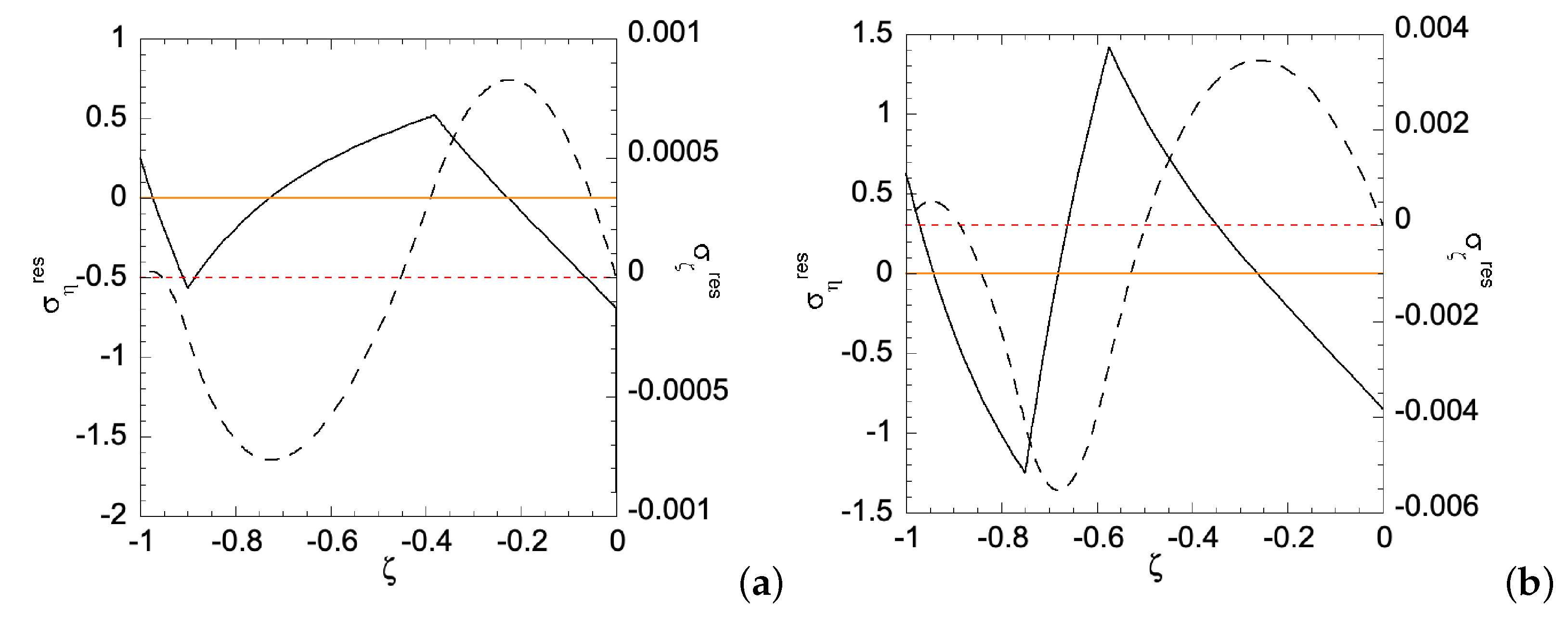
Figure 12.
Residual stress distributions for Case (ii) with under deformation: (a) ; and (b) . Solid curve is for residual and dashed curve for residual . Zeros of and are indicated by orange solid line and red dashed line, respectively.
Figure 12.
Residual stress distributions for Case (ii) with under deformation: (a) ; and (b) . Solid curve is for residual and dashed curve for residual . Zeros of and are indicated by orange solid line and red dashed line, respectively.

Figure 13.
Residual stress distributions for Case (ii) with under deformation: (a) ; and (b) . Solid curve is for residual and dashed curve for residual . Zeros of and are indicated by orange solid line and red dashed line, respectively.
Figure 13.
Residual stress distributions for Case (ii) with under deformation: (a) ; and (b) . Solid curve is for residual and dashed curve for residual . Zeros of and are indicated by orange solid line and red dashed line, respectively.


Table 1.
Material parameters used in the numerical examples.
| , GPa | , GPa | , GPa | , GPa | N | |
|---|---|---|---|---|---|
| Homogeneous | 30 | 30 | 1 | 1 | 0.0001 |
| FGM Case (i) | 30 | 10 | 1 | 0.1 | 1 |
| FGM Case (i) | 30 | 10 | 1 | 0.1 | 3 |
| FGM Case (ii) | 10 | 30 | 0.1 | 1 | 1 |
| FGM Case (ii) | 10 | 30 | 0.1 | 1 | 3 |
© 2019 by the authors. Licensee MDPI, Basel, Switzerland. This article is an open access article distributed under the terms and conditions of the Creative Commons Attribution (CC BY) license (http://creativecommons.org/licenses/by/4.0/).
Share and Cite
MDPI and ACS Style
Alexandrov, S.; Wang, Y.-C.; Lang, L. A Theory of Elastic/Plastic Plane Strain Pure Bending of FGM Sheets at Large Strain. Materials 2019, 12, 456. https://doi.org/10.3390/ma12030456
AMA Style
Alexandrov S, Wang Y-C, Lang L. A Theory of Elastic/Plastic Plane Strain Pure Bending of FGM Sheets at Large Strain. Materials. 2019; 12(3):456. https://doi.org/10.3390/ma12030456
Chicago/Turabian StyleAlexandrov, Sergey, Yun-Che Wang, and Lihui Lang. 2019. "A Theory of Elastic/Plastic Plane Strain Pure Bending of FGM Sheets at Large Strain" Materials 12, no. 3: 456. https://doi.org/10.3390/ma12030456
Note that from the first issue of 2016, this journal uses article numbers instead of page numbers. See further details here.