New Shape Function for the Bending Analysis of Functionally Graded Plate
by
 ,
,
Dragan Čukanović
1, 
Aleksandar Radaković
2,*,
Gordana Bogdanović
3,
Milivoje Milanović
2,
Halit Redžović
2 and
Danilo Dragović
2 1
Faculty of Technical Sciences, University of Priština, 38220 Kosovska Mitrovica, Serbia
2
Department of Technical Sciences, State University of Novi Pazar, 36300 Novi Pazar, Serbia
3
Faculty of Engineering, University of Kragujevac, 34000 Kragujevac, Serbia
*
Author to whom correspondence should be addressed.
Materials 2018, 11(12), 2381; https://doi.org/10.3390/ma11122381
Submission received: 2 November 2018
/
Revised: 18 November 2018
/
Accepted: 22 November 2018
/
Published: 26 November 2018
(This article belongs to the Special Issue Advances in Mechanical Problems of Functionally Graded Materials and Structures)
Abstract
:The bending analysis of thick and moderately thick functionally graded square and rectangular plates as well as plates on Winkler–Pasternak elastic foundation subjected to sinusoidal transverse load is presented in this paper. The plates are assumed to have isotropic, two-constituent material distribution through the thickness, and the modulus of elasticity of the plate is assumed to vary according to a power-law distribution in terms of the volume fractions of the constituents. This paper presents the methodology of the application of the high order shear deformation theory based on the shape functions. A new shape function has been developed and the obtained results are compared to the results obtained with 13 different shape functions presented in the literature. Also, the validity and accuracy of the developed theory was verified by comparing those results with the results obtained using the third order shear deformation theory and 3D theories. In order to determine the procedure for the analysis and the prediction of behavior of functionally graded plates, the new program code in the software package MATLAB has been developed based on the theories studied in this paper. The effects of transversal shear deformation, side-to-thickness ratio, and volume fraction distributions are studied and appropriate conclusions are given.
1. Introduction
Failure and delamination at the border between two layers are the biggest and the most frequently studied problem of the conventional composite laminates. Delamination of layers due to high local inter-laminar stresses causes a reduction of stiffness and a loss of structural integrity of a construction. In order to eliminate these problems, improved materials such as functionally graded materials (FGM), which are getting more and more popular, are used for innovative engineering constructions.
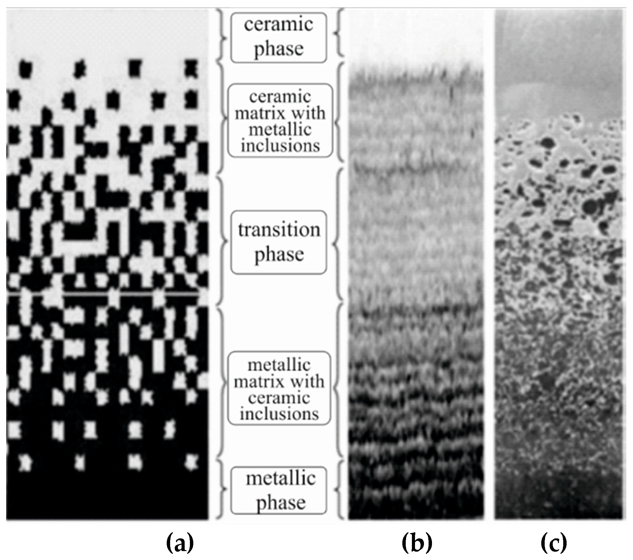
FGM is a composite material consisting of two or more constituents with the continuous change of properties in a certain direction. In other words, these materials can also be defined as materials which possess a gradient change of properties due to material heterogeneity. A gradient property can go in one or more directions and it can also be continuous or discontinuous from one surface to another depending on the production technique [1,2,3]. One of the most common uses of FGM materials is found in thermal barriers, one surface of which is in contact with high temperatures and is made of ceramic which can provide adequate thermal stability, low thermal conductivity, and fine antioxidant properties. The low-temperature side of the barrier is made of metal, which is superior in terms of mechanical strength, toughness, and high thermal conductivity. Functionally graded materials, which contain metal and ceramic constituents, improve thermo-mechanical properties between layers, because of which delamination of layers should be avoided due to continuous change between properties of the constituents. By varying the percentage of volume fraction content of the two or more materials, FGM can be formed so that it achieves a desired gradient property in specific directions. Figure 1 shows schematic of continuously graded microstructure with metal-ceramic constituents [4].
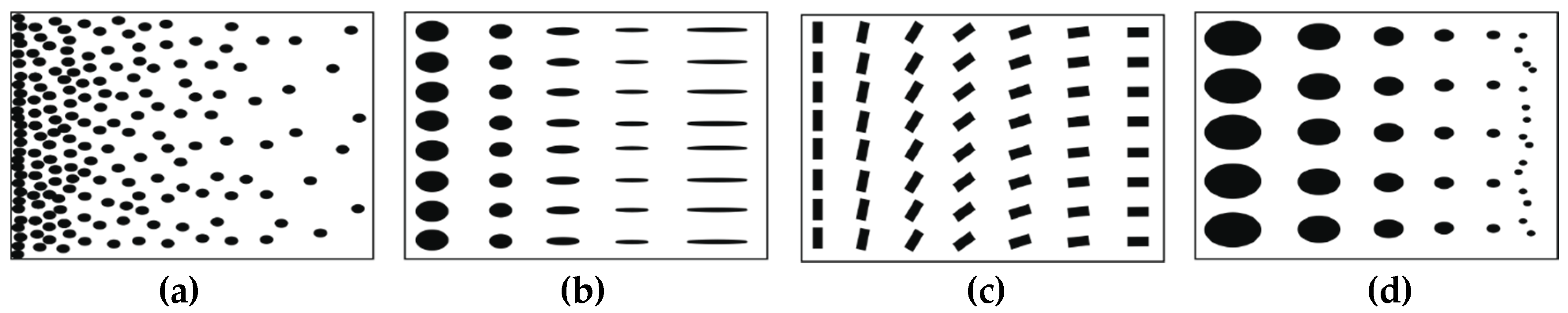
Depending on the nature of gradient, functionally graded materials may be grouped into fraction gradient type, shape gradient type, orientation gradient type and size gradient type (Figure 2) [5].
With the expansion of the FGM material application area, it was necessary to improve fabrication methods for mentioned materials. Various fabrication methods have been developed for the preparation of bulk FGMs and graded thin films. The processing methods are commonly classified into four groups like powder technology methods (dry powder processing, slip vesting, tape casting, infiltration process or electrochemical gradation, powder injection molding and self-propagating high temperature synthesis, etc.), deposition methods (chemical vapor deposition, physical vapor deposition, electrophoretic deposition, slurry deposition, pulsed laser deposition, plasma spraying, etc.), in-situ processing methods (laser cladding, spray forming, sedimentation and solidification, centrifugal casting, etc.), and rapid prototyping processes (multiphase jet solidification, 3D-printing, laser printing, laser sintering, etc.) [6]. The basic difference between the mentioned production methods can be made according to whether the obtained materials have a stepwise or continuous structure. The main disadvantage of the methods based on powder metallurgy is that it is very difficult to obtain FGM with a continuous change in properties. Continuous graded structures are produced by methods based on casting. Taking this fact into consideration, it was necessary to develop functions which would, with a smaller degree of approximation and in the best way possible, describe a gradient change of properties in a desired direction [7,8].
The majority of already existing software for the analysis of the composite materials are based on the classical plate theory (CPT) [9] and first-order shear deformation theories (FSDT), which were developed by Mindlin [10] and, in a similar way, by Reissner [11,12]. Although classical theory does not consider the effect of transverse shear stresses, it can provide acceptable predictions of the behavior and the results for thin FGM plates where the effects of shear and normal strains across the thickness of the plate are negligible.
Static problems of buckling and bending of FGM plates by using the CPT for different cases of boundary conditions were studied by the authors of the following papers [13,14,15]. Considering von Karman’s type of geometric nonlinearity, FGM behavior was analyzed in [16,17]. The effect of a gradient distribution of materials in thin square and rectangular FGM plates was studied in terms of different cases of dynamic load. The papers [18,19] analyze free vibrations of the FGM plates using CPT for different boundary conditions in the area of geometric linearity. Von Karman’s type of nonlinearity has been used in the papers [20,21].
Mindlin’s and Reissner’s theories take into consideration the effect of shear stresses across the thickness of the plate and require the use of correctional factors which generally depend on the shape and geometry. FSDT theory has been widely used in numerous papers mainly for solving nonlinear problems [22,23]. Static problems due to introducing geometric nonlinearity have been studied in [24], using Green’s strain tensor, and in [25] using von Karman’s strain tensor.
In order to avoid the use of shear correctional factors, high-order shear deformation theories (HSDT) have been introduced. HSDT theories can be developed by developing displacement components into power series at the coordinate of thickness. Generally, in the theories developed in this way, desired precision of the analysis can be achieved by introducing a sufficient number of terms in the power series. The most frequently used HSDT theory is the third-order shear deformation theory (TSDT) developed for composite laminates [26,27], which takes into consideration the effects of shear strains by satisfying the condition of keeping the upper and lower surface of the laminates free of stresses. Later, that theory was used in the analysis of FGM plates [28,29] for solving buckling problems [30,31], free vibrations and dynamic stability [32,33]. In addition to TSDT, there are HSDT theories based on the shape functions which represent a special group of HSDT theories introduced in order to eliminate the need for correctional factors [34,35]. Contrary to CPT and FSDT, the supposed displacement shapes in this theory do not foresee that the normal to the middle plane of the laminate plate remain a straight line, but that during deformation the normal will become curved. Generally, shape functions can be polynomial, hyperbolic, exponential, parabolic etc. Polynomial HSDTs usually diverge from other types of these theories and in accordance to the order of a polynomial at the thickness coordinate they are categorized into the group of second-order shear deformation theories (SSDT) or third-order shear deformation theories. Polynomial theories are those that are most common in the articles, which deal with FG plates’ analysis using HSDT. According to [36,37] all polynomial HSDT of third order can be classified so that the supposed displacement fields contain eleven unknowns. The above-mentioned formulation has been expanded in [38,39] by supposing that the displacements are cubic functions of the thickness coordinate of the plate, that is, the supposed displacements contain twelve independent variables. In [40,41,42] the authors have proposed a shear deformation theory of n-series, which was obtained by modifying the displacement field of TSDT, in order to explain polynomial elements of n-series. Unlike HSDT based on polynomial shape functions, some authors have dealt with researching and introducing different hyperbolic, exponential, parabolic, and other shape functions [43,44,45,46,47,48,49,50,51]. Proposed functions were applied in the analysis of conventional laminate composites with the aim to describe the behavior of moderately thick and thick under different static and dynamic loads.
On the other hand, continuum-based 3D elasticity theory could be used for the analysis of these plates. However, 3D solution methods are mathematically complex which consequently results in prolonged calculation time and the need for high performance hardware. Taking the aforementioned into consideration, developing and using 2D shear deformation plate theories, which consider the effects of previously mentioned shear and normal strains and provide the precision in the same way as 3D models do, represents a trend in the process of analysis of FGM plates.
This paper presents, in detail, the methodology of the application of the HSDT theory based on the shape functions. A new shape function has been developed and the obtained results are compared to the results obtained with 13 different shape functions presented in the papers from the reference list. Also, the results have been verified through comparison with the results obtained with TSDT and 3D theories. In order to determine a procedure for the analysis and the prediction of behavior of FGM plates, the new program code in the software package MATLAB (MATrix LABoratory) has been developed based on theories studied in this paper.
Finally, the ultimate goal and the purpose of all the previously mentioned studies and analyses is the application of FGM in different areas of engineering and branches of industry. Although FGM were initially used as materials for thermal barrier in space shuttles, today they are becoming widely used in the field of medicine, dentistry, energy and nuclear sector, automotive industry, military, optoelectronics etc.
2. Description of the Problem
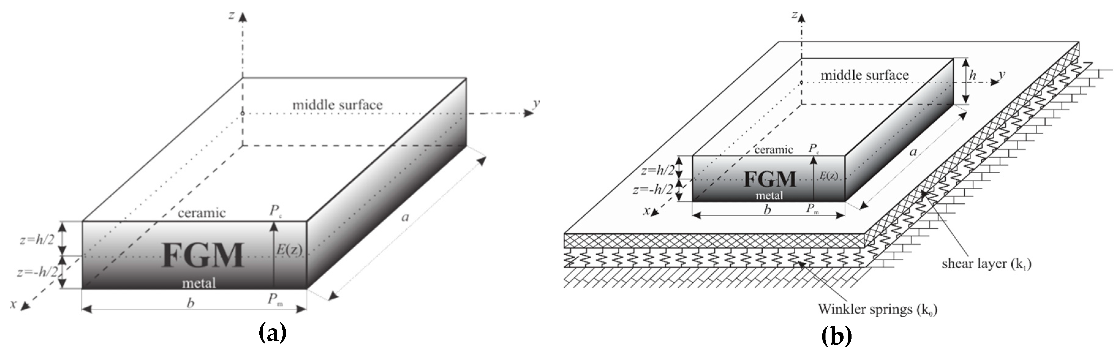
The subject of the analysis in this paper are FGM plate (Figure 3a) and FGM plate on elastic foundation (Figure 3b). The plate (length a, width b and height h) is made of functionally graded material consisting of the two constituents, namely, metal and ceramics.
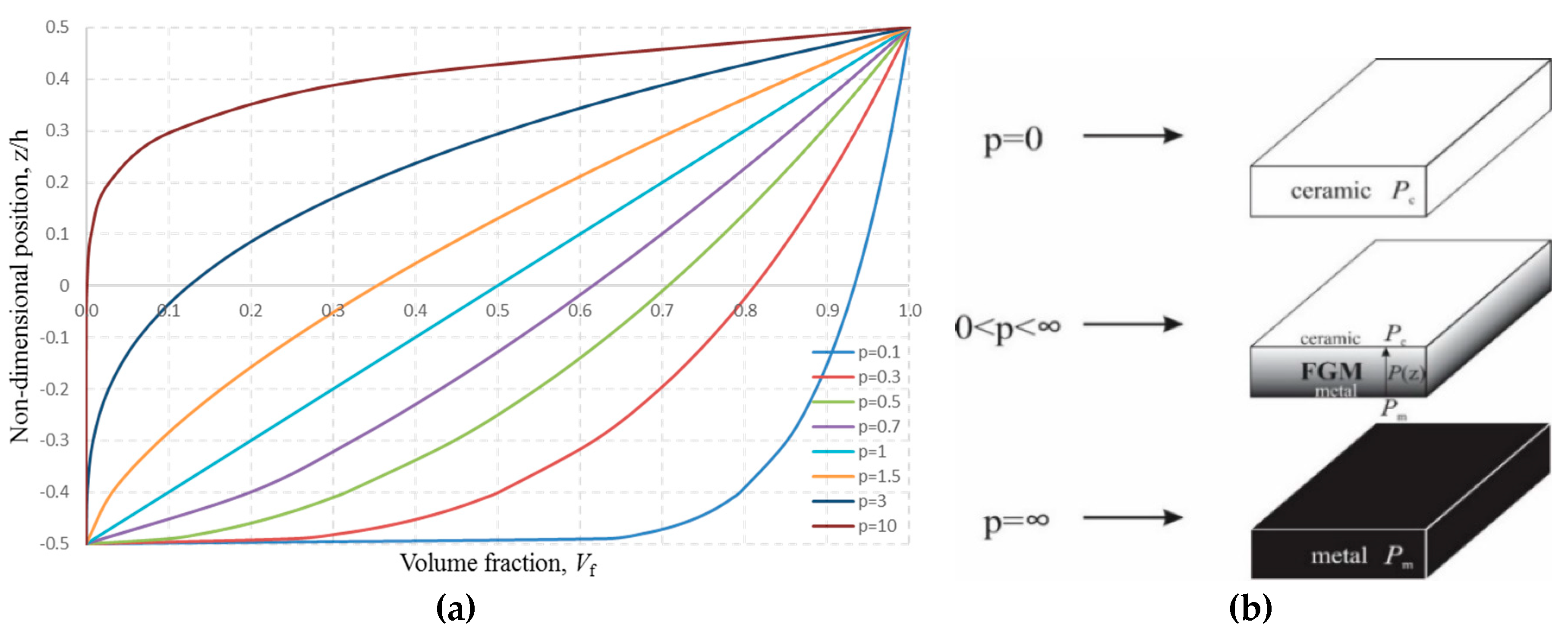
It is assumed that mechanical properties of the FGM in the thickness direction of the plate change according to the power law distribution (Figure 4a):
This law defines the change of the mechanical properties as the function of the volume fraction of the FGM constituents in the thickness direction of the plate.
In the Equation (1), h represents total thickness of the plate, and P(z) represents a material property in an arbitrary cross-section z, −h/2 < z < h/2. Pc represents the material property at the top of the plate z = h/2 − ceramic, and Pm represents the material property at the bottom of the plate z = −h/2 − metal. Index p is the exponent of the equation which defines the volume fraction of the constituents in FGM. Practically, by varying the index p, homogenous plates as well as FGM plate with precisely determined gradient structure could be obtained, as it is presented in Figure 4b:
- when p = 0 the plate is homogenous, made of ceramics,
- when 0 < p < ∞ the plate has a gradient structure,
- theoretically, when p = ∞ the plate becomes homogenous again, made of metal, although the plate can be considered homogenous even when p > 20.
3. Kinematic Displacement-Strain Relations and Constitutive Equation of Elasticity for FGM
According to HSDT based on the shape functions, displacements could be presented in the following way:
where: are displacement components in the middle plane of the plate, are rotation angles of transverse normal in relation to x and y axes, respectively, are rotations of the transverse normal due to transverse shear and is the shape function.
In the reference literature there are many shape functions which can be polynomial, trigonometric, exponential, hyperbolic. Some examples of the shape functions are given in Table 1.
This paper proposes a new shape function as follows:
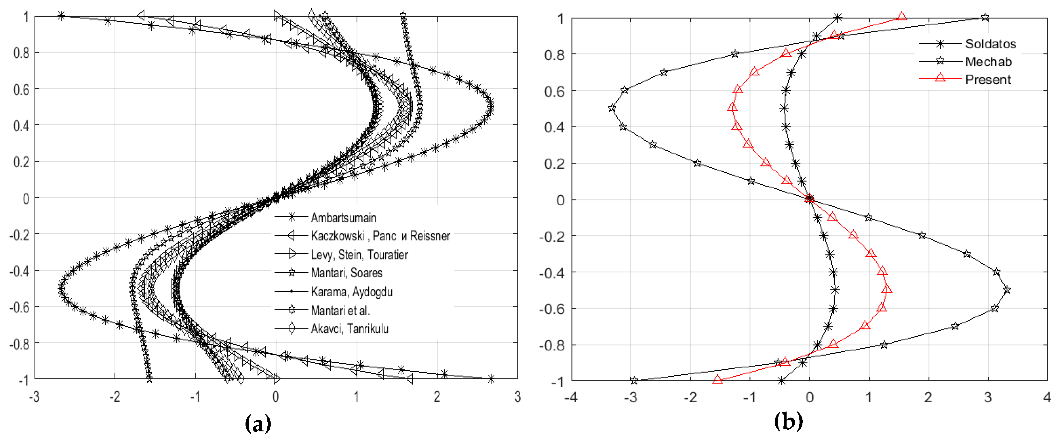
The introduced shape function is an odd function of the thickness coordinate z and satisfies zero stress conditions for out of plane shear stresses. Observing the shape functions in the Table 1, may see that the proposed function belongs to the group of simple mathematic functions. This fact makes the integration process easier and thus reduces considerably the calculation time. Having in mind that the function is analytically integrable, there is no need to switch to numeric integration, which additionally increases the precision of the obtained results. The verification of the above claims is shown in the comparative diagrams (Figure 5) of the newly introduced shape function and the shape functions given in the Table 1. These shape functions’ diagrams can be categorized into two groups of functions. In both cases it can be seen in the diagram that, in the case of the ratio z/h = 0.5, all shape functions have extreme values, which are different (Figure 5a). The proposed new shape function (3) belongs to the second group (Figure 5b), together with the functions of Soldatos and Mechab which are also analytically integrable functions.
For small displacements and moderate rotations of a transverse normal in relation to x axis and y axis, normal and shear strain components are obtained by well-known relations in linear elasticity between displacements and strains:
where:
where is the first derivative of the shape function in the thickness direction of the plate.
The elastic constitutive relations for FGM are given as follows:
where the coefficients of the constitutive elasticity tensor could be defined through engineering constants:
Due to the gradient change of the plate structure in the direction of the z coordinate, based on (1), the modulus of elasticity could be defined as:
while Poisson’s ratio is considered constant due to a small value variation in the thickness direction of the plate, .
As it could be seen, the coefficients of the constitutive tensor are functionally dependent on the z coordinate which practically means that for there is a finite number of planes parallel to the middle plane, where each of these planes has different values of the constitutive tensor .
4. Bending of FGM Plates and FGM Plates on Elastic Foundation
It is assumed that the plate is loaded with an arbitrary transverse load . Work under external load is defined as:
where:
is the sinusoidal transverse load with an amplitude .
Plate strain energy is defined as:
where force, moments and higher order moments vectors are obtained in the following form:
Matrices in the developed form could be presented in the following way:
In the Equation (12) by grouping the terms with the elements of constitutive tensor, new matrices with the following components could be defined:
Therefore, load vectors could now be defined in the following form:
By exchanging plate strain energy (11) and work under external load (9) into the equation which defines the minimum total potential energy principle:
The following form is obtained:
By exchanging the strain components (5) and by applying the calculus of variations, the following equilibrium equations are obtained:
which could be further solved through analytical and numerical methods.
In the case of a plate on elastic foundation, in the Equation (16) deformation energy of the elastic foundation should be taken into consideration, which is defined using Winkler–Pasternak model in the following way:
Using the previously mentioned the minimum total potential energy principle, the equilibrium equations of the plate on elastic foundation are the following:
5. Analytical Solution of the Equilibrium Equations
Although analytical solution methods are limited to simple geometrical problems, boundary conditions and loads, they can provide a clear understanding of the physical aspect of the problem and its solutions are very precise. Since analytical solutions are extremely important for developing new theoretical models, primarily due to their understanding of the physical aspects of the problem, and considering that a new HSDT theory based on a new shape function has been developed in this paper, the analytical solution of the equilibrium equations for a rectangular plate will be presented in the following part of the paper. For complex engineering calculations, which include solving the system of a large number of equations, it is necessary to use numerical methods which provide approximate, but satisfactory results.
For a simply supported rectangular FGM plate, boundary conditions are defined based on [57] as:
In order to satisfy these kinematic boundary conditions, assumed forms of Navier’s solutions are introduced:
The equilibrium equation is further developed into:
or:
Through the matrix multiplication of the Equation (24) with , the following is obtained:
The Equation (25) fully defines the amplitudes of the assumed displacement components. The displacement components are obtained if the displacement amplitude matrix is multiplied with the vector from trigonometric functions which depend on and .
6. Numerical Results
In order to apply the previously obtained theoretical results to a simulation of real problems, a new program code for static analysis of FGM plates has been developed within the software package MATLAB. Material properties of the used materials are shown in Table 2 [58].
Normalized values of a vertical displacement (deflection), normal stresses and , shear stress , and transverse shear stresses and are given by using HSDT theory based on the new shape function. Normalization of the aforementioned values has been conducted according to (26) as:
Table 3 shows comparative results of the normalized values of displacement and stresses of square plate for two different ratios of length and thickness of the plate (a/h = 5 and a/h = 10) and for different values of the index p. Verification of the results obtained in this paper has been conducted by comparing them to the results from the reference papers when a/h = 10. Based on that, the results when a/h = 5 are provided for different values of the index p, i.e., different volume fraction of the constituents in FGM. Using HSDT theory with the new shape function, the obtained results are compared to the results obtained using 13 different shape functions as well as to the results obtained using quasi 3D theory of elasticity [59] and TSDT theory [58]. The results based on the CPT theory are also presented [60] in order to find certain disadvantages of the theory. Based on the comparative results of displacement and stresses, which are provided in this paper and in previously mentioned theories, it could be seen that there is a match with both TSDT theory and quasi 3D theory of elasticity. On the other hand, it is clearly seen that there are some significant differences in the results obtained by CPT theory, especially related to the stress which shows that CPT theory does not provide satisfying results in the analysis of thick and moderately thick FGM plates. A comparative review of these results with the results obtained using 13 different shape functions shows that the newly given shape function provides almost identical results. However, since these results are given for the plane on a certain height z (for example, stress on the height of etc.), a real insight into the values obtained by varying the new function could be offered by presenting stress distribution across the thickness of the plate, which is done through appropriate diagrams.
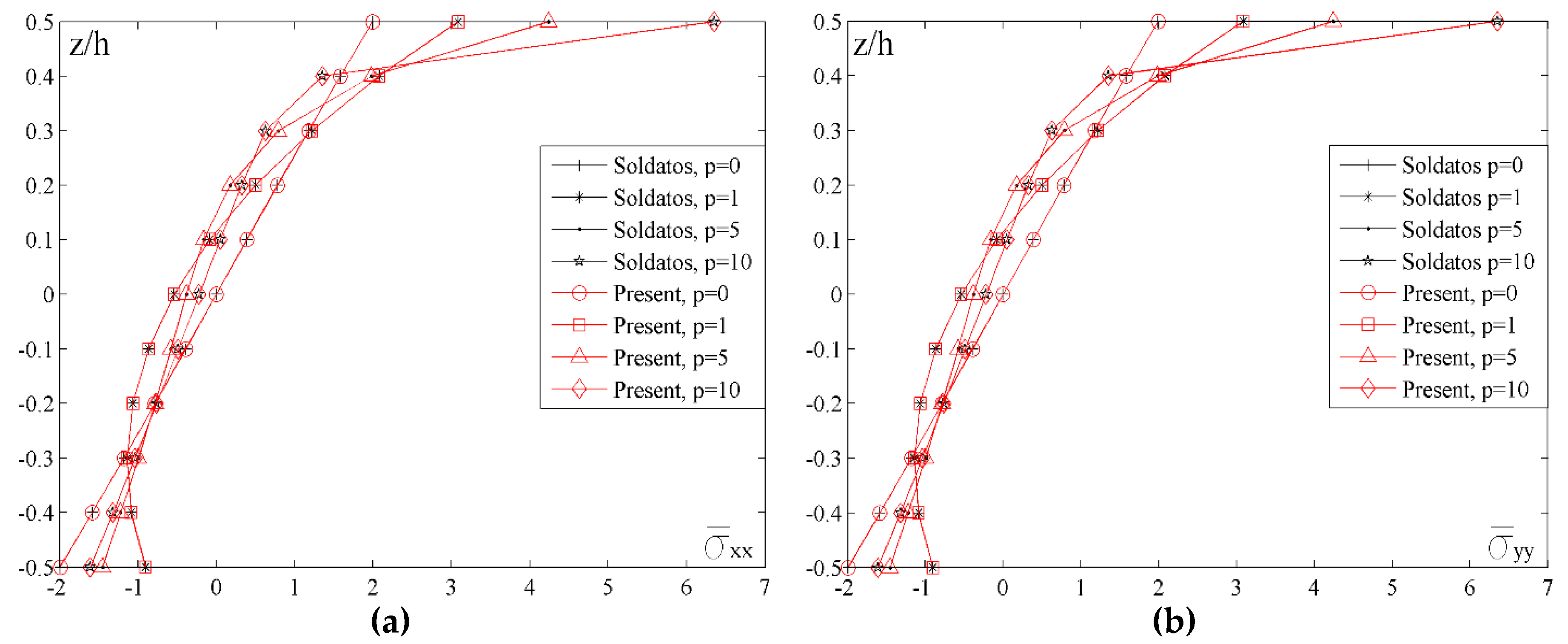
Figure 6 shows the distribution of normal stresses and across the thickness of the plate for different values of the index p. By analyzing the diagrams, it could be noticed that the curves representing both stresses are identical. Also, the basic property of FGM could be noticed, namely, the shift of a neutral plane in relation to the plane z/h = 0. It can also be seen that for the planes at the height z/h = 0.1–0.15 (depending on the chosen value of the index p) normal stresses have a positive sign which clearly indicates extension, and then they change the sign. In case when p = 0, (homogenous material made of ceramics) stress distribution is a familiar linear function with the neutral plane when z/h = 0. Maximum values of normal stresses due to compression are on the lower edge of the plate while the maximum values of normal stresses due to extension are on the upper edge of the plate. It could be noticed that with the increase of the index p value, maximum values of stresses due to extension are significantly increased.
Figure 7 shows the distribution of the shear stress across the thickness of the plate for different values of the index p (Figure 7a) and for different shape functions (Figure 7b), but for the unchanging values of a/h = 10 and a/b = 1. While analyzing the diagrams, it should be considered that when p = 0 the plate is homogenous made of ceramics, when p = 20 the plate is homogenous made of metal, and when 0 < p < 20 the plate is made of FGM. By analyzing the diagram in the Figure 7a, it could be noticed that for all values of the index p, the stress achieves the maximum value on the upper edge of the plate. Ceramic plate has the lowest maximum value. Therefore, with an increase of the metal volume fraction when p = 1, maximum stress value also increases and the highest value is achieved when the plate is homogenous made of metal. Moreover, apart from affecting the maximum stress values, the variation of the index p value also affects the shape of the stress distribution curve across the thickness of the plate.
In order to conduct a comparative analysis of the results for different shape functions and to estimate the application of the new shape function to the given problems, Figure 7b shows the distribution of the shear stress by using newly developed shape function and the shape functions given in Table 1. It is clearly seen that all the previously mentioned shape functions give identical results to the results obtained with the new shape function.
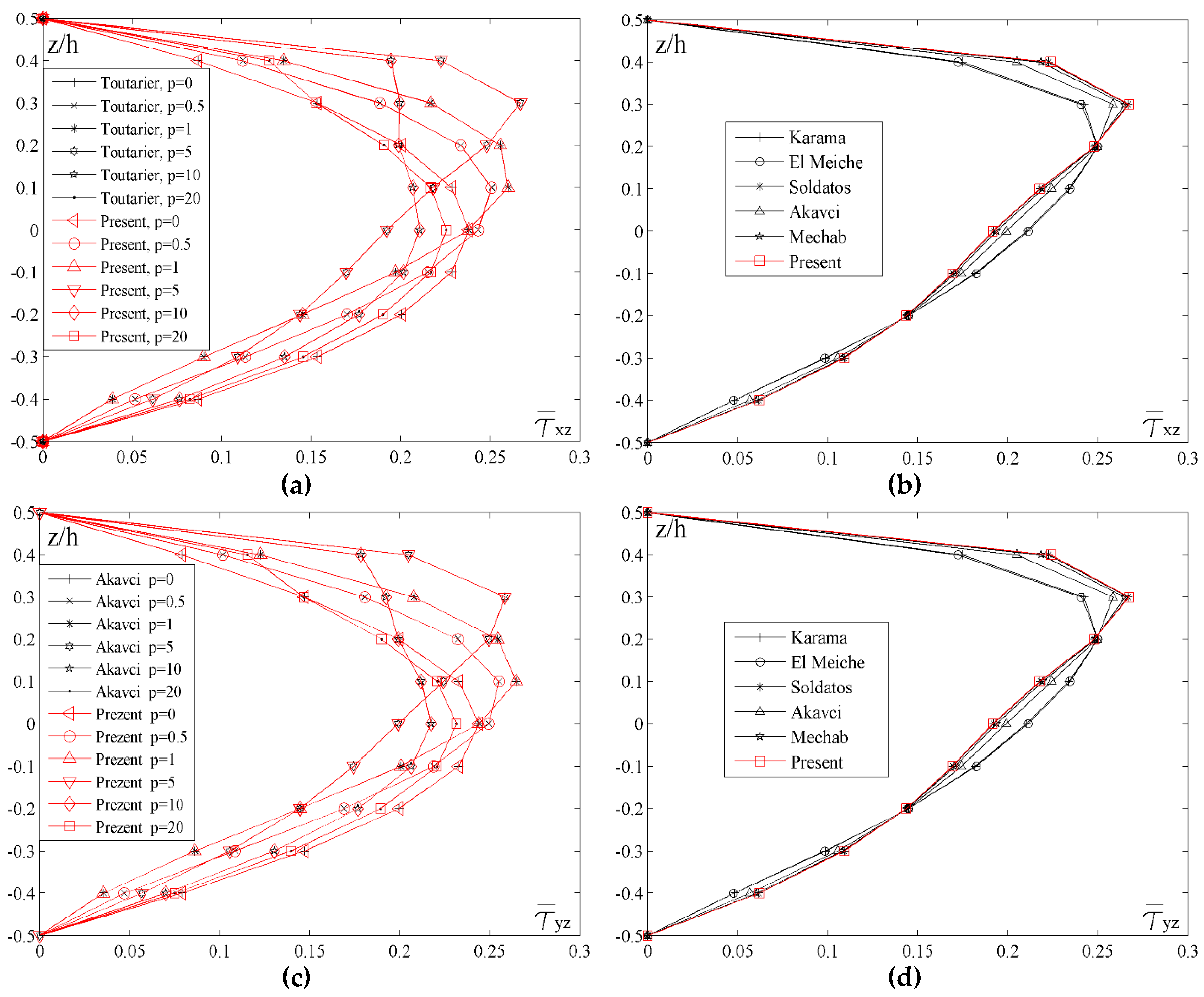
Figure 8 shows the distribution of transverse shear stresses and across the thickness of the plate for different values of the index p and for different shape functions. By analyzing transverse shear stresses in Figure 8a,c, a basic distinction between homogenous and FGM plates can be noticed. When plates are made of ceramics (p = 0) or metal (p = 20), it can be noticed that both stresses achieve maximum values in the plane at the height z/h = 0, due to the homogeneity of the material. On the other hand, when FGM plates are considered, there is an asymmetry in relation to the plane z/h = 0, therefore, when p = 1 stresses achieve maximum values in the plane z/h = 0.15, and when p = 5 stresses achieve maximum values when z/h = 0.3. In contrast to the homogenous ceramic plate, where stress distribution curve is a parabola with the maximum value in the plane z/h = 0, plates with the larger volume fraction of metal (p = 10) also achieve the maximum value of stress when z/h = 0, but the distribution curve is not a parabola. With the further increase of the metal volume fraction (p = 20), and although the plate can be practically considered homogenous, the diagram still shows the curve which is not a parabola. Generally, due to insignificant but still present ceramic fractions in the upper part of the plate, there is a slight deformity of the curve.
By conducting comparative analysis of the stresses and for different shape functions, and with fixed values of a/h = 10, a/b = 1 and p = 5, it could be seen in Figure 8b,d that, unlike the stress , the results do not match for all the shape functions. The most significant deviation could be noticed in the results for the El Meiche’s and Karama’s shape functions. The Akavci’s function also shows a slight deviation and it achieves maximum stress value at the height z/h = 0.25, while the results for all the other shape functions are almost identical, achieving the maximum stress value in the plane z/h = 0.25.
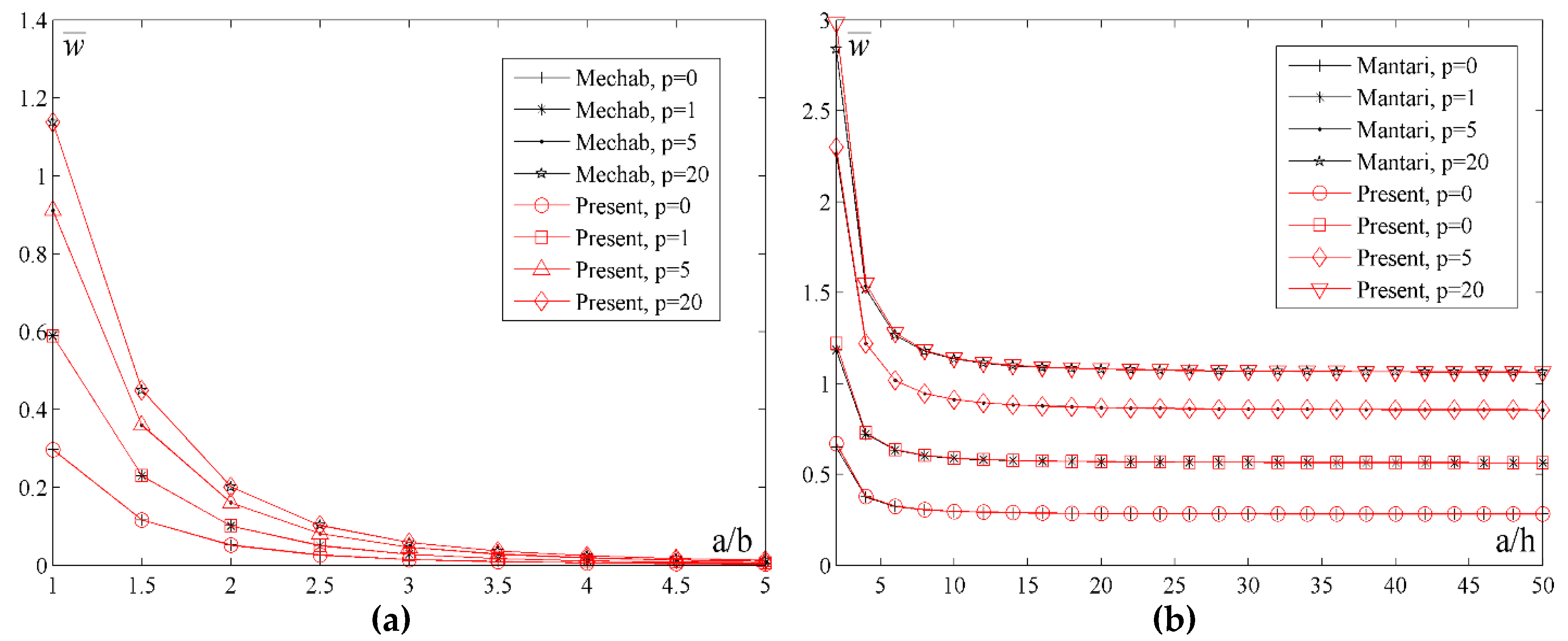
In order to understand the effects of increasing the index p as well as the effect of the thickness and geometry, Figure 9 shows the diagram of the normalized values of the displacement for different a/h and a/b ratios and values of the index p. By analyzing Figure 9a,b, it could be noticed that the displacement values for the metal plate (p = 20) are the highest, for the ceramic plate they are the lowest, and for the FGM plate they are somewhere in between. Moreover, by varying the volume fraction of metal or ceramics, a desired bending rigidity of the plate could be achieved. In Figure 9a, it could be seen that the curves gradually become closer when a/b > 4. In contrast to that, Figure 9b shows that with an increase of the ratio a/h the curves do not become closer, namely, the difference of the displacement ratio remains constant regardless of the index p change. This conclusion comes from the fact that in thin plates it is less possible to vary the volume fraction of the FGM constituents in the thickness direction of the plate and, thus, the index p has no effects.
In order to determine the effect of the elastic foundation on the displacements and stresses of the FGM plate, the results of different combinations of the FGM constituents have been presented, as well as different combinations of the Winkler (k0) and Pasternak (k1) coefficient of the elastic foundation. Apart from the normalization given in (26), it is necessary to apply the normalization of the coefficients k0 and k1, in the following form:
where the bending stiffness of the plate is .
The Table 4 and Table 5 show the results of the normalized values of displacements and stresses of the square plate on elastic foundation for p = 5, and p = 10, different values of k0 and k1 coefficients, as well as for two different ratios length/thickness of the plate (a/h = 10 and a/h = 5). In order to determine the effect of the elastic foundation on the displacements and stresses of the plate, the values of displacements and stresses for k0 = 0 and k1 = 0 are first shown, which practically matches the case of the plate without the elastic foundation. Afterwards, the values of the given coefficients are varied in order to conclude which of the two has greater influence. Based on the results, it is concluded that the introduction of the coefficient k0 has less influence on the change of the displacements and stresses values then when only k1 coefficient is introduced. By introducing k0 and k1 coefficients, bending stiffness of the plate increases, i.e., displacement and stresses values decrease and the influence of the Winkler coefficient is smaller than the influence of the Pasternak coefficient. This phenomenon is especially noticeable in the diagram dependency which is to be shown later.
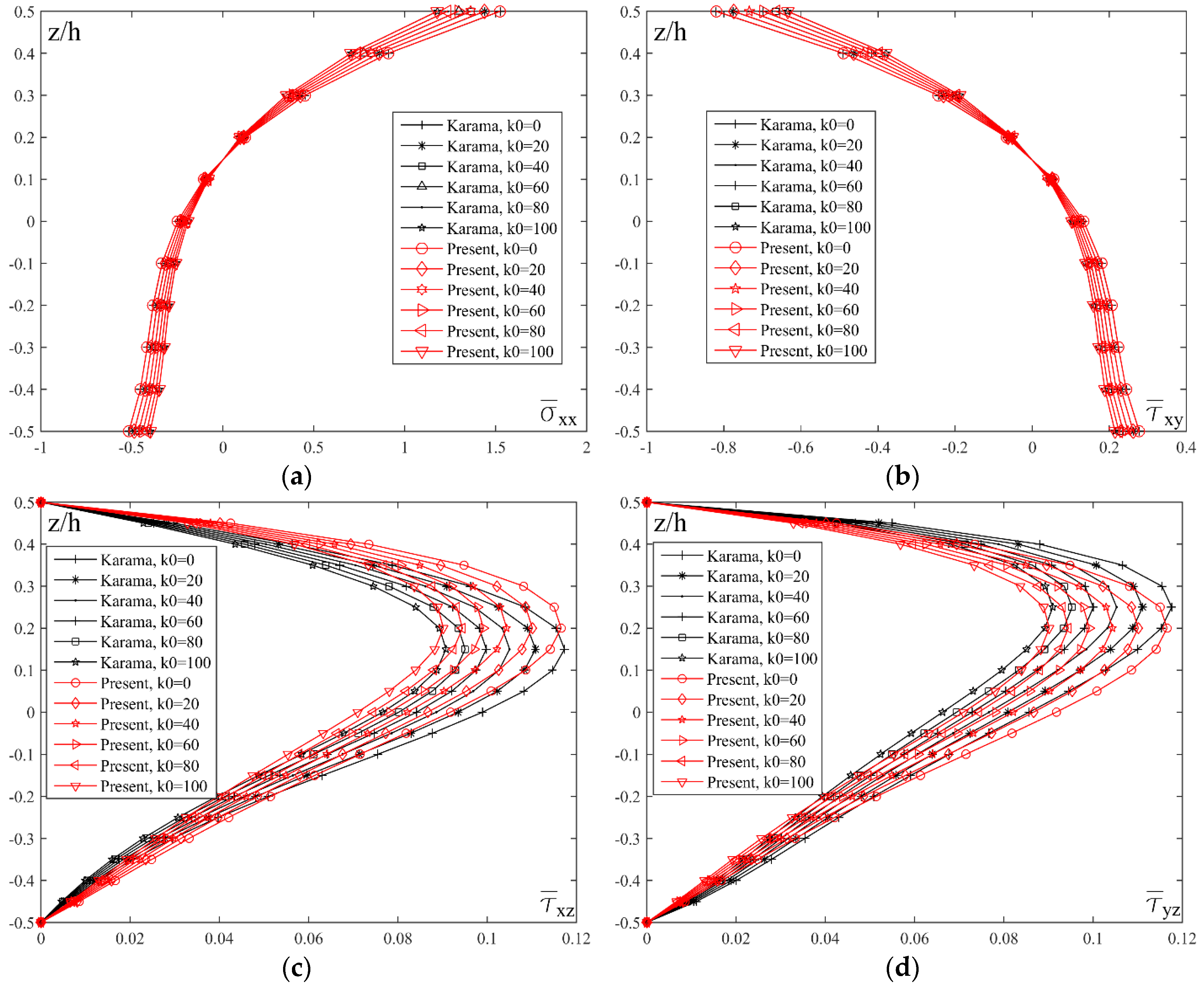
Figure 10 shows the effect of the Winkler coefficient k0 on the distribution of the normal stress , shear stress and transversal shear stresses and across the thickness of the plate on the elastic foundation. By analyzing the diagram, it can be seen that the value of the stresses and equals zero for z/h = 0.15. On the other hand, the maximum values of and stresses are at z/h = 0.2 when the new proposed shape function is applied, while the maximum values of mentioned stresses is respectively at z/h = 0.15 i.e., z/h = 0.25 for Karama’s shape function.
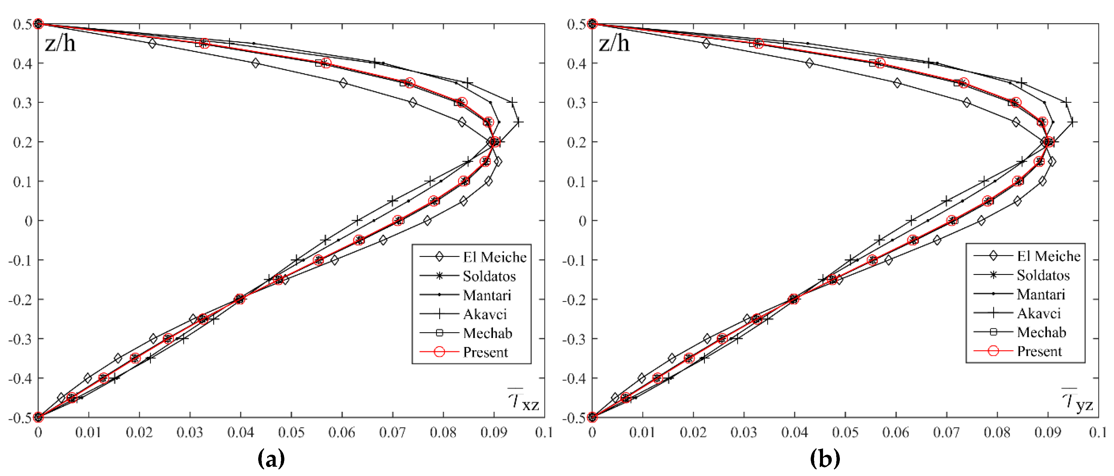
Figure 11 shows a comparative review of shear transversal stresses and distribution across the thickness of the plate on elastic foundation for different shape functions. As in the case of bending the plate without the elastic foundation, the shape functions do not give the same results. Therefore, it can be seen that for the Mantari’s and Akavci’s shape functions, stresses achieve their maximum values in the plane z/h = 0.25, and for El Meiche’s function in the plane z/h = 0.15, while for all the other shape functions as well as new proposed function, maximum values of the stresses are in the plane z/h = 0.2.
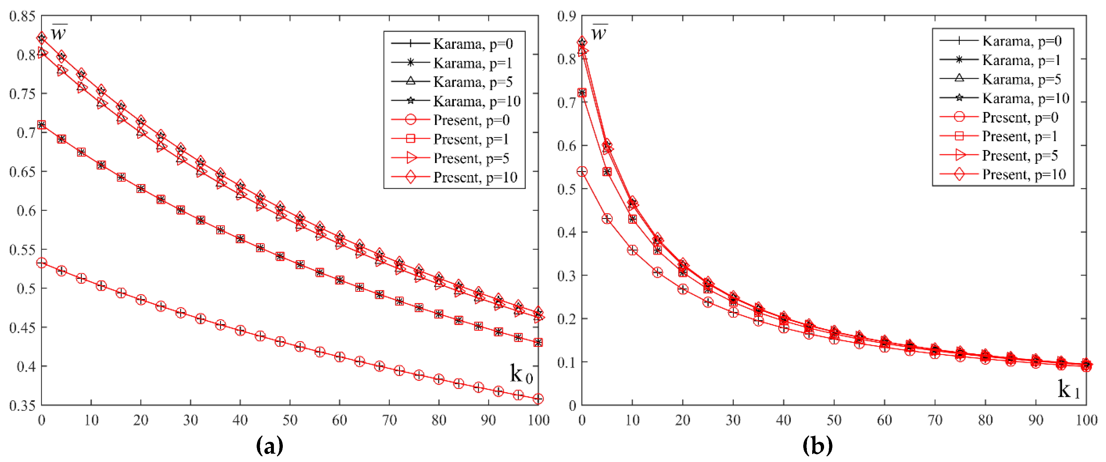
In order to get a clear insight on the effect of Winkler and Pasternak coefficients of the elastic foundation, Figure 12 shows the diagram of the normalized values of the displacement plate on the elastic foundation for different values of the index p and coefficients k0 and k1. By comparing the two diagrams, it can be seen that the change of the displacement value is higher with the increase of the coefficient k1 value than with the increase of the coefficient k0. For example, for the FGM plate when p = 5, and the increase of the coefficient from k0 = 0 to k0 = 100, the value of deflection changes twice its value. In the other case, with the change of the coefficient from k1 = 0 to k1 = 100, the value of deflection changes 8 times its value.
7. Conclusions
The results obtained in the previously published papers have been a starting point for developing and applying the new shape function. They have emphasized the importance and topicality of the research on the application of the functionally graded materials. A thorough and comprehensive systematization and investigation of the literature on the matter have been conducted according to the problem type which authors tried to solve during FGM plate analysis. Special attention and focus have been given to different deformation theories which authors had used in their analyses. The new shape function has been presented along with the comparative review of it with 13 different shape functions which were primarily developed by different authors for the analysis of composite laminates but, in this paper, they have been adjusted and implemented in appropriate relations for the analysis of FGM plates. Based on the obtained results of the static analysis of moderately thick and thick plates, it can be concluded that the newly developed shape function could be applied in the analysis of FGM plates.
By analyzing the obtained results, the following could be concluded:
- the values of the vertical displacement (deflection) and the corresponding stresses, which were obtained in this paper by using HSDT theory based on the new shape function, match the results of the same values obtained in the reference papers by using TSDT theory [58], quasi 3D theory of elasticity [59] and HSDT theories based on 13 different shape functions. However, in contrast to that, there are significant deviations of the results obtained for the values of the vertical displacement, especially for stresses , from the results obtained by CPT theory from the reference papers [60].
- the diagram of the distribution of transverse shear stresses and across the thickness of the plate shows the difference in behavior between a homogenous, ceramic or metal, plate and FGM plate. A basic property of FGM can be clearly seen, and that is the asymmetry of the stress distribution in relation to the middle plane of the plate (z = 0). The maximum values of stresses, depending on the volume fraction of certain constituents, are shifted in relation to the plane z=0, which represents a neutral plane in homogenous plates.
- the highest values of the displacement are obtained in a metal plate, the lowest in a ceramic plate and in an FGM plate, the values are somewhere in between and they depend on the volume fraction of the constituents. Based on that, it can be concluded that by varying the volume fraction of metal and ceramic, a desired bending rigidity of the plate can be achieved.
- a comparative analysis of the change of transverse shear stresses and across the thickness of the plate shows that, unlike the stress , their values do not match for all the shape functions.
- by introducing FG plate on Winkler–Pasternak model of elastic foundation is shown that the influence of the Winkler coefficient (k0) is smaller than the influence of the Pasternak coefficient (k1).
Author Contributions
D.Č. and G.B. proposed studied problem and applied solving method; A.R. and M.M. conducted the theoretical derivation; H.R. and D.D. conceived and performed the numerical examples; D.Č. and A.R. analyzed the results and wrote the manuscript.
Funding
This research received no external funding.
Acknowledgments
Research presented in this paper was supported by Ministry of Education, Science and Technological Development of Republic of Serbia, TR32036, TR33015 and multidisciplinary project III 44007.
Conflicts of Interest
The authors declare no conflict of interest.
References
- Golak, S.; Dolata, A.J. Fabrication of functionally graded composites using a homogenised low-frequency electromagnetic field. J. Compos. Mater. 2016, 50, 1751–1760. [Google Scholar] [CrossRef]
- Watanabe, Y.; Inaguma, Y.; Sato, H.; Miura-Fujiwara, E. A Novel Fabrication Method for Functionally Graded Materials under Centrifugal Force: The Centrifugal Mixed-Powder Method. Materials 2009, 2, 2510–2525. [Google Scholar] [CrossRef] [Green Version]
- El-Hadad, S.; Sato, H.; Miura-Fujiwara, E.; Watanabe, Y. Fabrication of Al-Al3Ti/Ti3Al Functionally Graded Materials under a Centrifugal Force. Materials 2010, 3, 4639–4656. [Google Scholar] [CrossRef] [PubMed]
- Jha, D.K.; Kant, T.; Singh, R.K. A critical review of recent research on functionally graded plates. Compos. Struct. 2013, 96, 833–849. [Google Scholar] [CrossRef]
- Bharti, I.; Gupta, N.; Gupta, K.M. Novel Applications of Functionally Graded Nano, Optoelectronic and Thermoelectric Materials. IJMMM Int. J. Mater. Mech. Manuf. 2013, 1, 221–224. [Google Scholar] [CrossRef]
- Saiyathibrahim, A.; Nazirudeen, M.S.S.; Dhanapal, P. Processing Techniques of Functionally Graded Materials—A Review. In Proceedings of the International Conference on Systems, Science, Control, Communication, Engineering and Technology 2015, Coimbatore, India, 10–11 August 2015. [Google Scholar]
- Birman, V.; Byrd, L.W. Modeling and analysis of functionally graded materials and structures. Appl. Mech. Rev. 2007, 60, 195–216. [Google Scholar] [CrossRef]
- Akbarzadeh, A.H.; Abedini, A.; Chen, Z.T. Effect of micromechanical models on structural responses of functionally graded plates. Compos. Struct. 2015, 119, 598–609. [Google Scholar] [CrossRef]
- Kirchhoff, G. Uber das gleichgewicht und die bewegung einer elastischen scheibe. J. Die Reine Angew. Math. 1850, 1850, 51–88. [Google Scholar] [CrossRef]
- Mindlin, R.D. Influence of rotatory inertia and shear on flexural motions of isotropic, elastic plates. J. Appl. Mech. 1951, 18, 31–38. [Google Scholar]
- Reissner, E. On bending of elastic plates. Q. Appl. Math. 1947, 5, 55–68. [Google Scholar] [CrossRef] [Green Version]
- Reissner, E. The effect of transverse shear deformation on the bending of elastic plates. J. Appl. Mech. 1945, 12, 69–72. [Google Scholar]
- Zenkour, A.M. An exact solution for the bending of thin rectangular plates with uniform, linear, and quadratic thickness variations. Int. J. Mech. Sci. 2003, 45, 295–315. [Google Scholar] [CrossRef]
- Mohammadi, M.; Saidi, A.R.; Jomehzadeh, E. Levy solution for buckling analysis of functionally graded rectangular plates. Appl. Compos. Mater. 2010, 17, 81–93. [Google Scholar] [CrossRef]
- Bhandari, M.; Purohit, K. Static Response of Functionally Graded Material Plate under Transverse Load for Varying Aspect Ratio. Int. J. Met. 2014, 2014, 980563. [Google Scholar] [CrossRef]
- Yang, J.; Shen, H.S. Non-linear analysis of FGM plates under transverse and in plane loads. Int. J. Nonlinear Mech. 2003, 38, 467–482. [Google Scholar] [CrossRef]
- Alinia, M.M.; Ghannadpour, S.A.M. Nonlinear analysis of pressure loaded FGM plates. Compos. Struct. 2009, 88, 354–359. [Google Scholar]
- Liu, D.Y.; Wang, C.Y.; Chen, W.Q. Free vibration of FGM plates with in-plane material inhomogeneity. Compos. Struct. 2010, 92, 1047–1051. [Google Scholar] [CrossRef]
- Ruan, M.; Wang, Z.M. Transverse vibrations of moving skew plates made of functionally graded material. J. Vib. Control 2016, 22, 3504–3517. [Google Scholar] [CrossRef]
- Woo, J.; Meguid, S.A.; Ong, L.S. Nonlinear free vibration behavior of functionally graded plates. J. Sound Vib. 2006, 289, 595–611. [Google Scholar] [CrossRef]
- Hu, Y.; Zhang, X. Parametric vibrations and stability of a functionally graded plate. Mech. Based Des. Struct. 2011, 39, 367–377. [Google Scholar]
- Taczała, M.; Buczkowski, R.; Kleiber, M. Nonlinear free vibration of pre- and post-buckled FGM plates on two-parameter foundation in the thermal environment. Compos. Struct. 2016, 137, 85–92. [Google Scholar] [CrossRef]
- Xing, C.; Wang, Y.; Waisman, H. Fracture analysis of cracked thin-walled structures using a high-order XFEM and Irwin’s integral. Comput. Struct. 2019, 212, 1–19. [Google Scholar] [CrossRef]
- Kim, K.D.; Lomboy, G.R.; Han, S.C. Geometrically non-linear analysis of functionally graded material (FGM) plates and shells using a four-node quasi-conforming shell element. J. Compos. Mater. 2008, 42, 485–511. [Google Scholar] [CrossRef]
- Wu, T.L.; Shukla, K.K.; Huang, J.H. Nonlinear static and dynamic analysis of functionally graded plates. IJAME Int. J. Appl. Mech. Eng. 2006, 11, 679–698. [Google Scholar]
- Reddy, J.N. A simple higher-order theory for laminated composite plates. J. Appl. Mech. 1984, 51, 745–752. [Google Scholar] [CrossRef]
- Phan, N.D.; Reddy, J.N. Analysis of laminated composite plates using a higher-order shear deformation theory. Int. Numer. Methods Eng. 1985, 21, 2201–2219. [Google Scholar] [CrossRef]
- Reddy, J.N. Analysis of functionally graded plates. Int. Numer. Methods Eng. 2000, 47, 663–684. [Google Scholar] [CrossRef]
- Kim, J.; Reddy, J.N. A general third-order theory of functionally graded plates with modified couple stress effect and the von Kármán nonlinearity: Theory and finite element analysis. Acta Mech. 2015, 226, 2973–2998. [Google Scholar] [CrossRef]
- Dung, D.V.; Nga, N.T. Buckling and postbuckling nonlinear analysis of imperfect FGM plates reinforced by FGM stiffeners with temperature-dependent properties based on TSDT. Acta Mech. 2016, 227, 2377–2401. [Google Scholar] [CrossRef]
- Bodaghi, M.; Saidi, A.R. Thermoelastic buckling behavior of thick functionally graded rectangular plates. Arch. Appl. Mech. 2011, 81, 1555–1572. [Google Scholar] [CrossRef]
- Yang, J.; Liew, K.M.; Kitipornchai, S. Dynamic stability of laminated FGM plates based on higher-order shear deformation theory. Comput. Mech. 2004, 33, 305–315. [Google Scholar] [CrossRef]
- Akbarzadeh, A.H.; Zad, S.H.; Eslami, M.R.; Sadighi, M. Mechanical behaviour of functionally graded plates under static and dynamic loading. Proc. Inst. Mech. Eng. Part C J. Mech. Eng. Sci. 2011, 225, 326–333. [Google Scholar] [CrossRef]
- Thai, H.T.; Choi, D.H. Efficient higher-order shear deformation theories for bending and free vibration analyses of functionally graded plates. Arch. Appl. Mech. 2013, 83, 1755–1771. [Google Scholar] [CrossRef]
- Thai, H.T.; Park, T.; Choi, D.H. An efficient shear deformation theory for vibration of functionally graded plates. Arch. Appl. Mech. 2013, 83, 137–149. [Google Scholar]
- Lo, K.H.; Christensen, R.M.; Wu, E.M. A high-order theory of plate deformation part 1: Homogeneous plates. J. Appl. Mech. 1977, 44, 663–668. [Google Scholar] [CrossRef]
- Lo, K.H.; Christensen, R.M.; Wu, E.M. A high-order theory of plate deformation part 2: Laminated plates. J. Appl. Mech. 1977, 44, 669–676. [Google Scholar] [CrossRef]
- Kant, T.; Swaminathan, K. Analytical solutions for free vibration of laminated composite and sandwich plates based on a higher-order refined theory. Compos. Struct. 2001, 53, 73–85. [Google Scholar] [CrossRef] [Green Version]
- Kant, T.; Swaminathan, K. Analytical solutions for the static analysis of laminated composite and sandwich plates based on a higher order refined theory. Compos. Struct. 2002, 56, 329–344. [Google Scholar] [CrossRef] [Green Version]
- Xiang, S.; Kang, G.; Xing, B. A nth-order shear deformation theory for the free vibration analysis on the isotropic plates. Meccanica 2012, 47, 1913–1921. [Google Scholar] [CrossRef]
- Song, X.; Kang, G. A nth-order shear deformation theory for the bending analysis on the functionally graded plates. Eur. J. Mech. A-Solid 2013, 37, 336–343. [Google Scholar]
- Song, X.; Kang, G.; Liu, Y. A nth-order shear deformation theory for natural frequency of the functionally graded plates on elastic foundations. Compos. Struct. 2014, 11, 224–231. [Google Scholar]
- Soldatos, K. A transverse shear deformation theory for homogeneous monoclinic plates. Acta Mech. 1992, 94, 195–220. [Google Scholar] [CrossRef]
- Aydogdu, M. A new shear deformation theory for laminated composite plates. Compos. Struct. 2009, 89, 94–101. [Google Scholar] [CrossRef]
- Mantari, J.L.; Oktem, A.S.; Soares, S.G. A new trigonometric shear deformation theory for isotropic, laminated composite and sandwich plates. Int. J. Solids Struct. 2012, 49, 43–53. [Google Scholar] [CrossRef]
- Mantari, J.L.; Bonilla, E.M.; Soares, C.G. A new tangential-exponential higher order shear deformation theory for advanced composite plates. Compos. Part B-Eng. 2014, 60, 319–328. [Google Scholar] [CrossRef]
- El Meichea, N.; Tounsia, A.; Zianea, N.; Mechaba, I.; El Abbes, A.B. A new hyperbolic shear deformation theory for buckling and vibration of functionally graded sandwich plate. Int. J. Mech. Sci. 2011, 53, 237–247. [Google Scholar] [CrossRef]
- Mechab, B.; Mechab, I.; Benaissa, S. Analysis of thick orthotropic laminated composite plates based on higher order shear deformation theory by the new function under thermo-mechanical loading. Compos. Part B-Eng. 2014, 43, 1453–1458. [Google Scholar] [CrossRef]
- Akavci, S.S. Two new hyperbolic shear displacement models for orthotropic laminated composite plates. Mech. Compos. Mater. 2010, 46, 215–226. [Google Scholar] [CrossRef]
- Viola, E.; Tornabene, F.; Fantuzzi, N. General higher-order shear deformation theories for the free vibration analysis of completely doubly-curved laminated shells and panels. Compos. Struct. 2013, 95, 639–666. [Google Scholar] [CrossRef]
- Grover, N.; Maiti, D.K.; Singh, B.N. Flexural behavior of general laminated composite and sandwich plates using a secant function based shear deformation theory. Lat. Am. J. Solids Strut. 2014, 11, 1275–1297. [Google Scholar] [CrossRef] [Green Version]
- Ambartsumyan, A.S. On the Theory of Anisotropic Shells and Plates. In Proceedings of the Non-Homogeneity in Elasticity and Plasticity: Symposium, Warsaw, Poland, 2–9 September 1958; Olszak, W., Ed.; Pergamon Press: London, UK, 1958. [Google Scholar]
- Reissner, E.; Stavsky, Y. Bending and Stretching of Certain Types of Heterogeneous Aeolotropic Elastic Plates. J. Appl. Mech. 1961, 28, 402–408. [Google Scholar] [CrossRef]
- Stein, M. Nonlinear theory for plates and shells including the effects of transverse shearing. AIAA J. 1986, 24, 1537–1544. [Google Scholar] [CrossRef]
- Mantari, J.L.; Oktem, A.S.; Soares, G.C. Bending and free vibration analysis of isotropic and multilayered plates and shells by using a new accurate higherorder shear deformation theory. Compos. Part B-Eng. 2012, 43, 3348–3360. [Google Scholar] [CrossRef]
- Karama, M.; Afaq, K.S.; Mistou, S. Mechanical behaviour of laminated composite beam by the new multi-layered laminated composite structures model with transverse shear stress continuity. Int. J. Solids Struct. 2003, 40, 1525–1546. [Google Scholar] [CrossRef]
- Reddy, J.N. Mechanics of Laminated Composite Plates and Shells: Theory and Analysis; CRC Press LLC: New York, NY, USA, 2004. [Google Scholar]
- Wu, C.P.; Li, H.Y. An RMVT-based third-order shear deformation theory of multilayered functionally graded material plates. Compos. Struct. 2010, 92, 2591–2605. [Google Scholar]
- Wu, C.P.; Chiu, K.H.; Wang, Y.M. RMVT-based meshless collocation and element-free Galerkin methods for the quasi-3D analysis of multilayered composite and FGM plates. Compos. Struct. 2011, 93, 923–943. [Google Scholar] [CrossRef]
- Carrera, E.; Brischetto, S.; Robaldo, A. Variable kinematic model for the analysis of functionally graded material plates. AIAA J. 2008, 46, 194–203. [Google Scholar] [CrossRef]
Figure 1.
Schematic of continuously graded microstructure with metal-ceramic constituents: (a) smoothly graded microstructure; (b) enlarged view; (c) ceramic-metal functionally graded materials (FGM).
Figure 1.
Schematic of continuously graded microstructure with metal-ceramic constituents: (a) smoothly graded microstructure; (b) enlarged view; (c) ceramic-metal functionally graded materials (FGM).

Figure 2.
Different types of functionally graded materials based on nature of gradients: (а) fraction gradient type; (b) shape gradient type; (c) orientation gradient type; (d) size gradient type.
Figure 2.
Different types of functionally graded materials based on nature of gradients: (а) fraction gradient type; (b) shape gradient type; (c) orientation gradient type; (d) size gradient type.

Figure 3.
Geometry of the plate: (a) FGM plate; (b) FGM plate on elastic foundation.

Figure 4.
The comparison of homogenous plates (ceramic or metal) and FGM plates: (a) volume fraction of the material; (b) homogenous and FGM plates.
Figure 4.
The comparison of homogenous plates (ceramic or metal) and FGM plates: (a) volume fraction of the material; (b) homogenous and FGM plates.

Figure 5.
Shape function diagrams: (a) shape function from literature; (b) new proposed shape function.
Figure 5.
Shape function diagrams: (a) shape function from literature; (b) new proposed shape function.

Figure 6.
Distribution of the normalized values of the normal stresses and across the thickness of the plate for different values of the index p: (a) a/h = 10, a/b = 1; (b) a/h = 10, a/b = 1.
Figure 6.
Distribution of the normalized values of the normal stresses and across the thickness of the plate for different values of the index p: (a) a/h = 10, a/b = 1; (b) a/h = 10, a/b = 1.

Figure 7.
Distribution of the normalized values of the shear stress across the thickness of the plate for different values of the index p and different shape function: (a) a/h = 10, a/b = 1; (b) a/h = 10, a/b = 1, p = 5.
Figure 7.
Distribution of the normalized values of the shear stress across the thickness of the plate for different values of the index p and different shape function: (a) a/h = 10, a/b = 1; (b) a/h = 10, a/b = 1, p = 5.

Figure 8.
Distribution of the normalized values of the transverse shear stresses and across the thickness of the plate for different values of the index p and different shape functions: (a) a/h = 10, a/b = 1; (b) a/h = 10, a/b = 1, p = 5; (c) a/h = 10, a/b = 1; (d) a/h = 10, a/b = 1, p = 5.
Figure 8.
Distribution of the normalized values of the transverse shear stresses and across the thickness of the plate for different values of the index p and different shape functions: (a) a/h = 10, a/b = 1; (b) a/h = 10, a/b = 1, p = 5; (c) a/h = 10, a/b = 1; (d) a/h = 10, a/b = 1, p = 5.

Figure 9.
Normalized values of the displacement for different a/h and a/b ratios and the values of the index p: (a) a/h = 10; (b) a/b = 1.
Figure 9.
Normalized values of the displacement for different a/h and a/b ratios and the values of the index p: (a) a/h = 10; (b) a/b = 1.

Figure 10.
Distribution of the normalized values of the normal stresses , the shear stress and the transverse shear stresses and across the thickness of the plate on elastic foundation for different values of the coefficients k0: (a) a/h = 10, a/b = 1, p = 2, k1 = 10; (b) a/h = 10, a/b = 1, p = 2, k1 = 10; (c) a/h = 10, a/b = 1, p = 2, k1 = 10; (d) a/h = 10, a/b = 1, p = 2, k1 = 10.

Figure 11.
Distribution of the normalized values of the transverse shear stresses and across the thickness of the plate on elastic foundation for different shape functions: (a) a/h = 10, a/b = 1, p = 2, k0 = 100, k1 = 10; (b) a/h = 10, a/b = 1, p = 2, k0 = 100, k1 = 10.
Figure 11.
Distribution of the normalized values of the transverse shear stresses and across the thickness of the plate on elastic foundation for different shape functions: (a) a/h = 10, a/b = 1, p = 2, k0 = 100, k1 = 10; (b) a/h = 10, a/b = 1, p = 2, k0 = 100, k1 = 10.

Figure 12.
Normalized values of the displacement of plate on elastic foundation for different values index p and coefficients k0 and k1: (a) a/h = 10, a/b = 0.2, k1 = 10; (b) a/h = 10, a/b = 0.2, k0 = 10.
Figure 12.
Normalized values of the displacement of plate on elastic foundation for different values index p and coefficients k0 and k1: (a) a/h = 10, a/b = 0.2, k1 = 10; (b) a/h = 10, a/b = 0.2, k0 = 10.


Table 1.
Shear deformation shape functions.
| Number of Shape Function (SF) | Names of Authors | Shape Function f(z) |
|---|---|---|
| SF 1 | Ambartsumain [52] | |
| SF 2 | Kaczkowski, Panc and Reissner [53] | |
| SF 3 | Levy, Stein, Touratier [54] | |
| SF 4 | Mantari at al. [55] | |
| SF 5–6 | Mantari at al. [45] | |
| SF 7 | Karama at al. [56], Aydogdu [44] | |
| SF 8 | Mantari at al. [46] | |
| SF 9 | El Meiche at al. [47] | |
| SF 10 | Soldatos [43] | |
| SF 11 | Akavci and Tanrikulu [49] | |
| SF 12 | Akavci and Tanrikulu [49] | |
| SF 13 | Mechab at al. [48] |
Table 2.
Material properties of FGM constituents.
| Material | Material Properties | |
|---|---|---|
| Elasticity Modulus, E[GPa] | Poisson’s Ratio, ν | |
| Aluminum (Al) | ||
| Alumina (Al2O3) | ||
Table 3.
Normalized values of displacement and stresses of square plate for different values of the index p and the ratio a/h (a/b = 1). CPT: classical plate theory; TSDT: third-order shear deformation theory.
Table 3.
Normalized values of displacement and stresses of square plate for different values of the index p and the ratio a/h (a/b = 1). CPT: classical plate theory; TSDT: third-order shear deformation theory.
| p | Theory | ||||||||
|---|---|---|---|---|---|---|---|---|---|
| a/b = 1 | |||||||||
| a/h = 10 | a/h = 5 | a/h = 10 | a/h = 5 | a/h = 10 | a/h = 5 | a/h = 10 | a/h = 5 | ||
| 1 | Present study | 0.5889 | 0.6687 | 1.4899 | 0.7345 | 0.6111 | 0.3034 | 0.2604 | 0.2599 |
| CPT [60] | 0.5623 | ----- | 2.0150 | ----- | ----- | ----- | ----- | ----- | |
| Quasi 3D [59] | 0.5876 | ----- | 1.5061 | ----- | 0.6112 | ----- | 0.2511 | ----- | |
| TSDT [58] | 0.5890 | ----- | 1.4898 | ----- | 0.6111 | ----- | 0.2599 | ----- | |
| SF 1 | 0.5889 | 0.6687 | 1.4898 | 0.7344 | 0.6111 | 0.3034 | 0.2607 | 0.2602 | |
| SF 2 | 0.5889 | 0.6687 | 1.4898 | 0.7344 | 0.6111 | 0.3034 | 0.2607 | 0.2602 | |
| SF 3 | 0.5889 | 0.6685 | 1.4894 | 0.7336 | 0.6110 | 0.3033 | 0.2621 | 0.2615 | |
| SF 4 | 0.5880 | 0.6648 | 1.4888 | 0.7323 | 0.6109 | 0.3030 | 0.2566 | 0.2554 | |
| SF 5 | 0.5889 | 0.6687 | 1.4898 | 0.7344 | 0.6111 | 0.3034 | 0.2607 | 0.2601 | |
| SF 6 | 0.5888 | 0.6683 | 1.4908 | 0.7363 | 0.6113 | 0.3038 | 0.2551 | 0.2547 | |
| SF 7 | 0.5887 | 0.6679 | 1.4891 | 0.7330 | 0.6109 | 0.3031 | 0.2624 | 0.2616 | |
| SF 8 | 0.5887 | 0.6679 | 1.4891 | 0.7330 | 0.6109 | 0.3031 | 0.2623 | 0.2615 | |
| SF 9 | 0.5887 | 0.6679 | 1.4891 | 0.7330 | 0.6109 | 0.3031 | 0.2623 | 0.2615 | |
| SF 10 | 0.5889 | 0.6687 | 1.4898 | 0.7344 | 0.6111 | 0.3034 | 0.2605 | 0.2600 | |
| SF 11 | 0.5887 | 0.6679 | 1.4902 | 0.7352 | 0.6112 | 0.3036 | 0.2569 | 0.2566 | |
| SF 12 | 0.5889 | 0.6686 | 1.4895 | 0.7338 | 0.6110 | 0.3033 | 0.2617 | 0.2611 | |
| SF 13 | 0.5889 | 0.6687 | 1.4898 | 0.7343 | 0.6111 | 0.3034 | 0.2609 | 0.2603 | |
| 2 | Present study | 0.7572 | 0.8670 | 1.3961 | 0.6838 | 0.5442 | 0.2696 | 0.2732 | 0.2726 |
| CPT [60] | ----- | ----- | ----- | ----- | ----- | ----- | ----- | ----- | |
| Quasi 3D [59] | 0.7571 | ----- | 1.4133 | ----- | 0.5436 | ----- | 0.2495 | ----- | |
| TSDT [58] | 0.7573 | ----- | 1.3960 | ----- | 0.5442 | ----- | 0.2721 | ----- | |
| SF 1 | 0.7573 | 0.8671 | 1.3960 | 0.6836 | 0.5442 | 0.2695 | 0.2736 | 0.2730 | |
| SF 2 | 0.7573 | 0.8671 | 1.3960 | 0.6836 | 0.5442 | 0.2695 | 0.2736 | 0.2730 | |
| SF 3 | 0.7573 | 0.8671 | 1.3954 | 0.6824 | 0.5440 | 0.2693 | 0.2763 | 0.2755 | |
| SF 4 | 0.7563 | 0.8629 | 1.3940 | 0.6797 | 0.5437 | 0.2687 | 0.2741 | 0.2726 | |
| SF 5 | 0.7572 | 0.8671 | 1.3961 | 0.6836 | 0.5442 | 0.2695 | 0.2735 | 0.2729 | |
| SF 6 | 0.7568 | 0.8656 | 1.3975 | 0.6865 | 0.5444 | 0.2701 | 0.2653 | 0.2649 | |
| SF 7 | 0.7572 | 0.8667 | 1.3949 | 0.6813 | 0.5439 | 0.2691 | 0.2777 | 0.2767 | |
| SF 8 | 0.7572 | 0.8666 | 1.3948 | 0.6812 | 0.5439 | 0.2691 | 0.2777 | 0.2768 | |
| SF 9 | 0.7572 | 0.8666 | 1.3948 | 0.6812 | 0.5439 | 0.2691 | 0.2777 | 0.2768 | |
| SF 10 | 0.7572 | 0.8670 | 1.3961 | 0.6837 | 0.5442 | 0.2696 | 0.2733 | 0.2727 | |
| SF 11 | 0.7567 | 0.8649 | 1.3969 | 0.6854 | 0.5444 | 0.2699 | 0.2667 | 0.2663 | |
| SF 12 | 0.7573 | 0.8672 | 1.3956 | 0.6827 | 0.5441 | 0.2694 | 0.2755 | 0.2748 | |
| SF 13 | 0.7573 | 0.8671 | 1.3960 | 0.6835 | 0.5442 | 0.2695 | 0.2739 | 0.2733 | |
| 4 | Present study | 0.8814 | 1.0406 | 1.1795 | 0.5707 | 0.5669 | 0.2799 | 0.2529 | 0.2523 |
| CPT [60] | 0.8281 | ----- | 1.6049 | ----- | ----- | ----- | ----- | ----- | |
| Quasi 3D [59] | 0.8823 | ----- | 1.1841 | ----- | 0.5671 | ----- | 0.2362 | ----- | |
| TSDT [58] | 0.8815 | ----- | 1.1794 | ----- | 0.5669 | ----- | 0.2519 | ----- | |
| SF 1 | 0.8814 | 1.0409 | 1.1794 | 0.5704 | 0.5669 | 0.2798 | 0.2537 | 0.2529 | |
| SF 2 | 0.8814 | 1.0409 | 1.1794 | 0.5704 | 0.5669 | 0.2798 | 0.2537 | 0.2529 | |
| SF 3 | 0.8818 | 1.0423 | 1.1783 | 0.5684 | 0.5667 | 0.2795 | 0.2580 | 0.2571 | |
| SF 4 | 0.8815 | 1.0402 | 1.1756 | 0.5630 | 0.5662 | 0.2784 | 0.2623 | 0.2606 | |
| SF 5 | 0.8814 | 1.0408 | 1.1794 | 0.5705 | 0.5669 | 0.2799 | 0.2535 | 0.2528 | |
| SF 6 | 0.8802 | 1.0360 | 1.1816 | 0.5749 | 0.5673 | 0.2807 | 0.2421 | 0.2417 | |
| SF 7 | 0.8820 | 1.0429 | 1.1774 | 0.5666 | 0.5665 | 0.2791 | 0.2612 | 0.2601 | |
| SF 8 | 0.8820 | 1.0429 | 1.1773 | 0.5664 | 0.5665 | 0.2791 | 0.2614 | 0.2603 | |
| SF 9 | 0.8820 | 1.0429 | 1.1773 | 0.5664 | 0.5665 | 0.2791 | 0.2614 | 0.2603 | |
| SF 10 | 0.8814 | 1.0407 | 1.1795 | 0.5706 | 0.5669 | 0.2799 | 0.2532 | 0.2525 | |
| SF 11 | 0.8798 | 1.0346 | 1.1811 | 0.5739 | 0.5672 | 0.2805 | 0.2427 | 0.2423 | |
| SF 12 | 0.8817 | 1.0420 | 1.1786 | 0.5690 | 0.5668 | 0.2796 | 0.2568 | 0.2559 | |
| SF 13 | 0.8815 | 1.0411 | 1.1793 | 0.5702 | 0.5669 | 0.2798 | 0.2541 | 0.2534 | |
| 8 | Present study | 0.9745 | 1.1828 | 0.9478 | 0.4544 | 0.5858 | 0.2886 | 0.2082 | 0.2076 |
| CPT [60] | ----- | ----- | ----- | ----- | ----- | ----- | ----- | ----- | |
| Quasi 3D [59] | 0.9739 | ----- | 0.9622 | ----- | 0.5883 | ----- | 0.2261 | ----- | |
| TSDT [58] | 0.9747 | ----- | 0.9747 | ----- | 0.5858 | ----- | 0.2087 | ----- | |
| SF 1 | 0.9746 | 1.1832 | 0.9476 | 0.4541 | 0.5858 | 0.2886 | 0.2087 | 0.2081 | |
| SF 2 | 0.9746 | 1.1832 | 0.9476 | 0.4541 | 0.5858 | 0.2886 | 0.2087 | 0.2081 | |
| SF 3 | 0.9749 | 1.1845 | 0.9465 | 0.4520 | 0.5856 | 0.2881 | 0.2120 | 0.2113 | |
| SF 4 | 0.9739 | 1.1794 | 0.9435 | 0.4461 | 0.5850 | 0.2871 | 0.2139 | 0.2125 | |
| SF 5 | 0.9745 | 1.1831 | 0.9477 | 0.4542 | 0.5858 | 0.2886 | 0.2086 | 0.2080 | |
| SF 6 | 0.9730 | 1.1774 | 0.9500 | 0.4589 | 0.5863 | 0.2895 | 0.1995 | 0.1991 | |
| SF 7 | 0.9751 | 1.1848 | 0.9455 | 0.4500 | 0.5854 | 0.2877 | 0.2143 | 0.2134 | |
| SF 8 | 0.9751 | 1.1848 | 0.9454 | 0.4498 | 0.5854 | 0.2877 | 0.2145 | 0.2135 | |
| SF 9 | 0.9751 | 1.1848 | 0.9454 | 0.4498 | 0.5854 | 0.2877 | 0.2145 | 0.2135 | |
| SF 10 | 0.9745 | 1.1830 | 0.9477 | 0.4543 | 0.5858 | 0.2886 | 0.2084 | 0.2078 | |
| SF 11 | 0.9727 | 1.1763 | 0.9496 | 0.4581 | 0.5861 | 0.2893 | 0.2006 | 0.2003 | |
| SF 12 | 0.9749 | 1.1842 | 0.9469 | 0.4526 | 0.5856 | 0.2883 | 0.2111 | 0.2104 | |
| SF 13 | 0.9746 | 1.1833 | 0.9475 | 0.4539 | 0.5858 | 0.2885 | 0.2091 | 0.2084 | |
| 20 | Present study | 1.1377 | 1.3727 | 0.7710 | 0.3721 | 0.6079 | 0.2993 | 0.2011 | 0.2005 |
| CPT [60] | ----- | ----- | ----- | ----- | ----- | ----- | ----- | ----- | |
| Quasi 3D [59] | ----- | ----- | ----- | ----- | ----- | ----- | ----- | ----- | |
| TSDT [58] | ----- | ----- | ----- | ----- | ----- | ----- | ----- | ----- | |
| SF 1 | 1.1377 | 1.3727 | 0.7709 | 0.3720 | 0.6078 | 0.2993 | 0.2013 | 0.2008 | |
| SF 2 | 1.1377 | 1.3727 | 0.7709 | 0.3720 | 0.6078 | 0.2993 | 0.2013 | 0.2008 | |
| SF 3 | 1.1374 | 1.3712 | 0.7702 | 0.3707 | 0.6076 | 0.2989 | 0.2025 | 0.2019 | |
| SF 4 | 1.1338 | 1.3561 | 0.7687 | 0.3677 | 0.6073 | 0.2982 | 0.1979 | 0.1966 | |
| SF 5 | 1.1377 | 1.3727 | 0.7709 | 0.3720 | 0.6078 | 0.2993 | 0.2013 | 0.2007 | |
| SF 6 | 1.1375 | 1.3723 | 0.7723 | 0.3748 | 0.6083 | 0.3002 | 0.1963 | 0.1960 | |
| SF 7 | 1.1368 | 1.3686 | 0.7697 | 0.3696 | 0.6075 | 0.2986 | 0.2028 | 0.2019 | |
| SF 8 | 1.1367 | 1.3683 | 0.7696 | 0.3695 | 0.6075 | 0.2986 | 0.2027 | 0.2019 | |
| SF 9 | 1.1367 | 1.3683 | 0.7696 | 0.3695 | 0.6075 | 0.2986 | 0.2027 | 0.2019 | |
| SF 10 | 1.1377 | 1.3727 | 0.7709 | 0.3721 | 0.6079 | 0.2993 | 0.2012 | 0.2006 | |
| SF 11 | 1.1375 | 1.3722 | 0.7720 | 0.3741 | 0.6081 | 0.2998 | 0.1983 | 0.1979 | |
| SF 12 | 1.1375 | 1.3718 | 0.7704 | 0.3711 | 0.6077 | 0.2990 | 0.2022 | 0.2016 | |
| SF 13 | 1.1377 | 1.3726 | 0.7708 | 0.3718 | 0.6078 | 0.2993 | 0.2015 | 0.2009 | |
Table 4.
Normalized values of displacement and stresses of square plate on elastic foundation for p = 5, different values of the k0 и k1 and the ratio a/h (a/b = 1).
Table 4.
Normalized values of displacement and stresses of square plate on elastic foundation for p = 5, different values of the k0 и k1 and the ratio a/h (a/b = 1).
| p | k0 | k1 | Theory | ||||||||
|---|---|---|---|---|---|---|---|---|---|---|---|
| a/b = 1 | |||||||||||
| a/h = 10 | a/h = 5 | a/h = 10 | a/h = 5 | a/h = 10 | a/h = 5 | a/h = 10 | a/h = 5 | ||||
| 5 | 0 | 0 | Present study | 0.9113 | 1.0882 | 4.2441 | 2.2107 | 0.5757 | 0.2840 | 0.1916 | 0.1911 |
| SF 1 | 0.9113 | 1.0885 | 4.2447 | 2.2118 | 0.5756 | 0.2839 | 0.1929 | 0.1924 | |||
| SF 2 | 0.9113 | 1.0885 | 4.2447 | 2.2118 | 0.5756 | 0.2839 | 0.1929 | 0.1924 | |||
| SF 3 | 0.9118 | 1.0902 | 4.2488 | 2.2199 | 0.5754 | 0.2835 | 0.2016 | 0.2009 | |||
| SF 4 | 0.9115 | 1.0885 | 4.2612 | 2.2443 | 0.5748 | 0.2824 | 0.2329 | 0.2313 | |||
| SF 5 | 0.9113 | 1.0884 | 4.2445 | 2.2116 | 0.5756 | 0.2839 | 0.1927 | 0.1921 | |||
| SF 6 | 0.9098 | 1.0826 | 4.2359 | 2.1945 | 0.5761 | 0.2848 | 0.1759 | 0.1756 | |||
| SF 7 | 0.9121 | 1.0911 | 4.2527 | 2.2276 | 0.5752 | 0.2831 | 0.2104 | 0.2095 | |||
| SF 8 | 0.9121 | 1.0911 | 4.2531 | 2.2284 | 0.5752 | 0.2831 | 0.2113 | 0.2104 | |||
| SF 9 | 0.9121 | 1.0911 | 4.2531 | 2.2284 | 0.5752 | 0.2831 | 0.2113 | 0.2104 | |||
| SF 10 | 0.9112 | 1.0883 | 4.2443 | 2.2110 | 0.5756 | 0.2839 | 0.1921 | 0.1916 | |||
| SF 11 | 0.9094 | 1.0810 | 4.2359 | 2.1945 | 0.5760 | 0.2846 | 0.1668 | 0.1665 | |||
| SF 12 | 0.9117 | 1.0898 | 4.2476 | 2.2175 | 0.5755 | 0.2836 | 0.1991 | 0.1985 | |||
| SF 13 | 0.9114 | 1.0887 | 4.2450 | 2.2126 | 0.5756 | 0.2839 | 0.1937 | 0.1932 | |||
| 100 | 0 | Present study | 0.4967 | 0.5450 | 2.3135 | 1.1073 | 0.3138 | 0.1422 | 0.1045 | 0.0957 | |
| SF 1 | 0.4967 | 0.5451 | 2.3137 | 1.1076 | 0.3137 | 0.1422 | 0.1051 | 0.0963 | |||
| SF 2 | 0.4967 | 0.5451 | 2.3137 | 1.1076 | 0.3137 | 0.1422 | 0.1051 | 0.0963 | |||
| SF 3 | 0.4969 | 0.5455 | 2.3154 | 1.1108 | 0.3136 | 0.1418 | 0.1098 | 0.1005 | |||
| SF 4 | 0.4968 | 0.5451 | 2.3225 | 1.1239 | 0.3133 | 0.1414 | 0.1269 | 0.1158 | |||
| SF 5 | 0.4967 | 0.5451 | 2.3136 | 1.1076 | 0.3137 | 0.1422 | 0.1050 | 0.0962 | |||
| SF 6 | 0.4963 | 0.5436 | 2.3107 | 1.1019 | 0.3142 | 0.1430 | 0.0960 | 0.0882 | |||
| SF 7 | 0.4969 | 0.5457 | 2.3172 | 1.1142 | 0.3134 | 0.1416 | 0.1146 | 0.1048 | |||
| SF 8 | 0.4969 | 0.5457 | 2.3174 | 1.1146 | 0.3134 | 0.1416 | 0.1151 | 0.1052 | |||
| SF 9 | 0.4969 | 0.5457 | 2.3174 | 1.1146 | 0.3134 | 0.1416 | 0.1151 | 0.1052 | |||
| SF 10 | 0.4967 | 0.5450 | 2.3135 | 1.1074 | 0.3138 | 0.1422 | 0.1047 | 0.0959 | |||
| SF 11 | 0.4961 | 0.5432 | 2.3112 | 1.1028 | 0.3143 | 0.1430 | 0.0910 | 0.0837 | |||
| SF 12 | 0.4968 | 0.5454 | 2.3148 | 1.1098 | 0.3136 | 0.1419 | 0.1085 | 0.0993 | |||
| SF 13 | 0.4967 | 0.5451 | 2.3138 | 1.6370 | 0.3137 | 0.1421 | 0.1056 | 0.0967 | |||
| 0 | 10 | Present study | 0.3442 | 0.3668 | 1.6032 | 0.7451 | 0.2175 | 0.0957 | 0.0724 | 0.0644 | |
| SF 1 | 0.3442 | 0.3667 | 1.6033 | 0.7453 | 0.2174 | 0.0956 | 0.0728 | 0.0648 | |||
| SF 2 | 0.3442 | 0.3667 | 1.6033 | 0.7453 | 0.2174 | 0.0956 | 0.0728 | 0.0648 | |||
| SF 3 | 0.3443 | 0.3669 | 1.6043 | 0.7472 | 0.2172 | 0.0954 | 0.0761 | 0.0676 | |||
| SF 4 | 0.3442 | 0.3667 | 1.6093 | 0.7562 | 0.2171 | 0.0951 | 0.0879 | 0.0779 | |||
| SF 5 | 0.3442 | 0.3667 | 1.6033 | 0.7452 | 0.2174 | 0.0956 | 0.0727 | 0.0647 | |||
| SF 6 | 0.3440 | 0.3661 | 1.6017 | 0.7421 | 0.2178 | 0.0963 | 0.0665 | 0.0594 | |||
| SF 7 | 0.3443 | 0.3670 | 1.6055 | 0.7494 | 0.2171 | 0.0952 | 0.0794 | 0.0704 | |||
| SF 8 | 0.3443 | 0.3671 | 1.6057 | 0.7496 | 0.2171 | 0.0952 | 0.0797 | 0.0707 | |||
| SF 9 | 0.3443 | 0.3671 | 1.6057 | 0.7496 | 0.2171 | 0.0952 | 0.0797 | 0.0707 | |||
| SF 10 | 0.3442 | 0.3667 | 1.6032 | 0.7451 | 0.2174 | 0.0957 | 0.0725 | 0.0645 | |||
| SF 11 | 0.3439 | 0.3659 | 1.6022 | 0.7428 | 0.2178 | 0.0963 | 0.0631 | 0.0563 | |||
| SF 12 | 0.3442 | 0.3669 | 1.6040 | 0.7466 | 0.2173 | 0.0955 | 0.0752 | 0.0668 | |||
| SF 13 | 0.3442 | 0.3668 | 1.6034 | 1.2283 | 0.2174 | 0.0956 | 0.0731 | 0.0650 | |||
| 100 | 10 | Present study | 0.2617 | 0.2745 | 1.2190 | 0.5578 | 0.1654 | 0.0716 | 0.0550 | 0.0482 | |
| SF 1 | 0.2617 | 0.2745 | 1.2190 | 0.5579 | 0.1653 | 0.0716 | 0.0554 | 0.0485 | |||
| SF 2 | 0.2617 | 0.2745 | 1.2190 | 0.5579 | 0.1653 | 0.0716 | 0.0554 | 0.0485 | |||
| SF 3 | 0.2617 | 0.2746 | 1.2197 | 0.5592 | 0.1652 | 0.0714 | 0.0578 | 0.0506 | |||
| SF 4 | 0.2617 | 0.2745 | 1.2236 | 0.5661 | 0.1650 | 0.0712 | 0.0668 | 0.0583 | |||
| SF 5 | 0.2617 | 0.2745 | 1.2190 | 0.5661 | 0.1653 | 0.0716 | 0.0553 | 0.0484 | |||
| SF 6 | 0.2616 | 0.2741 | 1.2180 | 0.5578 | 0.1656 | 0.0721 | 0.0506 | 0.0444 | |||
| SF 7 | 0.2617 | 0.2747 | 1.2206 | 0.5608 | 0.1651 | 0.0712 | 0.0604 | 0.0527 | |||
| SF 8 | 0.2617 | 0.2747 | 1.2207 | 0.5610 | 0.1651 | 0.0712 | 0.0606 | 0.0529 | |||
| SF 9 | 0.2617 | 0.2747 | 1.2207 | 0.5610 | 0.1651 | 0.0712 | 0.0606 | 0.0529 | |||
| SF 10 | 0.2617 | 0.2745 | 1.2190 | 0.5578 | 0.1653 | 0.0716 | 0.0551 | 0.0483 | |||
| SF 11 | 0.2615 | 0.2740 | 1.2184 | 0.5564 | 0.1656 | 0.0721 | 0.0479 | 0.0422 | |||
| SF 12 | 0.2617 | 0.2746 | 1.2195 | 0.5588 | 0.1652 | 0.0714 | 0.0571 | 0.0500 | |||
| SF 13 | 0.2617 | 0.2745 | 1.2191 | 0.9722 | 0.1653 | 0.0716 | 0.0556 | 0.0487 | |||
Table 5.
Normalized values of displacement and stresses of square plate on elastic foundation for p = 10, different values of the k0 и k1 and the ratio a/h (a/b = 1).
Table 5.
Normalized values of displacement and stresses of square plate on elastic foundation for p = 10, different values of the k0 и k1 and the ratio a/h (a/b = 1).
| p | k0 | k1 | Theory | ||||||||
|---|---|---|---|---|---|---|---|---|---|---|---|
| a/b =1 | |||||||||||
| a/h = 10 | a/h = 5 | a/h = 10 | a/h = 5 | a/h = 10 | a/h = 5 | a/h = 10 | a/h = 5 | ||||
| 10 | 0 | 0 | Present study | 1.0086 | 1.2273 | 5.0843 | 2.6423 | 0.5896 | 0.2904 | 0.2101 | 0.2095 |
| SF 1 | 1.0087 | 1.2275 | 5.0848 | 2.6434 | 0.5895 | 0.2903 | 0.2113 | 0.2107 | |||
| SF 2 | 1.0087 | 1.2275 | 5.0848 | 2.6434 | 0.5895 | 0.2903 | 0.2113 | 0.2107 | |||
| SF 3 | 1.0089 | 1.2282 | 5.0890 | 2.6515 | 0.5893 | 0.2899 | 0.2198 | 0.2190 | |||
| SF 4 | 1.0071 | 1.2201 | 5.1006 | 2.6742 | 0.5888 | 0.2889 | 0.2488 | 0.2472 | |||
| SF 5 | 1.0086 | 1.2275 | 5.0847 | 2.6431 | 0.5895 | 0.2903 | 0.2111 | 0.2104 | |||
| SF 6 | 1.0074 | 1.2229 | 5.0758 | 2.6255 | 0.5900 | 0.2913 | 0.1944 | 0.1940 | |||
| SF 7 | 1.0088 | 1.2277 | 5.0928 | 2.6590 | 0.5891 | 0.2895 | 0.2281 | 0.2272 | |||
| SF 8 | 1.0088 | 1.2275 | 5.0931 | 2.6597 | 0.5891 | 0.2895 | 0.2290 | 0.2280 | |||
| SF 9 | 1.0088 | 1.2275 | 5.0931 | 2.6597 | 0.5891 | 0.2895 | 0.2290 | 0.2280 | |||
| SF 10 | 1.0086 | 1.2274 | 5.0845 | 2.6426 | 0.5896 | 0.2903 | 0.2105 | 0.2099 | |||
| SF 11 | 1.0072 | 1.2222 | 5.0762 | 2.6263 | 0.5899 | 0.2910 | 0.1852 | 0.1849 | |||
| SF 12 | 1.0088 | 1.2281 | 5.0877 | 2.6491 | 0.5894 | 0.2900 | 0.2174 | 0.2166 | |||
| SF 13 | 1.0087 | 1.2276 | 5.0852 | 2.6442 | 0.5895 | 0.2903 | 0.2121 | 0.2115 | |||
| 100 | 0 | Present study | 0.5243 | 0.5779 | 2.6430 | 1.2440 | 0.3065 | 0.1367 | 0.1092 | 0.0986 | |
| SF 1 | 0.5243 | 0.5779 | 2.6432 | 1.2444 | 0.3064 | 0.1366 | 0.1098 | 0.0992 | |||
| SF 2 | 0.5243 | 0.5779 | 2.6432 | 1.2444 | 0.3064 | 0.1366 | 0.1098 | 0.0992 | |||
| SF 3 | 0.5244 | 0.5780 | 2.6451 | 1.2479 | 0.3063 | 0.1364 | 0.1142 | 0.1030 | |||
| SF 4 | 0.5239 | 0.5762 | 2.6534 | 1.2630 | 0.3063 | 0.1364 | 0.1294 | 0.1167 | |||
| SF 5 | 0.5243 | 0.5779 | 2.6432 | 1.2443 | 0.3064 | 0.1367 | 0.1097 | 0.0990 | |||
| SF 6 | 0.5240 | 0.5768 | 2.6401 | 1.2385 | 0.3069 | 0.1374 | 0.1011 | 0.0915 | |||
| SF 7 | 0.5243 | 0.5779 | 2.6471 | 1.2517 | 0.3062 | 0.1363 | 0.1186 | 0.1069 | |||
| SF 8 | 0.5243 | 0.5779 | 2.6474 | 1.2521 | 0.3062 | 0.1363 | 0.1190 | 0.1073 | |||
| SF 9 | 0.5243 | 0.5779 | 2.6474 | 1.2521 | 0.3062 | 0.1363 | 0.1190 | 0.1073 | |||
| SF 10 | 0.5243 | 0.5778 | 2.6431 | 1.2441 | 0.3064 | 0.1367 | 0.1094 | 0.0988 | |||
| SF 11 | 0.5239 | 0.5767 | 2.6405 | 1.2392 | 0.3068 | 0.1373 | 0.0963 | 0.0872 | |||
| SF 12 | 0.5243 | 0.5780 | 2.6445 | 1.2468 | 0.3063 | 0.1365 | 0.1130 | 0.1019 | |||
| SF 13 | 0.5243 | 0.5779 | 2.6434 | 1.2447 | 0.3064 | 0.1366 | 0.1102 | 0.0995 | |||
| 0 | 10 | Present study | 0.3573 | 0.3813 | 1.8008 | 0.8209 | 0.2088 | 0.0902 | 0.0744 | 0.0651 | |
| SF 1 | 0.3572 | 0.3813 | 1.8010 | 0.8212 | 0.2088 | 0.0902 | 0.0748 | 0.0654 | |||
| SF 2 | 0.3572 | 0.3813 | 1.8010 | 0.8212 | 0.2088 | 0.0902 | 0.0748 | 0.0654 | |||
| SF 3 | 0.3572 | 0.3814 | 1.8022 | 0.8234 | 0.2087 | 0.0900 | 0.0778 | 0.0680 | |||
| SF 4 | 0.3570 | 0.3806 | 1.8084 | 0.8342 | 0.2087 | 0.0901 | 0.0882 | 0.0771 | |||
| SF 5 | 0.3572 | 0.3813 | 1.8009 | 0.8211 | 0.2088 | 0.0902 | 0.0747 | 0.0653 | |||
| SF 6 | 0.3571 | 0.3809 | 1.7992 | 0.8177 | 0.2091 | 0.0907 | 0.0689 | 0.0604 | |||
| SF 7 | 0.3572 | 0.3813 | 1.8036 | 0.8259 | 0.2086 | 0.0899 | 0.0808 | 0.0705 | |||
| SF 8 | 0.3572 | 0.3813 | 1.8038 | 0.8262 | 0.2086 | 0.0899 | 0.0811 | 0.0708 | |||
| SF 9 | 0.3572 | 0.3813 | 1.8038 | 0.8262 | 0.2086 | 0.0899 | 0.0811 | 0.0708 | |||
| SF 10 | 0.3572 | 0.3813 | 1.8009 | 0.8210 | 0.2088 | 0.0902 | 0.0745 | 0.0652 | |||
| SF 11 | 0.3570 | 0.3808 | 1.7995 | 0.8183 | 0.2091 | 0.0906 | 0.0656 | 0.0576 | |||
| SF 12 | 0.3572 | 0.3814 | 1.8018 | 0.8227 | 0.2087 | 0.0900 | 0.0770 | 0.0672 | |||
| SF 13 | 0.3572 | 0.3813 | 1.8011 | 0.9376 | 0.2088 | 0.0901 | 0.0751 | 0.0657 | |||
| 100 | 10 | Present study | 0.2692 | 0.2826 | 1.3569 | 0.6084 | 0.1574 | 0.0669 | 0.0561 | 0.0482 | |
| SF 1 | 0.2691 | 0.2826 | 1.3570 | 0.6086 | 0.1573 | 0.0668 | 0.0564 | 0.0485 | |||
| SF 2 | 0.2691 | 0.2826 | 1.3570 | 0.6086 | 0.1573 | 0.0668 | 0.0564 | 0.0485 | |||
| SF 3 | 0.2692 | 0.2826 | 1.3579 | 0.6102 | 0.1572 | 0.0667 | 0.0586 | 0.0504 | |||
| SF 4 | 0.2690 | 0.2822 | 1.3628 | 0.6186 | 0.1573 | 0.0668 | 0.0664 | 0.0571 | |||
| SF 5 | 0.2691 | 0.2826 | 1.3570 | 0.6086 | 0.1573 | 0.0668 | 0.0563 | 0.0484 | |||
| SF 6 | 0.2691 | 0.2823 | 1.3558 | 0.6062 | 0.1576 | 0.0672 | 0.0519 | 0.0448 | |||
| SF 7 | 0.2692 | 0.2826 | 1.3590 | 0.6121 | 0.1572 | 0.0666 | 0.0608 | 0.0523 | |||
| SF 8 | 0.2692 | 0.2826 | 1.3591 | 0.6123 | 0.1572 | 0.0666 | 0.0611 | 0.0525 | |||
| SF 9 | 0.2692 | 0.2826 | 1.3591 | 0.6123 | 0.1572 | 0.0666 | 0.0611 | 0.0525 | |||
| SF 10 | 0.2691 | 0.2826 | 1.3569 | 0.6085 | 0.1573 | 0.0668 | 0.0562 | 0.0483 | |||
| SF 11 | 0.2690 | 0.2823 | 1.3561 | 0.6067 | 0.1575 | 0.0672 | 0.0494 | 0.0427 | |||
| SF 12 | 0.2692 | 0.2826 | 1.3576 | 0.6097 | 0.1572 | 0.0667 | 0.0580 | 0.0498 | |||
| SF 13 | 0.2692 | 0.2826 | 1.3571 | 0.6087 | 0.1573 | 0.0668 | 0.0566 | 0.0486 | |||
© 2018 by the authors. Licensee MDPI, Basel, Switzerland. This article is an open access article distributed under the terms and conditions of the Creative Commons Attribution (CC BY) license (http://creativecommons.org/licenses/by/4.0/).
Share and Cite
MDPI and ACS Style
Čukanović, D.; Radaković, A.; Bogdanović, G.; Milanović, M.; Redžović, H.; Dragović, D. New Shape Function for the Bending Analysis of Functionally Graded Plate. Materials 2018, 11, 2381. https://doi.org/10.3390/ma11122381
AMA Style
Čukanović D, Radaković A, Bogdanović G, Milanović M, Redžović H, Dragović D. New Shape Function for the Bending Analysis of Functionally Graded Plate. Materials. 2018; 11(12):2381. https://doi.org/10.3390/ma11122381
Chicago/Turabian StyleČukanović, Dragan, Aleksandar Radaković, Gordana Bogdanović, Milivoje Milanović, Halit Redžović, and Danilo Dragović. 2018. "New Shape Function for the Bending Analysis of Functionally Graded Plate" Materials 11, no. 12: 2381. https://doi.org/10.3390/ma11122381
Note that from the first issue of 2016, this journal uses article numbers instead of page numbers. See further details here.