1. Introduction
Load forecasting plays an important role in electric system planning and operation. In recent years, lots of researchers have studied the load forecasting problem and developed a variety of load forecasting methods. Load forecasting algorithms can be divided into three major categories: traditional methods, modern intelligent methods and hybrid algorithms [
1]. The traditional method [
1,
2] mainly includes autoregressive (AR), autoregressive moving average (ARMA) [
3], autoregressive integrated moving average (ARIMA) [
4], semi-parametric [
5], gray model [
6,
7], similar-day models [
8], and Kalman filtering method [
9]. Due to the theoretical limitations of the algorithms themselves, it is difficult to improve the forecasting accuracy using these forecasting approaches. For example, the ARIMA model is unable to capture the rapid changing process underlying the electric load from historical data pattern. The Kalman filter model cannot avoid the observation noise and the forecasting accuracy of the grey model will be reduced along with the increasing degree of discretiin of the data.
The intelligent methods mainly include artificial neural network (ANN) [
10], fuzzy systems [
11], knowledge based expert system (KBES) approach [
12], wavelet analysis [
13], support vector machine (SVM) [
14], and so on. Knowledge-based expert system combines the knowledge and experience of numerous experts to maximize the experts’ ability, but the method does not have self-learning ability. Besides, KBES is limited to the total amount of knowledge stored in the database and it is difficult to process any sudden change of the conditions [
15]. The ANN has the ability of nonlinear approximation, self-learning, parallel processing and higher adaptive ability, however, it also has some problems, such as the difficulty of choosing parameters, and high computational complexity. SVM is a new machine learning method proposed by Cortes and Vapnik [
16]. It is based on the principle of structural risk minimization (SRM) in statistical learning theory. The practical problems such as small sample, nonlinear, high dimension and local minimum point could be solved by the SVM via solving a convex quadratic programming (QP) problem. However, traditional SVM also has some shortcomings. For example, SVM cannot determine the input variables effectively and reasonably and it has slow convergence speed and poor forecasting results while suffering from strong random fluctuation time series. Compared with SVM, the least squares support vector machine (LSSVM), proposed by Suykens and Vandewalle [
17], is an improved model of the original SVM. It has the following advantages, using equality constraints instead of the inequality in standard SVM, solving a set of linear equations instead of QP [
13]. LSSVM has been widely applied to solve forecasting problems in many fields, such as stock index forecasting [
18], credit rating forecasting [
19], GPRS traffic forecasting [
20], tax forecasting [
21] and prevailing wind direction forecasting [
22], and so on.
Fuzzy time series (FTS), as a significant quantitative forecasting model, has been broadly applied in electric load forecasting. There are lots of literatures focused on FTS related issues that are also involved in this paper [
23,
24,
25,
26,
27]. Lee and Hong [
23] proposed a new FTS approaches for the electric power load forecasting. Efendi
et al. [
24] discussed the fuzzy logical relationships used to determine the electric load forecast in the FTS modeling. Sadaei
et al. [
26] presented an enhanced hybrid method based on a sophisticated exponentially weighted fuzzy algorithm to forecast short-term load. FTS is often combined with other models for forecasting. For example, a new method for forecasting the TAIEX is presented based on FTS and SVMs [
28].
In addition, various optimization algorithms are widely employed in LSSVM to improve its searching performance, such as genetic algorithm (GA) [
29], particle swarm optimization (PSO) [
30], harmony search algorithm (HSA) and artificial bee colony algorithm (ABC) [
31]. All the optimization methods improve the efficiency of the model in some way. Although the single forecasting method can improve the forecasting accuracy in some aspects, it is more difficult to yield the desired accuracy in all electric load forecasting cases. Thus, via hybridizing two or more approaches, the hybrid model can combine the merits of two or more models, as proposed by researchers. A new hybrid forecasting method, namely ESPLSSVM, based on empirical mode decomposition, seasonal adjustment, PSO and LSSVM model is proposed in [
32]. Hybridization of support vector regression (SVR) with chaotic sequence and EA is able to avoid solutions trapping into a local optimum and improve forecasting accuracy successfully [
33]. Ghofrani
et al. [
34] proposed a hybrid forecasting framework by applying a new data preprocessing algorithm with time series and regression analysis to enhance the forecasting accuracy of a Bayesian neural network (BNN). A hybrid algorithm based on fuzzy algorithm and imperialist competitive algorithm (RHWFTS-ICA) is also developed [
35], in which the fuzzy algorithm is refined high-order weighted. In this paper, the global harmony search algorithm (GHSA) is hybridized with LSSVM to optimize the parameters of LSSVM.
The rest of this paper consists three sections: the proposed method GHSA-FTS-LSSVM, including FTS model, fuzzy c-means clustering (FCS) algorithm, GA, global harmony search and least squares SVM, is introduced in
Section 2; a numerical example is illustrated in
Section 3; and conclusions are discussed in
Section 4.
2. Methodology of Global Harmony Search Algorithm-Fuzzy Time Series-Least Squares Support Vector Machines Model
2.1. Least Squares Support Vector Machine Model
LSSVM is a kind of supervised learning model which is widely used in both classification problems and regression analysis. Comparing with SVM model, LSSVM can find the solution by solving a set of linear equations while classical SVM needs to solve a convex QP problem. As for the regression problem, given a training data set
,
and
, and the separating hyper-plane in the feature space will be as Equation(1):
where
w refers to the weight vector and
is a nonlinear mapping from the input space to the feature space. Then the structural minimization is used to formulate the following optimization problem of the function estimation as Equation (2):
where
refers to the regulation constant and
to the error variable at time
i, b to the bias term.
Define the Lagrange function as Equation (3):
where
is the Lagrange multiplier.
Solving the partial differential of Lagrange function and introducing the kernel function, the final nonlinear function estimate of LSSVM with the kernel function can be written as Equation (4):
As for the selection of kernel function, this paper used the Gaussian radial basis function (RBF) as the kernel function, because RBF is the most effective for the nonlinear regression problems. And the RBF can be expressed as Equation (5):
Through the above description, we can see that the selection of the regulation constant and Gaussian kernel function parameter has a significant influence on the learning effect and generalization ability of LSSVM. But the LSSVM model does not have a suitable method to select parameters, so we employ the global harmony search to realize the adaptive selection of parameters.
2.2. Global Harmony Search Algorithm in Parameters Determination of Least Squares Support Vector Machines Model
In music improvisation, musicians search for a perfect state of harmony by repeatedly adjusting the pitch of the instrument. Inspired by this phenomenon, HSA [
36,
37] is proposed by Geem
et al. [
36] as a new intelligent optimization search algorithm. However, every candidate solution in the fundamental HSA is independent to each other, which has no information sharing mechanism, thus, this characteristic also limits the algorithm efficiency. Lin and Li [
38] have developed a GHSA which borrowed the concepts from swarm intelligence to enhance its performance [
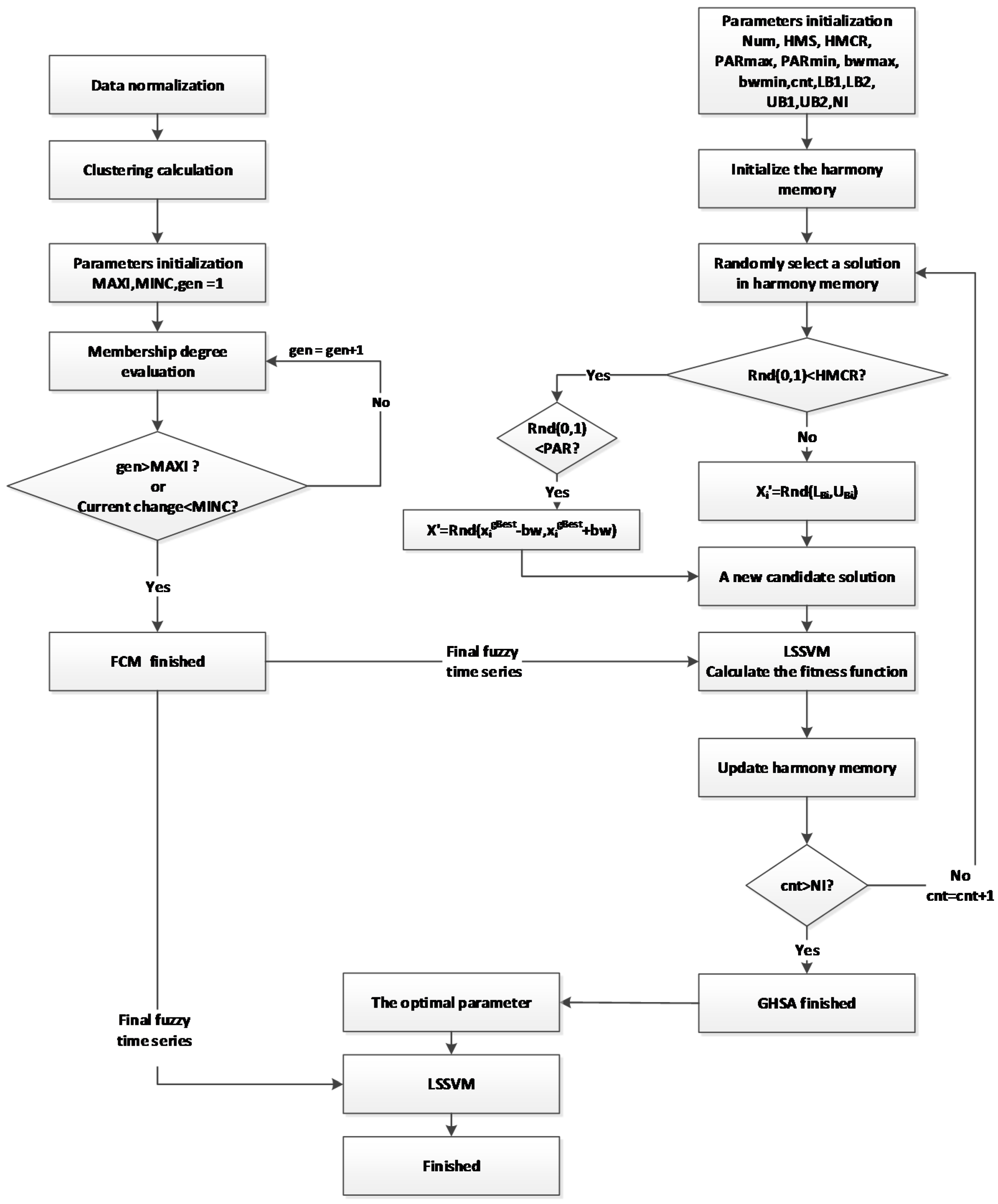
39]. The proposed GHSA procedure is illustrated as follows and the corresponding flowchart is shown in
Figure 1.
Step 1: Define the objective function and initialize parameters.
Firstly, is the objective function of the problem where x is a candidate solution consisting of N decision variables and . and are the lower and upper bounds for each variable. Besides, the parameters used in GHSA are also initialized in this step.
Step 2: Initialize the harmony memory.
The initialization process is done as:
Randomly generate a harmony memory in the size of from a uniform distribution in the range.
Calculate the fitness of each candidate solution in the harmony memory and sort the results in ascending order.
The harmony memory is generated by .
Step 3: Improvisation.
The purpose of this step is to generate a new harmony. The new harmony vector is generated based on the following rules:
Firstly, randomly generate
, in a uniform distribution of the range
.
If and , then . Palatino
If and , then , where is an arbitrary distance bandwidth (BW) and is dimension of the best candidate solution.
If , then .
Step 4: Update harmony memory.
If the fitness of the new harmony vector is better than that of the worst harmony, it will take the place of the worst harmony in the HM.
Step 5: Check the stopping criterion.
Terminate when the iteration is reached.
2.3. Fuzzy Time Series Generation
This paper proposes FCM model by using FCS algorithm with GA to process the raw data and to generate FTS. The flowchart is shown as
Figure 1. Firstly, the number of clustering
k is computed as the initial value. Secondly, the clustering center is obtained until the stop criteria of the algorithm are reached. Finally, the time series fuzzy membership is determined.
2.3.1. Fuzzy Time Series Model
A FTS is defined [
40,
41] as follows:
Definition 1:Let (t= 0, 1, 2,…), a subset of real number, be the universe of the discourse on which fuzzy membership of are defined. If F(t) is a collection of ,,…, then F(t) represents a FTS on Y(t).
Definition 2:If is caused by) only, the FTS relationship can be expressed as . Then let and, so the relationship between and which is referred to as a fuzzy logical relationship can be denoted by.
We present the general definitions of FTS as follows:
Suppose
U is divided into
n subsets, such as
. Then a fuzzy set
A in the universe of the discourse of
U can be expressed as Equation (6):
where
denotes the degree of membership of
in
A with the condition of
.
2.3.2. Fuzzy C-Means Clustering Algorithm
Fuzzy c-means (FCM) [
42] is a common clustering algorithm which could make one piece of data to cluster into multiple classes. Let
be the observation data set and
be the set of cluster centers. The results of fuzzy clustering can be expressed by membership function
where
and
is also limited by Equations (7) and (8).
Figure 1.
Global harmony search algorithm-fuzzy time series-least squares support vector machines (GHSA-FTS-LSSVM) algorithm flowchart.
Figure 1.
Global harmony search algorithm-fuzzy time series-least squares support vector machines (GHSA-FTS-LSSVM) algorithm flowchart.
The objective function of FCM can be express as Equation (9):
The cluster centers and the membership functions
are calculated by Equations (10) and (11):
where
is any real number named weight index,
represents the membership of
in the
cluster center and
refers to the Euclidean distance between the real value
and the fuzzy cluster center
.
3. Numerical Example
3.1. Data Set
The experiment employs electric load data of Guangdong Province Industrial Development Database to compare the forecasting performances among the proposed GHSA-FTS-LSSVM model, GHSA-LSSVM model, GA-LSSVM, PSO-LSSVM and GHSA-LSSVM. The detailed data used in this paper is shown in
Table 1. Among these data, the electric load data from January 2011 to December 2013 were used for model fitting and training, and the data from April to December 2014 were used to forecast.
Table 1.
Monthly electric load in Guangdong Province from January 2011 to November 2014 (unit: thousand million W/h).
Table 1.
Monthly electric load in Guangdong Province from January 2011 to November 2014 (unit: thousand million W/h).
| Date | Load | Date | Load | Date | Load |
|---|
| January 2011 | 284.1 | May 2012 | 351.6 | September 2013 | 372.3 |
| February 2011 | 263.2 | June 2012 | 353.1 | October 2013 | 375.6 |
| March 2011 | 339.8 | July 2012 | 386.5 | November 2013 | 386.4 |
| April 2011 | 325.7 | August 2012 | 376.1 | December 2013 | 410.9 |
| May 2011 | 336.2 | September 2012 | 338 | January 2014 | 384.5 |
| June 2011 | 341 | October 2012 | 343 | February 2014 | 322.1 |
| July 2011 | 371.7 | November 2012 | 356.1 | March 2014 | 389.2 |
| August 2011 | 366.4 | December 2012 | 362.4 | April 2014 | 373.3 |
| September 2011 | 329.8 | January 2013 | 331 | May 2014 | 387.6 |
| October 2011 | 326.9 | February 2013 | 278.1 | June 2014 | 393.4 |
| November 2011 | 331.4 | March 2013 | 368.3 | July 2014 | 429.8 |
| December 2011 | 362.3 | April 2013 | 357.2 | August 2014 | 416.7 |
| January 2012 | 341.5 | May 2013 | 368.1 | September 2014 | 379.9 |
| February 2012 | 328.3 | June 2013 | 373.3 | October 2014 | 385.3 |
| March 2012 | 358.7 | July 2013 | 419.4 | November 2014 | 398.2 |
| April 2012 | 335.2 | August 2013 | 426.6 | December 2014 | 374.8 |
The procedure of data preprocessing is illustrated as follows:
Step 1: Data normalization
Before FCM, we normalized the original data by Equation (12):
where
is the set of time series which contains
n observations,
and
refer to the minimum and maximum values of the data,
is the normalized set of time series.
Step 2: Clustering calculation.
The number of clustering
k is calculated by Equation (13) [
43]:
where ‘[]’ represents the rounded integer arithmetic. According to Equation (13),
.
Step 3: Parameters initialization
We determine the maximum iteration and the minimum change of membership . The performance of the algorithm depends on the initial cluster centers, so we need to specify a set of cluster centers at random.
Step 4: Update operator
If the objective function is better than the previous ones, the membership functions and cluster centers will be updated by Equations (10) and (11) after each iteration.
Step 5: Termination operator
In this paper, we use the iteration number and change of memberships as the termination operators. If the current iteration is larger than MAXI or the current change of membership is smaller than MINC, the FCM finish its work and we can get the cluster centers.
After FCM, we got a set of clustering centers (set = {0.6115, 0.4595, 3949, 0.6668, 0.9491, 0.0732, 0.7485, 0.5416}), and the final time series fuzzy membership we got is shown in
Table 2.
Table 2.
The final fuzzy time series (FTS) (partly).
Table 2.
The final fuzzy time series (FTS) (partly).
| Date | FTS |
|---|
| 11 January | 0.0104 | 0.0220 | 0.0338 | 0.0084 | 0.0036 | 0.9013 | 0.0063 | 0.0142 |
| 11 February | 0.0128 | 0.0227 | 0.0307 | 0.0108 | 0.0053 | 0.8928 | 0.0085 | 0.0163 |
| 11 March | 0.0000 | 1.0000 | 0.0000 | 0.0000 | 0.0000 | 0.0000 | 0.0000 | 0.0000 |
| 11 April | 0.0064 | 0.0506 | 0.9181 | 0.0042 | 0.0011 | 0.0039 | 0.0026 | 0.0130 |
| 11 May | 0.0115 | 0.7581 | 0.1842 | 0.0066 | 0.0013 | 0.0026 | 0.0036 | 0.0322 |
| 11 June | 0.0026 | 0.9743 | 0.0106 | 0.0014 | 0.0002 | 0.0004 | 0.0007 | 0.0099 |
| 11 July | 0.1255 | 0.0054 | 0.0030 | 0.8256 | 0.0022 | 0.0006 | 0.0210 | 0.0165 |
| 11 August | 0.9547 | 0.0024 | 0.0012 | 0.0272 | 0.0006 | 0.0002 | 0.0037 | 0.0101 |
| 11 September | 0.0005 | 0.0064 | 0.9911 | 0.0003 | 0.0001 | 0.0002 | 0.0002 | 0.0011 |
| 11 October | 0.0029 | 0.0256 | 0.9604 | 0.0019 | 0.0005 | 0.0016 | 0.0011 | 0.0060 |
| 11 November | 0.0046 | 0.0747 | 0.9032 | 0.0028 | 0.0006 | 0.0017 | 0.0016 | 0.0107 |
| 11 December | 0.8419 | 0.0127 | 0.0058 | 0.0449 | 0.0019 | 0.0009 | 0.0098 | 0.0821 |
3.2. Global Harmony Search Algorithm-Least Squares Support Vector Machines Model
3.2.1. Parameters Selection by Global Harmony Search Algorithm
Before the GHSA we need to determine parameters. The parameters include the number of variables, the range of each variable the harmony memory size (HMS), the harmony memory considering rate (HMCR), the value of BW, the pitch adjusting rate (PAR) and the number of iteration (NI).
In the experiments of GHSA, the larger harmony consideration rate (HMCR) is beneficial to the local convergence while the smaller HMCR can keep the diversity of the population. In this paper, we set the HMCR as 0.8. For the PAR, the smaller PAR can enhance the local search ability of algorithm while the larger PAR is easily to adjust search area around the harmony memory. In addition, the value of BW also has a certain impact on the searching results. For larger BW, it can avoid algorithm trapping into a local optimal and the smaller BW can search meticulously in the local area. In our experiment, we use a small PAR and a large BW in the early iterations of the algorithm, and with the increase of the NIs, BW is expected to be reduced while PAR ought to increase. Therefore, we adopt the following equations:
In swarm intelligence algorithms, the global optimization ability of algorithm will be ameliorated by increasing the population size increase. However, the search time will also increase and the convergence speed will slow down as the population size becomes larger. On the contrary, if the population size is small, the algorithm will more easily be trapped in a local optimum. The original data consists of 48 sets. Combined with the relevant research experiences and a lot of experiments, we divided the number of data by the number of parameters and the quotient we got is 24, which is set to be the HMS. After continuous optimization experiments, we determined 20 as the HMS in GHSA.
In the LS-SVM model, the regularization parameter,
, is a compromise to control the proportion of misclassification sample and the complexity of the model. It is used to adjust the empirical risk and confidence interval of data until the LS-SVM receiving excellent generalization performance. When the kernel parameter, σ, is approaching zero, the training sample can be correctly classified, however, it will suffer from over-fitting problem, and in the meanwhile, it will also reduce the generalization performance level of LS-SVM. Based on authors previous research experiences, the range of parameters
and σ we determined in this paper are [0, 10000], [0, 100]. The parameters we select in GHSA are shown in
Table 3.
Table 3.
Parameters selection in GHSA.
Table 3.
Parameters selection in GHSA.
| Parameter | Value | Comment |
|---|
| num | | Number of variables |
| | Range of each variable |
| | Range of each variable |
| | Harmony memory size |
| | HMS considering rate |
| , | Pitch adjusting rate |
| , | Bandwidth |
| | Number of iteration |
3.2.2. Fitness Function in Global Harmony Search Algorithm
Fitness function in GHSA is used to measure the fitness degree of generated harmony vector. Only if its fitness is better than that of the worst harmony in the harmony memory, it can replace the worst harmony. The fitness function is given Equation (16):
where
n refers to the number of test sample,
refers to the observation value and
to the predictive value in LSSVM.
Then we calculate the fitness function in GHSA by Equation (16). After finishing the GHSA, we have determined the optimal parameter and , then we establish LSSVM model to train historical data for forecasting the next electric load and get a set of output of LSSVM. At last, we denormalize the output of LSSVM.
3.2.3. Denormalization
After the GHSA we have determined the optimal parameter
and
, then we establish LSSVM model to train historical data for forecasting the next electric load. The outputs of LSSVM are normalized values, so we need to denormalize them to real values. Denormalization method is given by Equation (17):
where
max and
min refers to the maximum and minimum value of the original data.
3.2.4. Defuzzification Mechanism
As indicated by several experiments that there are some inherent errors between actual values and fuzzy values. Therefore, it's necessary to estimate this kind of fuzzy effects to provide higher accurate forecasting performance. In this paper, we proposed an approach to adjust the fuzzy effects, namely defuzzification mechanism, as shown in Equation (18):
where
for the twelve months in a year,
n is the total year number of data set,
refers to the number of year and
is the actual value and fuzzy value of the
year respectively. Thus, the final forecasting result can be expressed as Equation (19), and the defuzzification multipliers are shown in
Table 4.
Table 4.
Defuzzification multiplier of each month.
Table 4.
Defuzzification multiplier of each month.
| Month | Multiplier | Month | Multiplier |
|---|
| January | 1.00244 | July | 1.00612 |
| February | 0.98222 | August | 1.00567 |
| March | 0.99931 | September | 1.00069 |
| April | 0.99522 | October | 0.99932 |
| May | 0.99772 | November | 1.00937 |
| June | 1.00493 | December | 0.99996 |
3.3. Performance Evaluation
We compare these proposals in different respects. First the proposed GHSA efficiency is compared with other optimization algorithms like HSA, PSO and GA. These appropriate algorithms are utilized to optimize the parameter and .
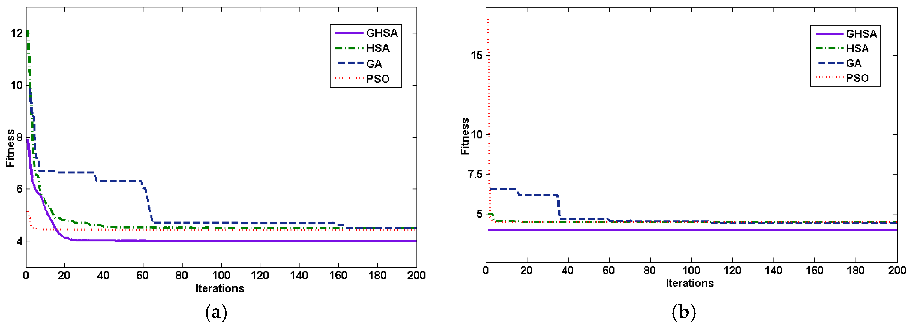
This experimental procedure is repeated 20 times for each optimization algorithm, and the performance comparison for different algorithms is represented in
Figure 2, and the comparison of average fitness curves is presented in
Table 5. We can see from
Figure 2 and
Table 5 that the values of the γ
−1 obtained by the four algorithms are close to 0.0001, that is, all the search algorithms can achieve similar optimization, but the values of parameter, σ, as optimized by the different algorithms are not the same and this directly affects the fitness. The convergence speed of PSO is the fastest, however, due to the algorithm complexity, its running time is long. The execution time of HSA is the shortest, but the fitness is the worst. The running time of GHSA is equivalent to HSA, and the fitness of GHSA is optimal among four algorithms. In second group, the forecasting accuracy of the proposed algorithm is compared with ARIMA, GA-LSSVM [
29], PSO-LSSVM [
30] and the first group models. We take the mean absolute percentage error (MAPE), mean absolute error (MAE) and root mean squared error (RMSE) to evaluate the accuracy of the proposed method. The MAPE are shown in Equations (20)–(22):
where
n refers to the number of sample,
is the observation value and
is the predictive value. According to the optimal value in
Table 5, forecasting results of GHSA-FTS-LSSVM, HSA-LSSVM, GA-LSSVM and PSO-LSSVM models as shown in
Table 6.
Figure 2.
Comparison of (a) average fitness curves; and (b) best fitness curves.
Figure 2.
Comparison of (a) average fitness curves; and (b) best fitness curves.
Table 5.
Performance comparison for different algorithms. Particle swarm optimization: PSO; harmony search algorithm: HAS; genetic algorithm: GA.
Table 5.
Performance comparison for different algorithms. Particle swarm optimization: PSO; harmony search algorithm: HAS; genetic algorithm: GA.
| Algorithm | Fitness | γ−1 | σ | Running Time/s |
|---|
| GHSA | 0.0397 | 0.00010 | 30.3977 | 9.2977 |
| HSA | 0.0489 | 0.00010 | 52.8422 | 8.2681 |
| GA | 0.0439 | 0.00010 | 52.8422 | 68.6248 |
| PSO | 0.0451 | 0.00011 | 22.3965 | 69.9352 |
Table 6.
Forecasting results of GHSA-FTS-LSSVM, GHSA-LSSVM, GA-LSSVM, PSO-LSSVM and autoregressive integrated moving average (ARIMA) models (unit: thousand million W/h).
Table 6.
Forecasting results of GHSA-FTS-LSSVM, GHSA-LSSVM, GA-LSSVM, PSO-LSSVM and autoregressive integrated moving average (ARIMA) models (unit: thousand million W/h).
| Time | Actual | GHSA-FTS-LSSVM | GHSA-LSSVM | GA-LSSVM [29] | PSO-LSSVM [30] | ARIMA |
|---|
| 15 January | 384.5 | 388.5989 | 387.094 | 387.066 | 393.205 | 399.142 |
| 15 February | 352.1 | 379.4326 | 372.661 | 372.65 | 373.62 | 381.038 |
| 15 March | 349.2 | 368.1298 | 355.006 | 355.01 | 352.864 | 359.864 |
| 15 April | 373.3 | 359.5839 | 353.429 | 353.434 | 351.189 | 377.003 |
| 15 May | 387.6 | 380.1802 | 366.55 | 366.545 | 366.026 | 362.173 |
| 15 June | 393.4 | 392.6603 | 374.353 | 374.341 | 375.799 | 361.905 |
| 15 July | 429.8 | 387.9569 | 377.522 | 377.506 | 379.962 | 399.488 |
| 15 August | 416.7 | 395.6517 | 397.452 | 397.409 | 408.614 | 432.612 |
| 15 September | 379.9 | 395.7048 | 390.271 | 390.239 | 397.814 | 423.027 |
| 15 October | 385.3 | 376.4279 | 370.15 | 370.142 | 370.449 | 404.338 |
| 15 November | 398.2 | 391.7981 | 373.098 | 373.086 | 374.179 | 390.129 |
| 15 December | 374.8 | 380.8968 | 380.146 | 380.127 | 383.494 | 385.307 |
| MAPE (%) | - | 3.709 | 4.579 | 4.579 | 4.654 | 5.219 |
| MAE | - | 14.358 | 18.035 | 18.035 | 18.215 | 20.153 |
| RMSE | - | 18.180 | 21.914 | 21.921 | 21.525 | 23.0717 |
The excellent performance of the GHSA-FTS-LSSVM method is due to following reasons: first of all, we use FCM to process the original data, making the accurate load value become a set of input variables with fuzzy feature. Thus, the defects of the original data can be overcome and the implicit information is dug up. Secondly, the proposed algorithm employed the GHSA to improve the searching efficiency. Finally, LSSVM reduces the time of equation solving and improves the accuracy and generalization ability of the model.


