1. Introduction
Electric energy can not be reserved, thus, electric load forecasting plays a vital role in the daily operational management of a power utility, such as energy transfer scheduling, unit commitment, load dispatch, and so on. With the emergence of load management strategies, it is highly desirable to develop accurate, fast, simple, robust and interpretable load forecasting models for these electric utilities to achieve the purposes of higher reliability and better management [
1].
In the past decades, researchers have proposed lots of methodologies to improve the load forecasting accuracy level. For example, Bianco
et al. [
2] proposed linear regression models for electricity consumption forecasting; Zhou
et al. [
3] applied a Grey prediction model for energy consumption; Afshar and Bigdeli [
4] presented an improved singular spectral analysis method to predict short-term load in the Iranian power market; and Kumar and Jain [
5] compared the forecasting performances among three Grey theory-based time series models to explore the consumption situation of conventional energy in India. Bianco
et al. [
6] indicate that their load model could be successfully used as an input of broader models than those of their previous paper [
2]. References [
7,
8,
9,
10] proposed several useful artificial neural networks models to conduct short-term load forecasting. The authors of [
11,
12,
13,
14] proposed hybrid models with evolutionary algorithms that demonstrated improved energy forecasting performances. These methods can achieve significant improvements in terms of forecasting accuracy, but without reasonable interpretability, particularly for ANN models. Artificial neural networks (ANNs), with mature nonlinear mapping capabilities and data processing characteristics, have achieved widely successful applications in load forecasting. Recently, expert systems with fuzzy rule-based linguistic means provided good interpretability while dealing with system modeling [
15]. Various approaches and models have been proposed in the last decades in many area such as climate factors (temperature and humidity), social activities (human social activities), seasonal factors (seasonal climate change and load growth), and so on. However, these models have strong dependency on an expert and lack expected forecasting accuracy. Therefore, combination models which are based on these popular methods and other techniques can satisfy the two desired requests: high accuracy level and interpretability.
With superiority in handling high dimension nonlinear data, support vector regression (SVR) has been successfully used to solve forecasting problems in many fields, such as financial time series (stocks index and exchange rate) forecasting, tourist arrival forecasting, atmospheric science forecasting, and so on [
16,
17,
18]. However, SVR methods have a significant disadvantage, in that while its three parameters are determined simultaneously during the nonlinear optimization process, the solution is easily trapped into a local optimum. In addition, it also lacks a statistically significant level of robustness. These two shortcomings are the focused topics in the SVR research field [
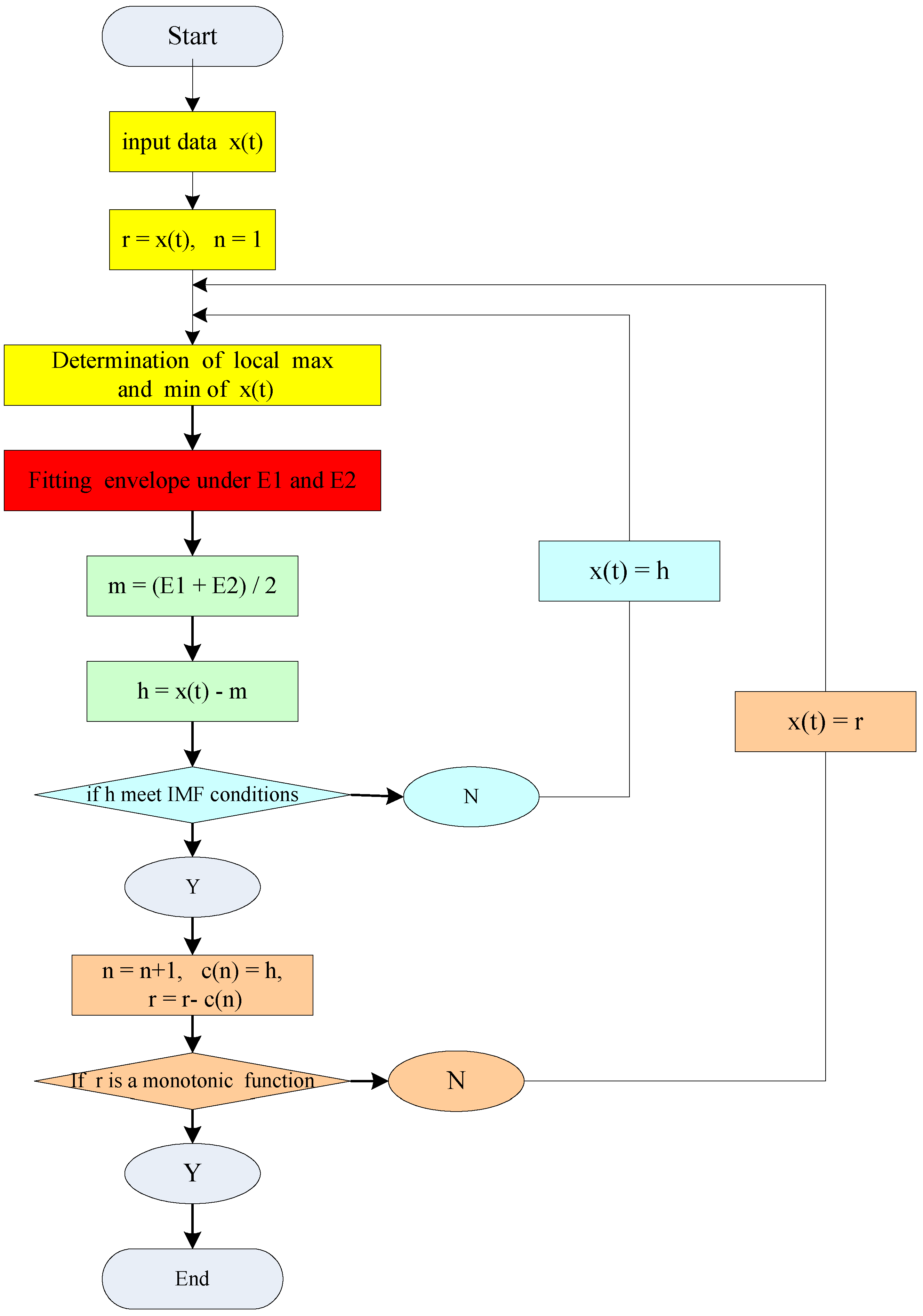
19]. On the other hand, the empirical mode decomposition (EMD) with auto regression (AR), a reliable clustering algorithm, has been successfully used in many fields [
20,
21,
22]. The EMD method is particularly powerful for extracting the components of the basic mode from nonlinear or non-stationary time series [
23],
i.e., the original complex time series can be transferred into a series of single and apparent components. However, this method cannot deal well with the signal decomposition effects while the gradient of the time series is fluctuating. Based on the empirical decomposition mode, reference [
24] proposes the differential empirical mode decomposition (DEMD) to improve the fluctuating changes problem of the original EMD method. The derived signal is obtained by several derivations of the original signal, and the fluctuating gradient is thus eliminated, so that the signal can satisfy the conditions of EMD. The new signal is then integrated into EMD to obtain each intrinsic mode function (IMF) order and the residual amount of the original signal. The differential EMD method is employed to decompose the electric load into several detailed parts with higher frequency IMF and an approximate part with lower frequencies. This can effectively reduce the unnecessary interactions among singular values and can improve the performance when a single kernel function is used in forecasting. Therefore, it is beneficial to apply a suitable kernel function to conduct time series forecasting [
25]. Since 1995, many attempts have been made to improve the performance of the PSO [
26,
27,
28,
29,
30,
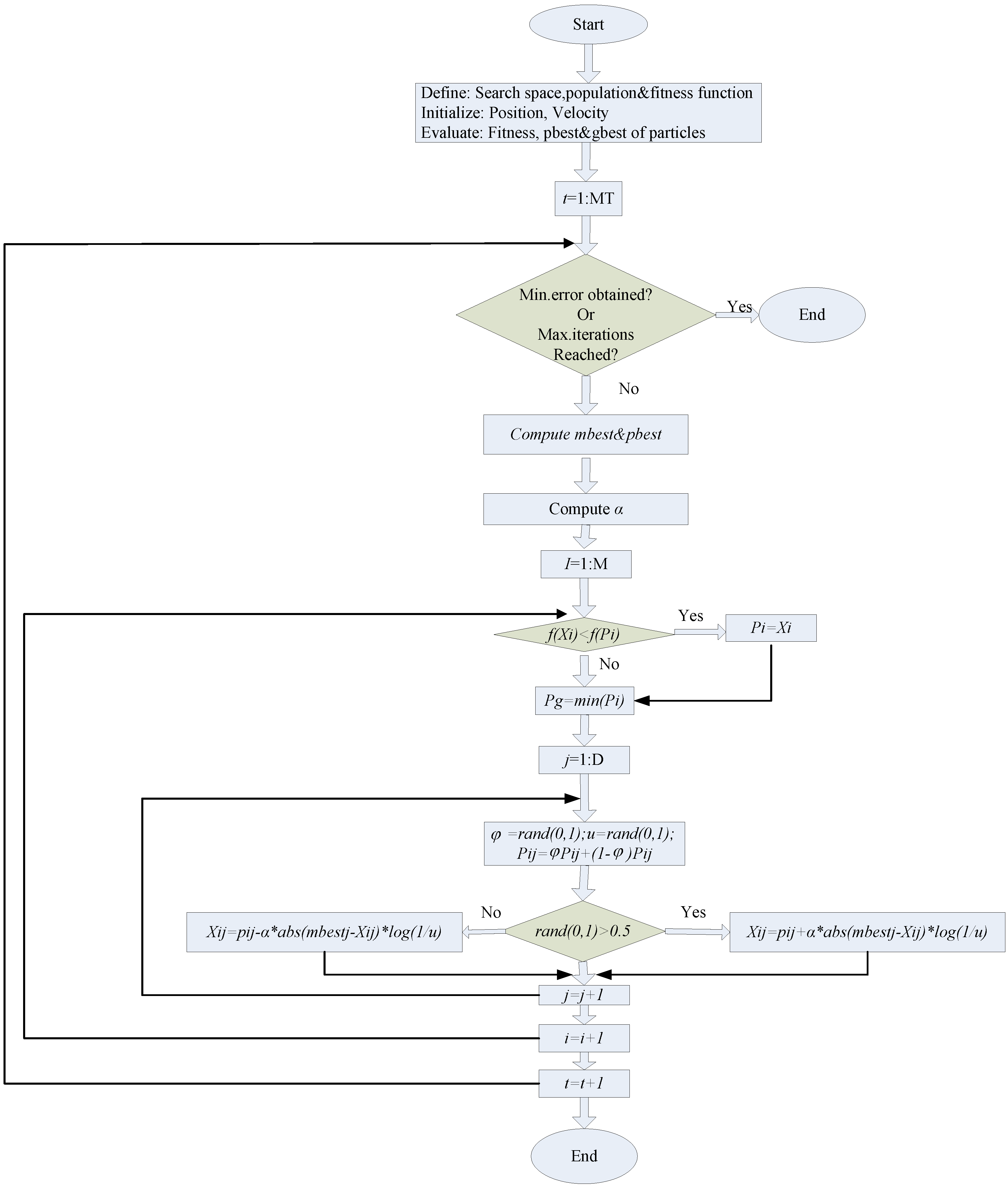
31]. Sun
et al. [
32,
33] introduced quantum theory into PSO and proposed a quantum-behaved PSO (QPSO) algorithm, which is a global search algorithm to theoretically guarantee finding good optimal solutions in the search space. Compared with PSO, the iterative equation of QPSO needs no velocity vectors for particles, has fewer parameters to adjust, and can be implemented more easily. The results of experiments on widely used benchmark functions indicate that the QPSO is a promising algorithm [
32,
33] that exhibits better performance than the standard PSO.
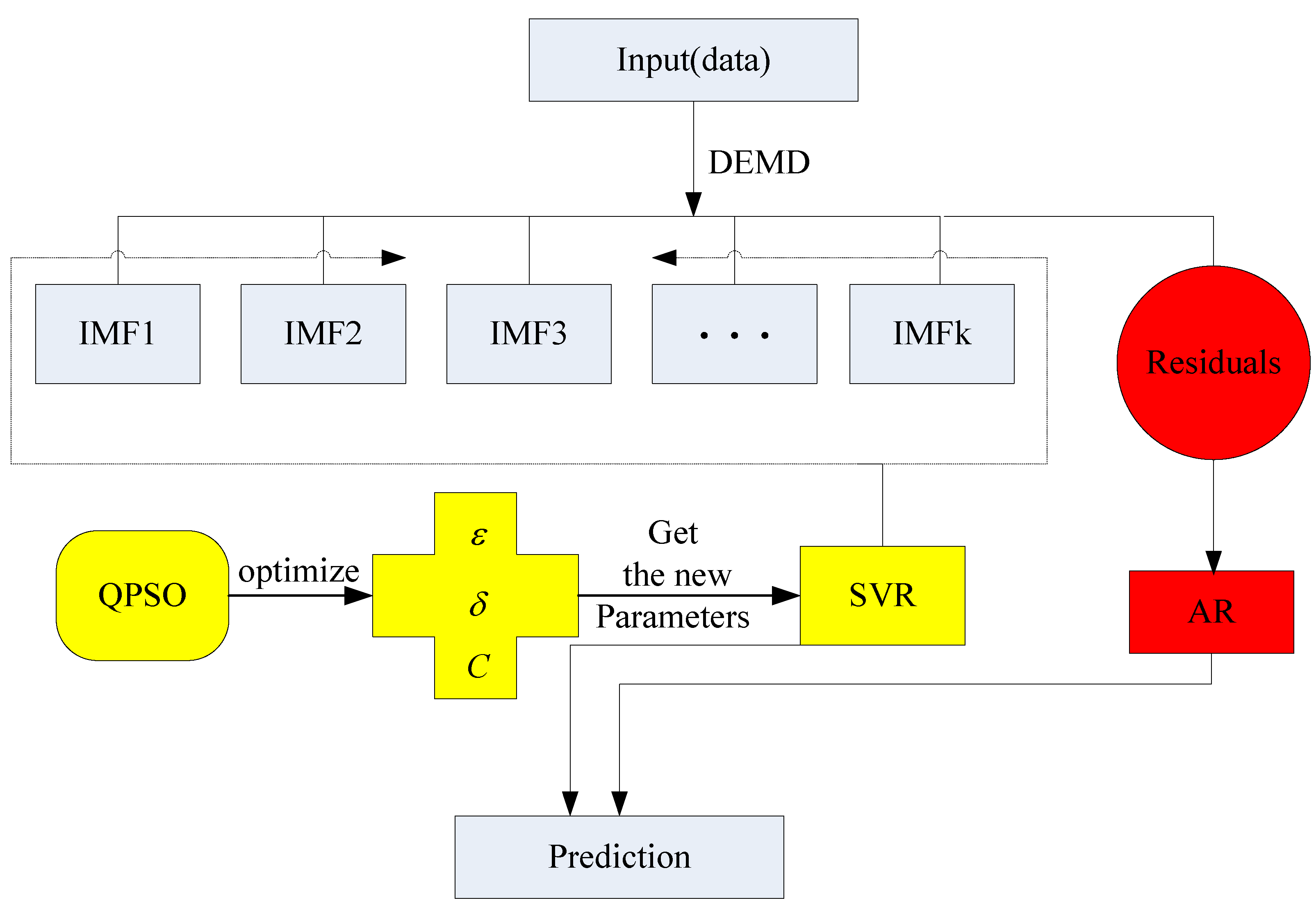
In this paper, we present a new hybrid model to achieve satisfactory forecasting accuracy. The principal idea is hybridizing DEMD with QPSO, SVR and AR, namely the DEMD-QPSO-SVR-AR model, to achieve better forecasting performance. The outline of the proposed DEMD-QPSO-SVR-AR model is as follows: (1) the raw data can be divided into two parts by DEMD technology, one is the higher frequency item, the other is the residuals; (2) the higher frequency item has less redundant information than the raw data and trend information, because that information is gone to the residuals, then, QPSO is applied to optimize the parameters of SVR (i.e., the so-called QPSO-SVR model), so the QPSO-SVR model is used to forecast the higher frequency, the accuracy is higher than the original SVR model, particularly around the peak value; (3) fortunately, the residuals is monotonous and stationary, so the AR model is appropriate for forecasting the residuals; (4) the forecasting results are obtained from Steps (2) and (3). The proposed DEMD-QPSO-SVR-AR model has the capability of smoothing and reducing the noise (inherited from DEMD), the capability of filtering dataset and improving forecasting performance (inherited from SVR), and the capability of effectively forecasting the future tendencies (inherited from AR). The forecast outputs obtained by using the proposed hybrid method are described in the following sections.
To show the applicability and superiority of the proposed model, half-hourly electric load data (48 data points per day) from New South Wales (Australia) with two kind of sizes are used to compare the forecasting performances among the proposed model and other four alternative models, namely the PSO-BP model (BP neural network trained by the PSO algorithm), SVR model, PSO-SVR model (optimizing SVR parameters by the PSO algorithm), and the AFCM model (adaptive fuzzy combination model based on a self-organizing mapping and SVR). Secondly, another hourly electric load dataset (24 data points per day) from the New York Independent System Operator (NYISO, USA), also, with two kinds of sizes are used to further compare the forecasting performances of the proposed model with other three alternative models, namely the ARIMA model, BPNN model (artificial neural network trained by a back-propagation algorithm), and GA-ANN model (artificial neural network trained by a genetic algorithm). The experimental results indicate that this proposed DEMD-QPSO-SVR-AR model has the following advantages: (1) it simultaneously satisfies the need for high levels of accuracy and interpretability; (2) the proposed model can tolerate more redundant information than the SVR model, thus, it has more powerful generalization ability.
The rest of this paper is organized as follows: in
Section 2, the DEMD-QPSO-SVR-AR forecasting model is introduced and the detailed illustrations of the model are also provided. In
Section 3, the data description and the research design are illustrated. The numerical results and comparisons are shown in
Section 4. The conclusions of this paper and the future research focuses are given in
Section 5.
3. Numerical Examples
To illustrate the superiority of the proposed model, we use two datasets from different electricity markets, that is, the New South Wales (NSW) market in Australia (denoted as Case 1) and the New York Independent System Operator (NYISO) in the USA (Case 2). In addition, for each case, we all use two sample sizes, called small sample and large sample, respectively.
3.1. The Experimental Results of Case 1
For Case 1, firstly, electric load data obtained from 2 to 7 May 2007 is used as the training data set in the modeling process, and the testing data set is from 8 May 2007. The electric load data used are all based on a half-hourly basis (i.e., 48 data points per day). The dataset containing only 7 days is called the small size sample in this paper.
Secondly, for large training sets, it should avoid overtraining during the SVR modeling process. Therefore, the second data size has 23 days (1104 data points from 2 to 24 May 2007) by employing all of the training samples as training set, i.e., from 2 to 17 May 2007, and the testing data set is from 18 to 24 May 2007. This example is called the large sample size data in this paper.
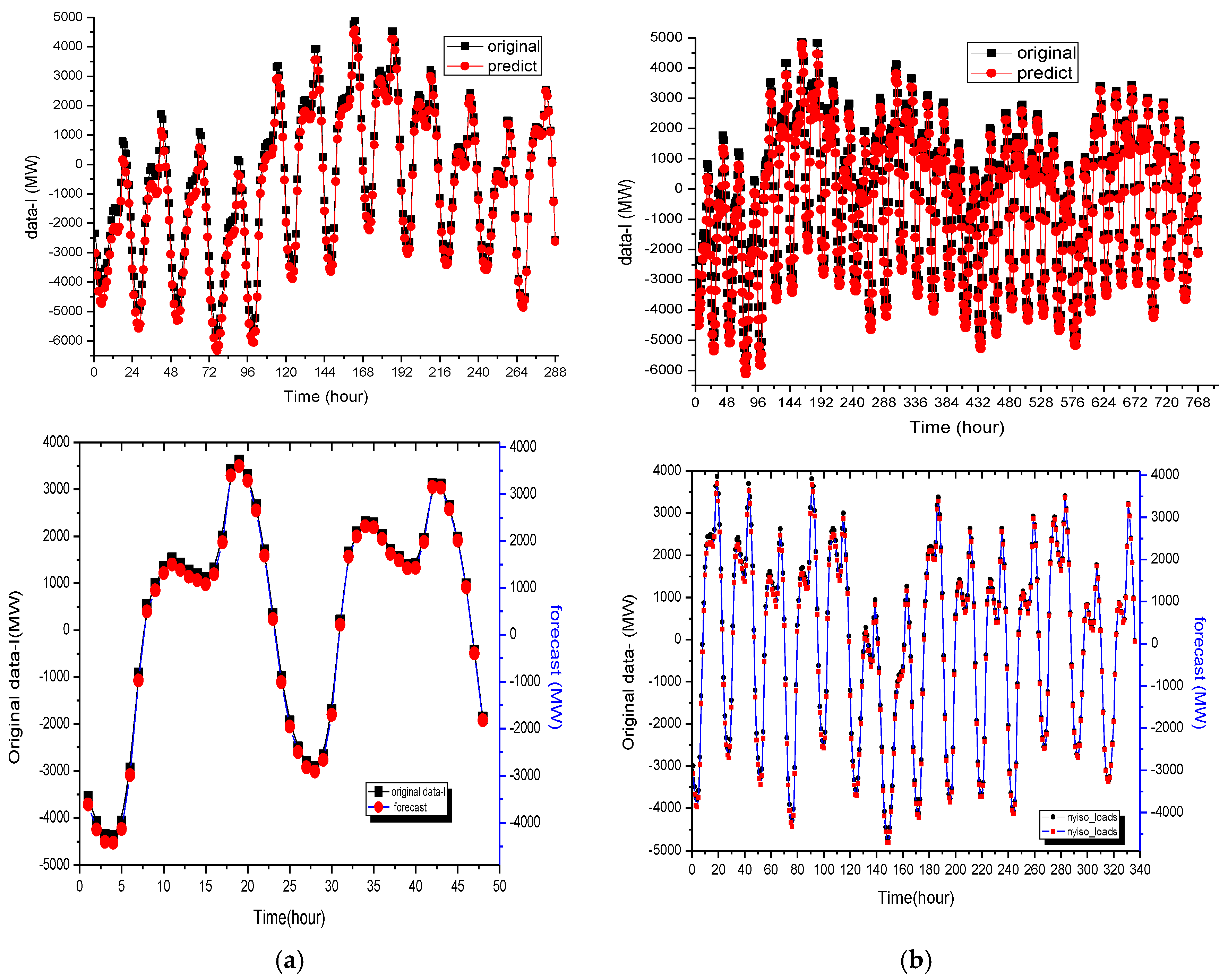
(i) Results after DEMD in Case 1
As mentioned in the authors’ previous paper [
25], the results of the decomposition process by DEMD, can be divided into the higher frequency item (Data-I) and the residuals term (Data-II). The trend of the higher frequency item is the same as that of the original data, and the structure is more regular and stable. Thus, Data-I and Data-II both have good regression effects by the QPSO-SVR and AR, respectively.
(ii) Forecasting Using QPSO-SVR for Data-I (The Higher Frequency Item in Case 1)
After employing DEMD to reduce the non-stationarity of the data set in Case 1, QPSO with SVR can be successfully applied to reduce the performance volatility of SVR with different parameters, to perform the parameter determination in SVR modeling process.
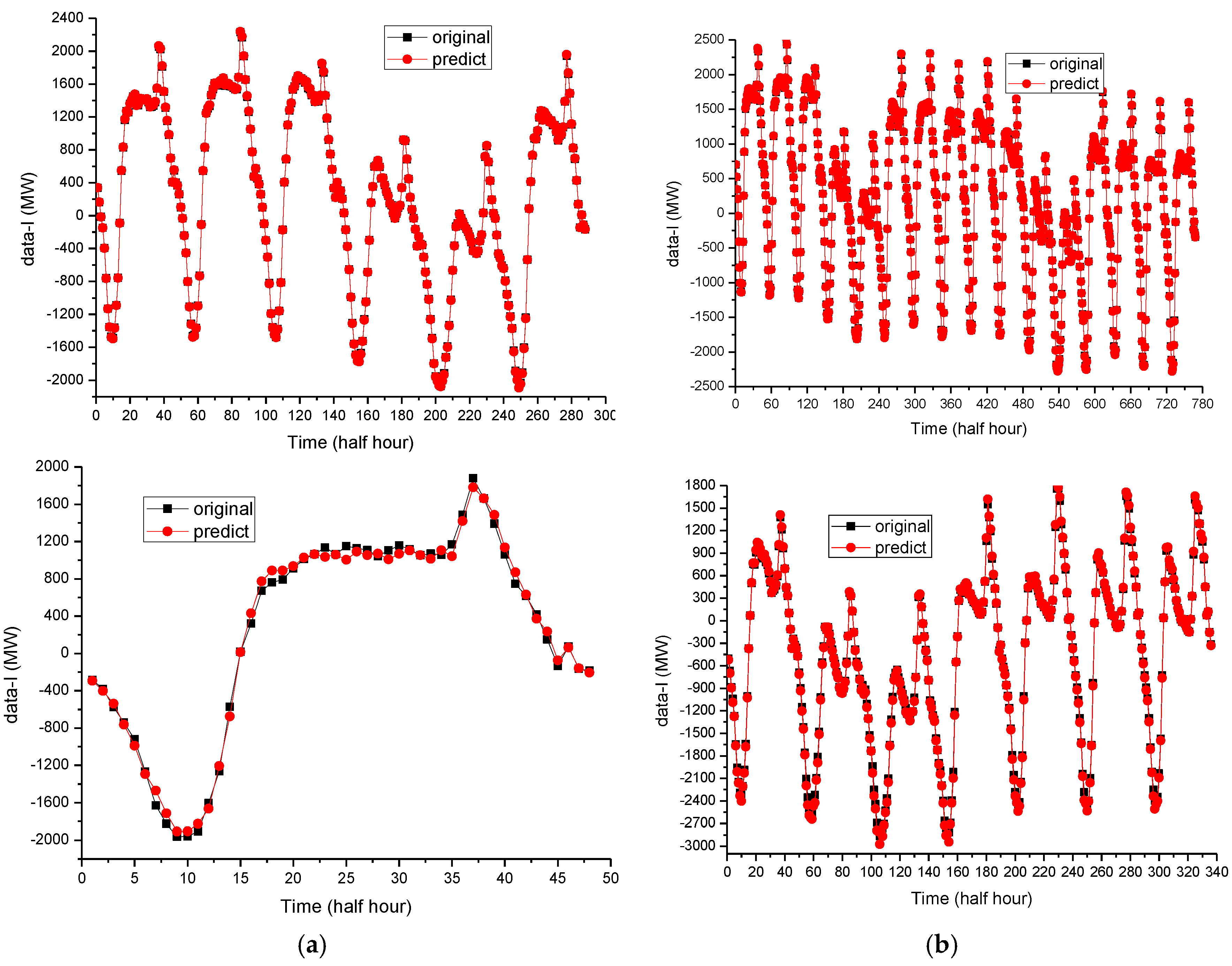
The higher frequency item is simultaneously employed for QPSO-SVR modeling, and the better performances of the training and testing (forecasting) sets are shown in
Figure 4a,b, respectively. This implies that the decomposition and optimization by QPSO is helpful to improve the forecasting accuracy. The parameters of a QPSO-SVR model for Data-I are shown in
Table 1 and
Table 2, in which the forecasting error for the higher frequency decomposed by the DEMD and QPSO-SVR has been reduced.
Where N is number of particles, Cmin is the minimum of C, Cmax is the maximum of C, σmin is the minimum of σ, σmax is the maximum of σ, itmax is maximum iteration number.
(iii) Forecasting Using AR for Data-II (The Residuals in Case 1)
As mentioned in the authors’ previous paper [
25], the residuals are linear locally and stable, so use of the AR technique to predict Data-II is feasible. Based on the geometric decay of the correlation analysis for Data-II (the residuals), it can be denoted as the AR(4) model. The associated parameters of the AR(4) model for Data-II are indicated in
Table 3. The errors almost approach the level of 10
−5 both for the small or large amounts of data,
i.e., the forecasting error for Data-II by DEMD has been significantly reduced. This shows the superiority of the AR model.
3.2. The Experimental Results of Case 2
For Case 2, electric load data obtained from 1 to 12 January 2015 is used as the training data set in the modeling process, and the testing data set is from 13 to 14 January 2015. These employed electric load data are all based on an hour basis (i.e., 24 data points per day). The dataset contains only 14 days so it is also called the small sample in this paper.
Secondly, for large training sets, the second dataset size is 46 days (1104 data points from 1 January to 15 February 2015) by employing all of the training samples as training set, i.e., from 1 January to 1 February 2015, and the testing dataset is from 2 to 15 February 2015. This example is also called the large size sample data in this paper.
(i) Results after DEMD in Case 2
As mentioned in the authors’ previous paper [
25], similarly, the data results of the decomposition process by DEMD can be divided into the higher frequency item (Data-I) and the residuals term (Data-II). The trend of the higher frequency item is also the same as that of the original data, and the structure is also regular and stable. Thus, Data-I and Data-II both have good regression effects by the QPSO-SVR and AR, respectively.
(ii) Forecasting Using QPSO-SVR for Data-I (The Higher Frequency Item in Case 2)
After employing DEMD to reduce the non-stationarity of the data set in Case 2, to further resolve these complex nonlinear, chaotic problems for both small sample and large sample data, the QPSO with SVR can be successfully applied to reduce the performance volatility of SVR with different parameters to perform the parameter determination in the SVR modeling process, to improve the forecasting accuracy. The higher frequency item is simultaneously employed for QPSO-SVR modeling, and the better performances of the training and testing (forecasting) sets are shown in
Figure 5a,b, respectively. This implies that the decomposition and optimization by QPSO is helpful to improve the forecasting accuracy. The parameters of a QPSO-SVR model for Data-I are shown in
Table 1 and
Table 4, in which the forecasting error for the higher frequency decomposed by the DEMD and QPSO-SVR has been reduced.
(iii) Forecasting Using AR for Data-II (The Residuals in Case 2)
As mentioned in the authors’ previous paper [
25], the residuals are linear locally and stable, so the AR technique is feasible to predict Data-II. Based on the geometric decay of the correlation analysis for Data-II (the residuals), that can also be denoted as the AR(4) model, the associated parameters of the AR(4) model for Data-II are indicated in
Table 5. The errors almost approach a level of 10
−5 both for the small or large amount of data,
i.e., the forecasting error for Data-II by DEMD has significantly reduced. This shows the superiority of the AR model.
Where xn is the n-th electric load residual, xn-1 is the (n − 1)th electric load residual similarly, etc.
4. Results and Analysis
This section illustrates the performance of the proposed DEMD-QPSO-SVR-AR model in terms of forecasting accuracy and interpretability. Taking into account the superiority of an SVR model for small sample size and superiority comparisons, a real case analysis with small sample size is used in the first case. The next case with 1104 data points is devoted to illustrate the relationships between two sample sizes (large size and small size) and accurate levels in forecasting.
4.1. Setting Parameters for the Proposed Forecasting Models
As indicated by Taylor [
46], and according to the same conditions of the comparison with Che
et al. [
47], the settings of several parameters in the proposed forecasting models are illustrated as follows. For the PSO-BP model, 90% of the collected samples is used to train the model, and the rest (10%) is employed to test the performance. In the PSO-BP model, these used parameters are set as follows: (i) for the BP neural network, the input layer dimension (
indim) is set as 2; the dimension of the hidden layer (
hiddennum) is set as 3; the dimension of the output layer (
outdim) is set as 1; (ii) for the PSO algorithm, the maximum iteration number (
itmax) is set as 300; the number of the searching particles,
N, is set as 40; the length of each particle,
D, is set as 3; weight
c1 and
c2 are set as 2.
The PSO-SVR model not only has its embedded constraints and limitations from the original SVR model, but also has huge iteration steps as a result of the requirements of the PSO algorithm. Therefore, it would be time consuming to train the PSO-SVR model while the total training set is used. For this consideration, the total training set is divided into two sub-sets, namely training subset and evaluation subset. In the PSO algorithm, the parameters used are set as follows: for the small sample, the maximum iteration number (itmax) is set as 50; the number of the searching particles, N, is set as 20; the length of each particle, D, is set as 3; weight c1 and c2 are set as 2; for the large sample, the maximum iteration number (itmax) is set as 20; the number of the searching particles, N, is set as 5; the length of each particle, D, is also set as 3; weight c1 and c2 are also set as 2.
Regarding Case 2, to be based on the same comparison conditions used in Fan
et al. [
25], the newest electric load data from NYISO is also employed for modeling, five alternative forecasting models (including the ARIMA, BPNN, GA-ANN, EMD-SVR-AR, and DEMD-SVR-AR models) are used for comparison with the proposed model. Some parameter settings of the employed forecasting models are set the same as in [
25], and are briefly as follows: for the BPNN model, the node numbers of its structure are different for small sample size and large sample size; for the former one, the input layer dimension is 240, the hidden layer dimension is 12, and the output layer dimension is 48; and these values are 480, 12, 336, respectively, for the latter one. The parameters of GA-ANN model used in this case are as follows: generation number is set as 5, population size is set as 100, bit numbers are set as 50, mutation rate is set as 0.8, crossover rate is 0.05.
4.2. Evaluation Indices for Forecasting Performances
For evaluating the forecasting performances, three famous forecasting accurate level indices, RMSE (root mean square error), MAE (mean absolute error), and MAPE (mean absolute percentage error), as shown in Equations (24) to (26), are employed:
where
Pi and
Ai are the
i-th forecasting and actual values, respectively, and
n is the total number of forecasts.
In addition, to verify the suitability of model selection, Akaike’s Information Criterion (AIC), an index of measurement for the relative quality of models for a given set of data, and Bayesian Information Criterion (BIC), also known as the Schwartz criterion, which is a criterion for model selection among a finite set of models (the model with the lowest BIC is preferred), are both taken into account to enhance the robustness of the verification. These two indices are defined as Equations (27) and (28), respectively:
where
SSE is the sum of squares for errors,
q is the number of estimated parameters:
where
q is the number of estimated parameters and
n is the sample size.
4.3. Empirical Results and Analysis
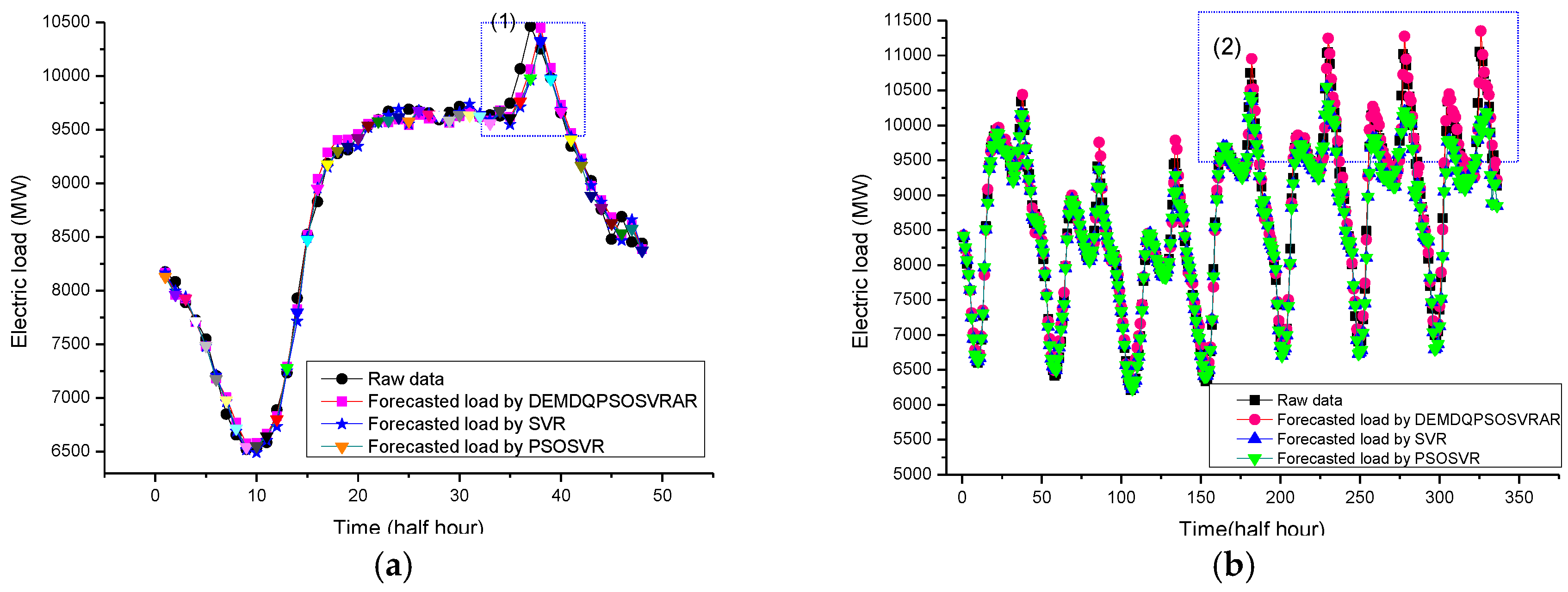
For the first experiment in Case 1, the forecasting results (the electric load on 8 May 2007) of the original SVR model, the PSO-SVR model and the proposed DEMD-QPSO-SVR-AR model are shown in
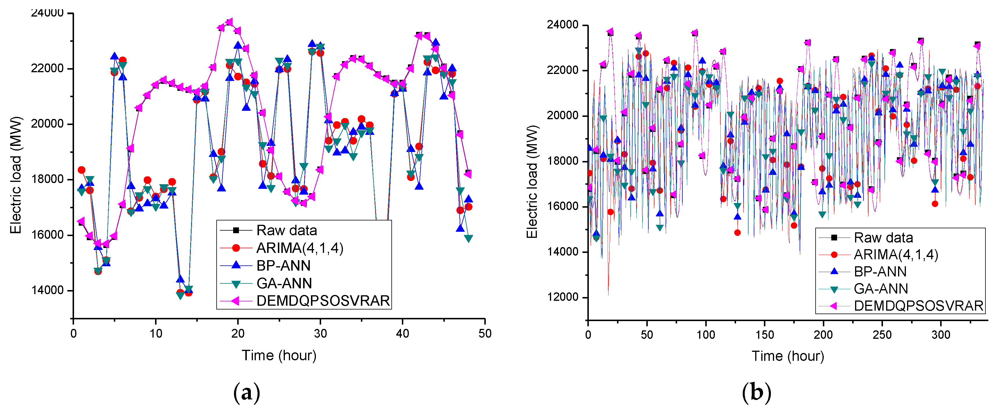
Figure 6a. For Case 2, the forecasting results of the ARIMA model, the BPNN model, the GA-ANN model and the proposed DEMD-QPSO-SVR-AR model are shown in
Figure 7a. Based on these two figures, the forecasting curve of the proposed DEMD-QPSO-SVR-AR model seems to achieve a better fit than other alternative models for the two cases in this experiment.
The second experiments in Cases 1 and 2 show the large sample size data. The peak load values of the testing set are bigger than those of the training set. The detailed forecasting results in this experiment are illustrated in
Figure 6b and
Figure 7b. It also shows that the results obtained from the proposed DEMD-QPSO-SVR-AR model seem to have smaller forecasting errors than other alternative models.
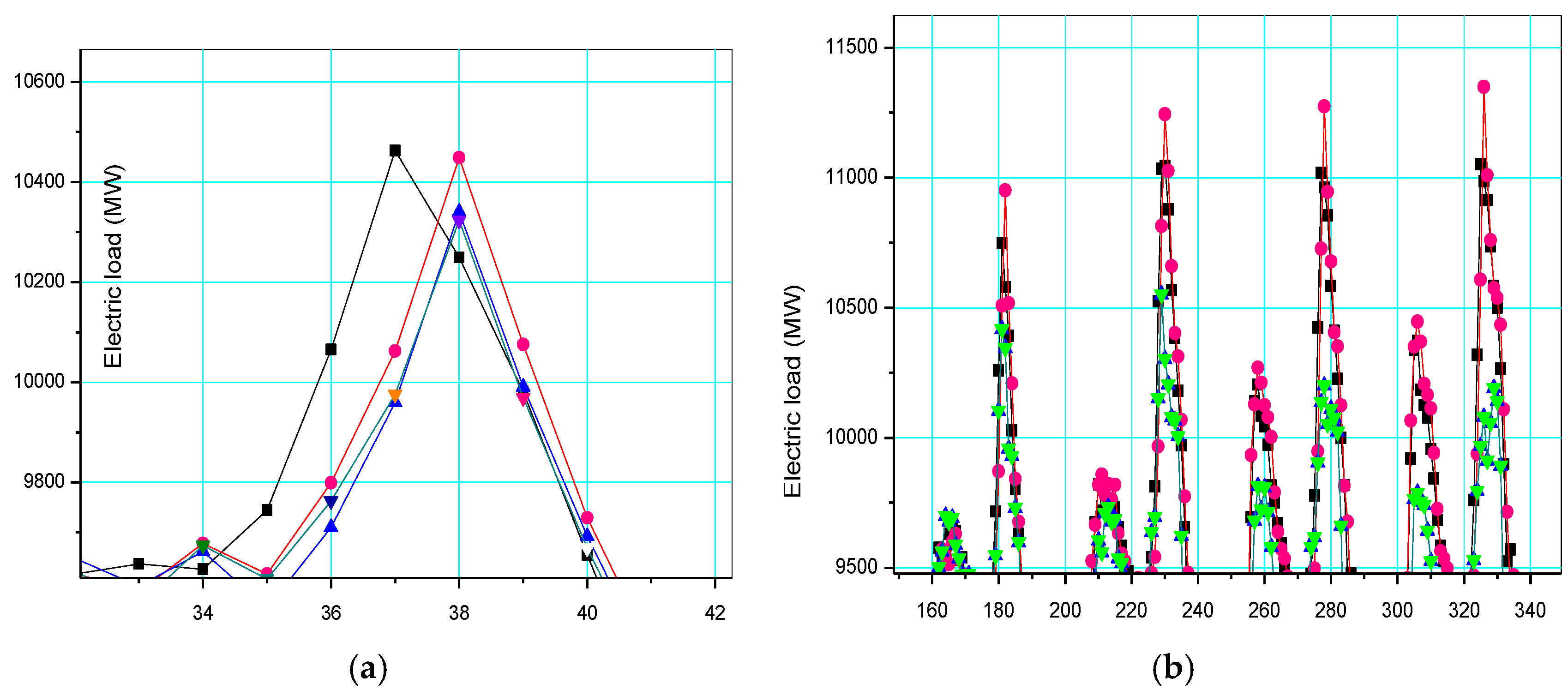
Notice that for any particular sharp points in
Figure 6 and
Figure 7, after extracting the direction feature of the trend by DEMD technology, these sharp points fixed in their positions represent the higher frequency characteristics of the remaining term, therefore, quantizing the particles in PSO the algorithm is very effective for dealing with this kind of fixed point characteristics. In other words, the DEMD-QPSO-SVR-AR model has better generalization ability than other alternative comparison models in both cases. Particularly in Case 1, for example, the local details for sharp points in
Figure 6a,b are enlarged and are shown in
Figure 8a,b, respectively. It is clear that the forecasting curve of the proposed DEMD-QPSO-SVR-AR model (red solid dots and red curve) fits more precisely than other alternative models,
i.e., it is superior for capturing the data change trends, including any fluctuation tendency.
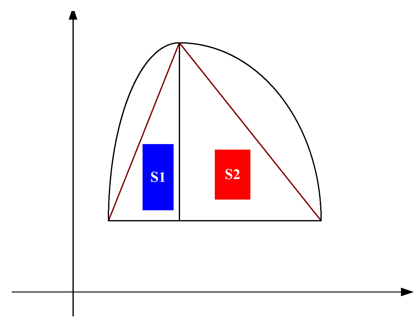
To better explain the superiority, the shape factor (
SF), defined as Equation (29) and shown in
Figure 9, is employed to illustrate the fitting effectiveness of the method, the
SF value of the model closer to the one of the raw data, the fitness of the model is better than others. The results are shown in
Table 6. It indicates that the data of
SF from DEMD-QPSO-SVR-AR model is closer to the raw data than other models:
The forecasting results in Cases 1 and 2 are summarized in
Table 7 and
Table 8, respectively. The proposed DEMD-QPSO-SVR-AR model is compared with alternative models. It is indicated that our hybrid model outperforms all other alternatives in terms of all the evaluation criteria. One of the general observations is that the proposed model tends to fit closer to the actual value with a smaller forecasting error. This is ascribed to the fact that a well combined DEMD and QPSO can effectively capture the exact shape characteristics, which are difficult to illustrate by many other methods while data often has intertwined effects among the chaos, noise, and other unstable factors. Therefore, the unstable impact is well solved by DEMD, especially for those border points, and then, QPSO can accurately illustrate the chaotic rules,
i.e., achieve more satisfactory parameter solutions for an SVR model.
In view of the model effectiveness and efficiency on the whole, we can conclude that the proposed model is quite competitive against other compared models, such as the ARIMA, BPNN, GA-ANN, PSO-BP, SVR, PSO-SVR, and AFCM models. In other words, the hybrid model leads to better accuracy and statistical interpretation.
In particular, as shown in
Figure 8, our method shows higher accuracy and good flexibility in peak or inflection points, because the little redundant information could be used by statistical learning or regression models, and the level of optimization would increase. This also ensures that it could achieve more significant forecasting results due to the closer
SF values to the raw data set. For closer insight, this can be viewed as the fact that the shape factor reflects how the electric load demand mechanism ia affected by multiple factors,
i.e., the shape factor reflects the change tendency in terms of ups or downs, thus, closer SF value to the raw data set can capture more precise trend changes than others, and this method no doubt can reveal the regularities for any point status.
Several findings deserved to be noted. Firstly, based on the forecasting performance comparisons among these models, the proposed model outperforms other alternative models. Secondly, the proposed model has better generalization ability for different input patterns as shown in the second experiment. Thirdly, from the comparison between the different sample sizes of these two experiments, we conclude that the hybrid model can tolerate more redundant information and construct the model for the larger sample size data set. Fourthly, based on the calculation and comparison of
SF in
Table 6, the proposed model also receives closer
SF values to the raw data than other alternative models. Finally, since the proposed model generates good results with good accuracy and interpretability, it is robust and effective, as shown in
Table 7 and
Table 8, comparing the other models, namely the original SVR, PSO-SVR, PSO-BP and AFCM models. Overall, the proposed model provides a very powerful tool that is easy to implement for electric load forecasting.
Eventually, the most important issue is to verify the significance of the accuracy improvement of the proposed model. The forecasting accuracy comparisons in both cases among original SVR, PSO-SVR, PSO-BP, AFCM, ARIMA, BPNN, and GA-ANN models are conducted by a statistical test, namely a Wilcoxon signed-rank test, at the 0.025 and 0.05 significant levels in one-tail-tests. The Wilcoxon signed-rank test is a non-parametric statistical hypothesis test used when comparing two related samples, matched samples, or repeated measurements on a single sample to assess whether their population mean ranks differ (
i.e., it is a paired difference test). It can be used as an alternative to the paired Student’s t-test, t-test for matched pairs, or the
t-test for dependent samples when the population cannot be assumed to be normally distributed [
48]. The test results are shown in
Table 9 and
Table 10. Clearly, the outstanding forecasting results achieved by the proposed model is only significantly superior to other alternative models at a significance level of 0.05. This also implies that there are still lots of improvement efforts that can be made for hybrid quantum-behavior evolutionary SVR-based models.
5. Conclusions
This paper presents an SVR model hybridized with the differential empirical mode decomposition (DEMD) method and quantum particle swarm optimization algorithm (QPSO) for electric load forecasting. The experimental results indicate that the proposed model is significantly superior to the original SVR, PSO-SVR, PSO-BP, AFCM, ARIMA, BPNN, and GA-ANN models. To improve the forecasting performance (accuracy level), quantum theory is hybridized with PSO (namely the QPSO) into an SVR model to determine its suitable parameter values. Furthermore, the DEMD is employed to simultaneously consider the accuracy and comprehensibility of the forecast results. Eventually, a hybrid model (namely DEMD-QPSO-SVR-AR model) has been proposed and its electric load forecasting superiority has also been compared with other alternative models. It is also demonstrated that a well combined DEMD and QPSO can effectively capture the exact shape characteristics, which are difficult to illustrate by many other methods while data often has intertwined effects among the chaos, noise, and other unstable factors. Hence, the instability impact can be well solved by DEMD, especially for those border points, and then, QPSO can accurately illustrate the chaotic rules, thus achieving more satisfactory parameter solutions than an SVR model.


