A Carbon Price Forecasting Model Based on Variational Mode Decomposition and Spiking Neural Networks

Abstract

Accurate forecasting of carbon price is important and fundamental for anticipating the changing trends of the energy market, and, thus, to provide a valid reference for establishing power industry policy. However, carbon price forecasting is complicated owing to the nonlinear and non-stationary characteristics of carbon prices. In this paper, a combined forecasting model based on variational mode decomposition (VMD) and spiking neural networks (SNNs) is proposed. An original carbon price series is firstly decomposed into a series of relatively stable components through VMD to simplify the interference and coupling across characteristic information of different scales in the data. Then, a SNN forecasting model is built for each component, and the partial autocorrelation function (PACF) is used to determine the input variables for each SNN model. The final forecasting result for the original carbon price can be obtained by aggregating the forecasting results of all the components. Actual InterContinental Exchange (ICE) carbon price data is used for simulation, and comprehensive evaluation criteria are proposed for quantitative error evaluation. Simulation results and analysis suggest that the proposed VMD-SNN forecasting model outperforms conventional models in terms of forecasting accuracy and reliability.

1. Introduction

Global warming induced by fossil fuel consumption has become a formidable challenge faced by all countries, which has spurred the development of socialized economies. Correspondingly, a worldwide consensus has emerged to foster a clean, high efficiency and low-carbon energy system. The Kyoto Protocol agreement officially came into force in 2005, marking the beginning of greenhouse gas reduction by leveraging a market mechanism [1]. Henceforth, the carbon trading market has expanded worldwide. As one of the primary sources of carbon emissions, the power industry has a dramatic potential for carbon emissions reduction and obvious scope for optimization. In the past two decades, numerous studies have been conducted regarding power system planning and dispatching under market circumstances that take into account carbon trading and, in particular, future carbon prices [2,3,4]. Therefore, the development of a reliable carbon price forecasting and analysis approach is the key to anticipating the changing trends of the energy market, and, thus, to provide a valid reference for establishing power industry policy.

Recently, carbon price forecasting has attracted considerable worldwide attention. Generally speaking, existing models and methods that have been adopted can be mainly divided into two categories: single models [5,6,7] and combined models [8,9,10]. Single model forecasting mainly uses generalized autoregressive conditional heteroskedasticity (GARCH)-type models or artificial neural networks (ANNs) to analyze and simulate a carbon price time series, and then employs the developed model to forecast the carbon price. For example, various types of GARCH models, including GARCH, EGARCH and TGARCH, have been proposed [5] to forecast and analyze the volatility of European Union allowance (EUA) spot and futures. The forecasting effect of single variable and multivariable GARCH models in the energy market has also been evaluated [6]. These types of GARCH models are statistical models that are not able to capture the nonlinear characteristics of the carbon price time series effectively, which affects the forecasting accuracy. Compared with statistical models, ANNs possess strong self-learning and adaptive capabilities, and can perform complex nonlinear mapping [7]. Nevertheless, ANNs face substantial challenges in dealing with large historical data sets, which also limits forecasting accuracy. Spiking neural networks (SNNs) are third generation neural networks that use the temporal encoding scheme to transmit information and perform calculations [11], and SNNs have been shown to more realistically reflect the behavior of actual biological nervous systems [12]. Furthermore, SNNs have demonstrated the capability of simulating the function of any feedforward sigmoidal neural network and to approximate arbitrary continuous function [13,14]. As a result, SNNs have exhibited stronger computing capabilities and higher forecasting accuracies than any other type of neural networks, and have been successfully applied to engineering and forecasting fields [15,16,17,18,19].

On the other hand, carbon price series have strong nonlinear and non-stationary characteristics [20,21]. As such, no perfect single model can be applied for accurate forecasting. Therefore, combined forecasting models have integrated empirical mode decomposition (EMD), which is an adaptive signal decomposition algorithm [22,23,24], and conventional forecasting methods to forecast and analyze the carbon price. As an example of a combined model, a carbon price series was decomposed into a series of relatively stable components through EMD prior to analysis [8], which was found to forecast the underlying characteristics of the carbon price. The same method has been adopted to simplify the interference and coupling across the characteristic information of different scales in the carbon price data [9,10]. Thus, a forecasting model can better infer the characteristics of each component so as to improve the forecasting accuracy. However, EMD is a recursive mode decomposition algorithm, and is limited by mode aliasing and an inability to correctly separate components of similar frequencies [25,26]. These limitations may affect the final forecasting accuracy of the carbon price. To alleviate the deficiencies of the EMD algorithm, Dragomiretskiy et al. [25] proposed a new adaptive signal decomposition estimation methodology in 2014, denoted as variational mode decomposition (VMD). Compared with the recursive screening mode of EMD, the VMD algorithm transforms the signal decomposition into a non-recursive and variational model based on a solid theoretical foundation. Thus, VMD demonstrates better noise robustness and more precise component separation [26]. At present, this method has been successfully applied to solve various problems such as international stock market analysis, classification of power quality disturbances and rub-impact fault detection of a rotor system [27,28,29].

Considering the outstanding advantages of VMD in nonlinear and non-stationary signal decomposition and the superior performance of SNNs in forecasting, as discussed above, a carbon price forecasting model based on VMD and SNNs is proposed in this paper. First, an original carbon price series is decomposed using the VMD algorithm to capture its complicated intrinsic linear and nonlinear characteristics more accurately. Next, the partial autocorrelation function (PACF) [30,31] and the resulting partial autocorrelation graph are employed as statistical tools to determine the input variables of each component. SNNs are then used to build forecasting models for each component to improve the forecasting accuracy. Finally, comprehensive error evaluation criteria comprised of two types of evaluation indexes, including level and phase errors [32], are proposed. The criteria can provide a comprehensive evaluation of the average level and distribution of the forecasting error.

The remainder of this paper is organized as follows: Section 2 describes the processes of the VMD technique and the SNN model. Section 3 elaborates on the combined VMD-SNN forecasting model, which serves as the kernel of this paper. Section 4 presents the comprehensive evaluation criteria and analysis of the simulation results is presented to verify the feasibility and forecasting performance of the proposed model based on the established evaluation criteria. Finally, Section 5 presents the conclusions of the work.

2. Methodologies

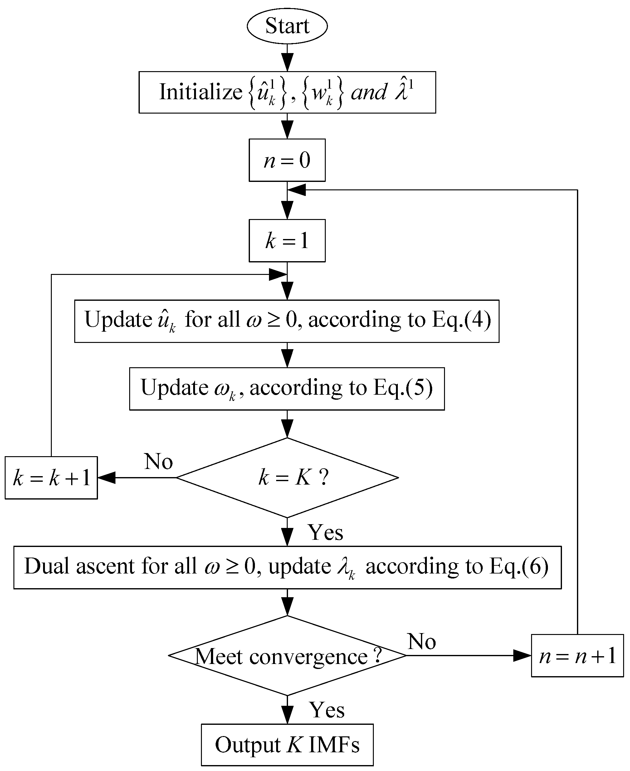
2.1. Variational Mode Decomposition (VMD)

VMD transfers the signal decomposition process into a process of solving a variational model to obtain the sub-signals (modes). It is superior to EMD in getting rid of the cycling screening signal processing method. Assuming that each mode has a limited bandwidth with a unique center frequency in the frequency domain, the signal can be adaptively decomposed by obtaining the optimal solution of the constrained variational model. The center frequency and bandwidth of each mode is constantly updated during the variational model solution process. Each mode is demodulated to its corresponding baseband, and, ultimately, all the modes and their corresponding center frequencies are extracted [25]. In the following, the process of the VMD algorithm is described briefly, and the concrete procedures involved are illustrated in Figure 1.

Figure 1. The concrete procedures of variational mode decomposition (VMD).

Figure 1. The concrete procedures of variational mode decomposition (VMD).

In the VMD algorithm, the intrinsic mode functions (IMFs) are redefined as amplitude modulated and frequency modulated (AM-FM) signals [25], which are given as a function of time t:

$$u_k(t)=A_k(t)\cos ({\mathsf{\varphi }}_k(t))$$

(1)

where ${\mathsf{\varphi }}_k(t)$ is the phase, $A_k(t)$ and ${\mathsf{\omega }}_k(t)$ are the envelope and instantaneous frequency of the kth mode $u_k(t)$, respectively, and ${\mathsf{\omega }}_k(t)$ = $\mathsf{\varphi }{\prime }_k(t)$. Both $A_k(t)$ and ${\mathsf{\omega }}_k(t)$ vary much more slowly than ${\mathsf{\varphi }}_k(t)$, which implies that, on a sufficiently long interval $[t-\mathsf{\delta },t+\mathsf{\delta }]$ ($\mathsf{\delta }\approx 2\mathsf{\pi }/\mathsf{\varphi }{\prime }_k(t)$), $u_k(t)$ can be considered to be a pure harmonic signal with amplitude $A_k(t)$ and instantaneous frequency ${\mathsf{\omega }}_k(t)$.

Assume the original signal f is decomposed into K discrete modes, such that the variational problem can be described as a constrained variational problem. The problem is targeted at minimizing the sum of the estimated bandwidth for each mode by finding K mode functions $u_k(t)$. Then the constrained variational formulation is given as follows:

$$\begin{array}{l}\underset{\left\{u_k\right\},\left\{{\mathsf{\omega }}_k\right\}}{\min }\left\{{\displaystyle \sum _k{\Vert {\partial }_t[(\mathsf{\sigma }(t)+\frac{j}{\mathsf{\pi }t})\ast u_k(t)]e^{-j{\mathsf{\omega }}_{k}t}\Vert }_2^2}\right\}\\ \mathrm{s}.\mathrm{t}.{\displaystyle \sum _k{u}_k=f}\end{array}\}$$

(2)

Here $\left\{u_k\right\}=\left\{u_1,\dots u_K\right\}$ and $\left\{{\mathsf{\omega }}_k\right\}=\left\{{\mathsf{\omega }}_1,\dots {\mathsf{\omega }}_K\right\}$ are the set of all modes and their center frequencies, respectively. $\mathsf{\sigma }(t)$ is the Dirac distribution, $j^2=-1$ and $\ast$ denotes convolution.

The above constrained variational problem can be addressed by introducing a quadratic penalty factor $\mathsf{\alpha }$ and Lagrange multipliers $\mathsf{\lambda }(t)$. Therefore, the augmented Lagrangian (L) is formulated as:

$$L(\left\{u_k\right\},\left\{{\mathsf{\omega }}_k\right\},\mathsf{\lambda })=\mathsf{\alpha }{\displaystyle \sum _k{\Vert {\partial }_t[(\mathsf{\sigma }(t)+\frac{j}{\mathsf{\pi }t})\ast u_k(t)]e^{-j{\mathsf{\omega }}_{k}t}\Vert }_2^2}+{\Vert f(t)-{\displaystyle \sum _k{u}_k(t)}\Vert }_2^2+\langle \mathsf{\lambda }(t),f(t)-{\displaystyle \sum _k{u}_k(t)}\rangle$$

(3)

where ${\Vert •\Vert }_p$ denotes the usual vector ${\ell }_p$ norm ($p=2$). The optimization methodology denoted as the alternate direction method of multipliers (ADMM) is then used to obtain the saddle point of the augmented Lagrangian by updating $u_k^{n+1}$, ${\mathsf{\omega }}_k^{n+1}$ and ${\mathsf{\lambda }}_k^{n+1}$ alternately. The convergence criterion of the algorithm is ${\displaystyle \sum _k({\Vert {\widehat{u}}_k^{n+1}-{\widehat{u}}_k^n\Vert }_2^2/{\Vert {\widehat{u}}_k^n\Vert }_2^2)<\mathsf{\epsilon }}$, where $\mathsf{\epsilon }$ is the convergence tolerance and ^ denotes the Fuorier transforms. The final updated equations are given as follows [25]:

$${\widehat{u}}_k^{n+1}(\mathsf{\omega })=\frac{\widehat{f}(\mathsf{\omega })-{\displaystyle \sum _{i<k}{\widehat{u}}_i^{n+1}(\mathsf{\omega })}-{\displaystyle \sum _{i>k}{\widehat{u}}_i^n(\mathsf{\omega })}+\frac{{\widehat{\mathsf{\lambda }}}^n(\mathsf{\omega })}{2}}{1+2\mathsf{\alpha }{(\mathsf{\omega }-{\mathsf{\omega }}_k^n)}^2}$$

(4)

$${\mathsf{\omega }}_k^{n+1}=\frac{{\displaystyle {\int }_0^{\infty }\mathsf{\omega }{\left|{\widehat{u}}_k^{n+1}(\mathsf{\omega })\right|}^{2}d\mathsf{\omega }}}{{\displaystyle {\int }_0^{\infty }{\left|{\widehat{u}}_k^{n+1}(\mathsf{\omega })\right|}^{2}d\mathsf{\omega }}}$$

(5)

$${\widehat{\mathsf{\lambda }}}^{n+1}(\mathsf{\omega })={\widehat{\mathsf{\lambda }}}^n(\mathsf{\omega })+\mathsf{\tau }[\widehat{f}(\mathsf{\omega })-{\displaystyle \sum _k{\widehat{u}}_k^{n+1}(\mathsf{\omega })}]$$

(6)

where $n$ is the iteration number and $\mathsf{\tau }$ is the time step of the dual ascent.

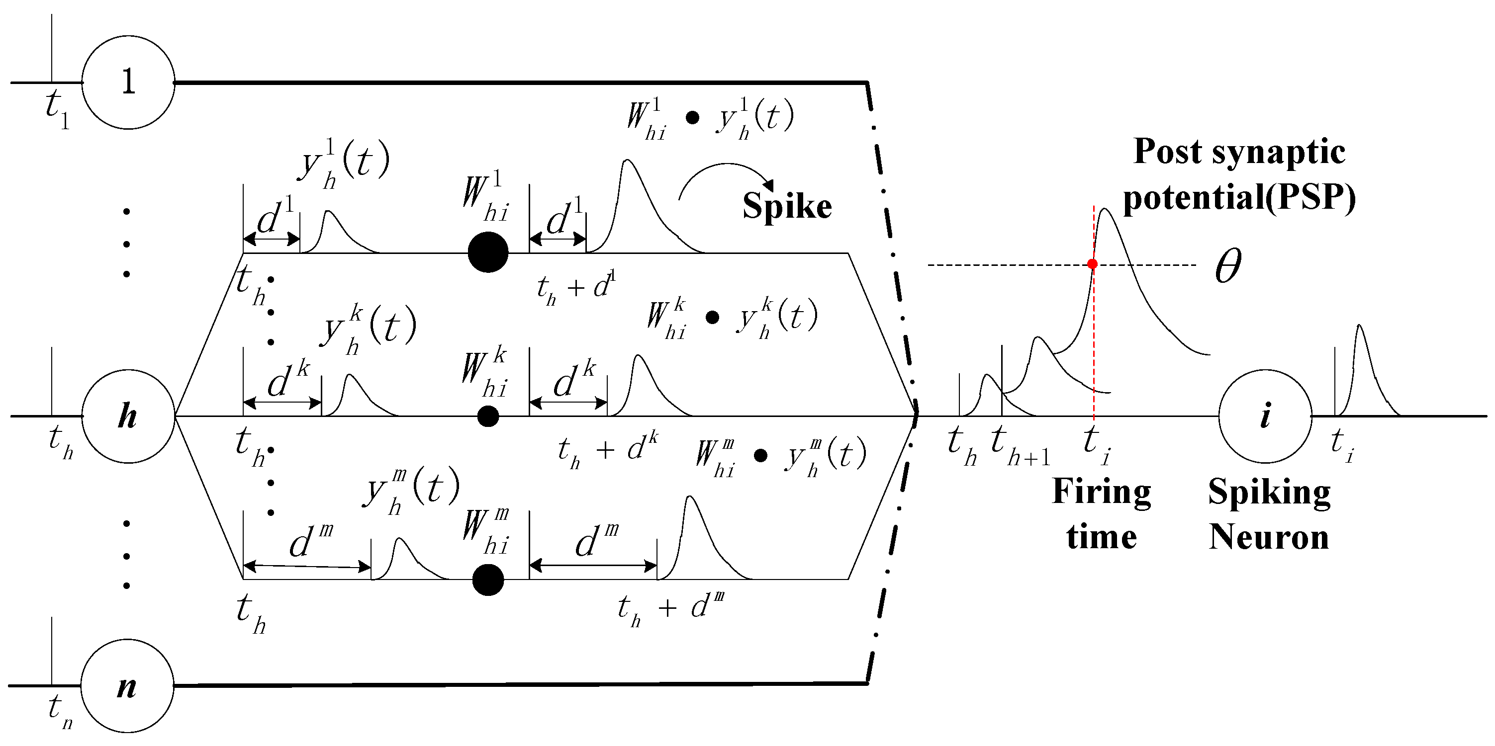
2.2. Spiking Neural Networks (SNNs)

The architecture of a SNN consists of a feedforward network of spiking neurons with multiple delayed synaptic terminals. A spiking neuron is the basic unit of a SNN, and common models of spiking neurons are the leaky integrate-and-fire model (LIFM), Hodgkin-Huxley model (HHM) and spike response model (SRM) [12]. The standard three-layer feedforward SNN based on SRM is adopted in this paper. Figure 2 illustrates the connectivity between an arbitrary spiking neuron h and the ith neuron in successive layers.

From Figure 2, we can see that the SNN differs from conventional back propagation (BP) neural network in that an individual connection consists of a fixed number of m synaptic terminals. Each terminal serves as a sub-connection associated with an adjustable delay $d^k$ and weight ${W_{hi}}^k$. A temporal encoding scheme is adopted in SNN, which takes the firing time of a spiking neuron as input and output signals directly. The characteristics of multiple delayed synaptic terminals and the time encoding scheme provide SNNs with not only a powerful computing capability and good applicability, but also time series tractability in particular.

Figure 2. The connectivity between neuron h and the ith neuron with m delayed synaptic terminals.

Figure 2. The connectivity between neuron h and the ith neuron with m delayed synaptic terminals.

Each neuron fires at most a single spike during the simulation interval, and only fires when an internal state variable, denoted as the membrane potential (MP), reaches the preset neuronal excitation threshold $\mathsf{\theta }$ (in Figure 2). Meanwhile, the neuron firing the spike generates an output signal, denoted as the post synaptic potential (PSP), which is defined by the spike-response function $\mathsf{\epsilon }(t)$:

$$\mathsf{\epsilon }(t)=\{\begin{array}{cc}\frac{t}{{\mathsf{\tau }}_s}{e}^{1-\frac{t}{{\mathsf{\tau }}_s}}\hfill & \mathrm{t}>0\hfill \\ 0\hfill & \mathrm{t}\le 0\hfill \end{array}$$

(7)

Here, ${\mathsf{\tau }}_s$ is the membrane potential decay time constant that determines the rise and decay time of the PSP. Neuron h receives a series of spikes, and its firing time is $t_h$. Therefore, the actual firing time $t_i^a$ of neuron $i$ is calculated as follows:

$$Y_h^k(t)=\mathsf{\epsilon }(t-t_h-d^k)$$

(8)

$$X_i(t)={\displaystyle \sum _h{\displaystyle \sum _{k=1}^m{W}_{hi}^k{Y}_h^k(t)}}$$

(9)

$$t_i^a:X_i(t_i^a)=\mathsf{\theta }and{\frac{d{X}_i(t)}{dt}|}_{t=t_i^a}>0$$

(10)

Here, $Y_h^k(t)$ is the unweight contribution of a single synaptic terminal to MP, and $X_i(t)$ is the MP of neuron i. $d^k$ and $W_{hi}^k$ denote the delay and weight associated with k-th synaptic terminal, respectively.

The training algorithm employed for the SNN is spike propagation (SpikeProp), which is a supervised learning algorithm proposed by Bohte et al. [14]. In the SpikeProp algorithm, the weight of the network is adjusted to minimize the training error E for the entire network until it is within an established tolerance. A detailed description of the SpikeProp algorithm for a three-layer feedforward SNN is as follows:

(1)

Calculate E for the entire network according to the difference between the actual spike firing time $t_j^a$ and the desired spike firing time $t_j^d$ of all neurons j in output layer J, respectively:

$$E=\frac{1}{2}{{\displaystyle \sum _{j\in J}\left(t_j^a-t_j^d\right)}}^2$$

(11)

(2)

Calculate ${\mathsf{\delta }}_j$ for all neurons j in output layer J:

$${\mathsf{\delta }}_j=\frac{(t_j^d-t_j^a)}{{\displaystyle \sum _{i\in {\Gamma }_j}{\displaystyle \sum _k{W}_{ij}^k\frac{\partial Y_i^k(t_j^a)}{\partial t_j^a}}}}$$

(12)

where ${\Gamma }_j$ represents the set of all presynaptic neurons for neuron j.

(3)

Calculate ${\mathsf{\delta }}_i$ for all neurons i in hidden layer I:

$${\mathsf{\delta }}_i=\frac{{\displaystyle \sum _{j\in {\Gamma }^i}{\mathsf{\delta }}_j\left\{{\displaystyle \sum _k{W}_{ij}^k\frac{\partial Y_i^k(t_j^a)}{\partial t_i^a}}\right\}}}{{\displaystyle \sum _{h\in {\Gamma }_i}{\displaystyle \sum _k{W}_{hi}^k\frac{\partial Y_h^k(t_i^a)}{\partial t_i^a}}}}$$

(13)

where ${\Gamma }^i$ and ${\Gamma }_i$ are the set of all postsynaptic neurons and presynaptic neurons for neuron i, respectively.

(4)

Adjust the weights $\Delta W_{ij}^k$ and $\Delta W_{hi}^k$ for output layer J and hidden layer I, respectively, according to the network learning rate $\mathsf{\eta }$ as follows.

$$\Delta W_{ij}^k=-\mathsf{\eta }{\mathsf{\delta }}_j{Y}_i^k\left({\mathsf{t}}_j^a\right)$$

(14)

$$\Delta W_{hi}^k=-\mathsf{\eta }{\mathsf{\delta }}_i{Y}_h^k\left({\mathsf{t}}_j^a\right)$$

(15)

3. The Proposed VMD-SNN Forecasting Model

To capture the complicated intrinsic nonlinear and non-stationary characteristics of carbon price data, by using the VMD algorithm, an original carbon price series is firstly decomposed into a series of IMF components with higher regularity than the original data. For the superior performance of SNNs in forecasting, the SNN forecasting model for each stationary IMF component is built by considering the characteristics of that component. To reflect the relationship between the input(s) and output(s) of SNNs, the PACF and the resulting partial autocorrelation graph, which is simply the plots of the PACF against the lag length, are used to determine the input variables for the SNN forecasting model corresponding to each IMF [30,31]. Finally, the forecasting results of all the IMF components are aggregated to produce a combined forecasting result for the original carbon price. A detailed description regarding the determination of input variables is given in Section 3.1, and the overall forecasting procedures are discussed in Section 3.2.

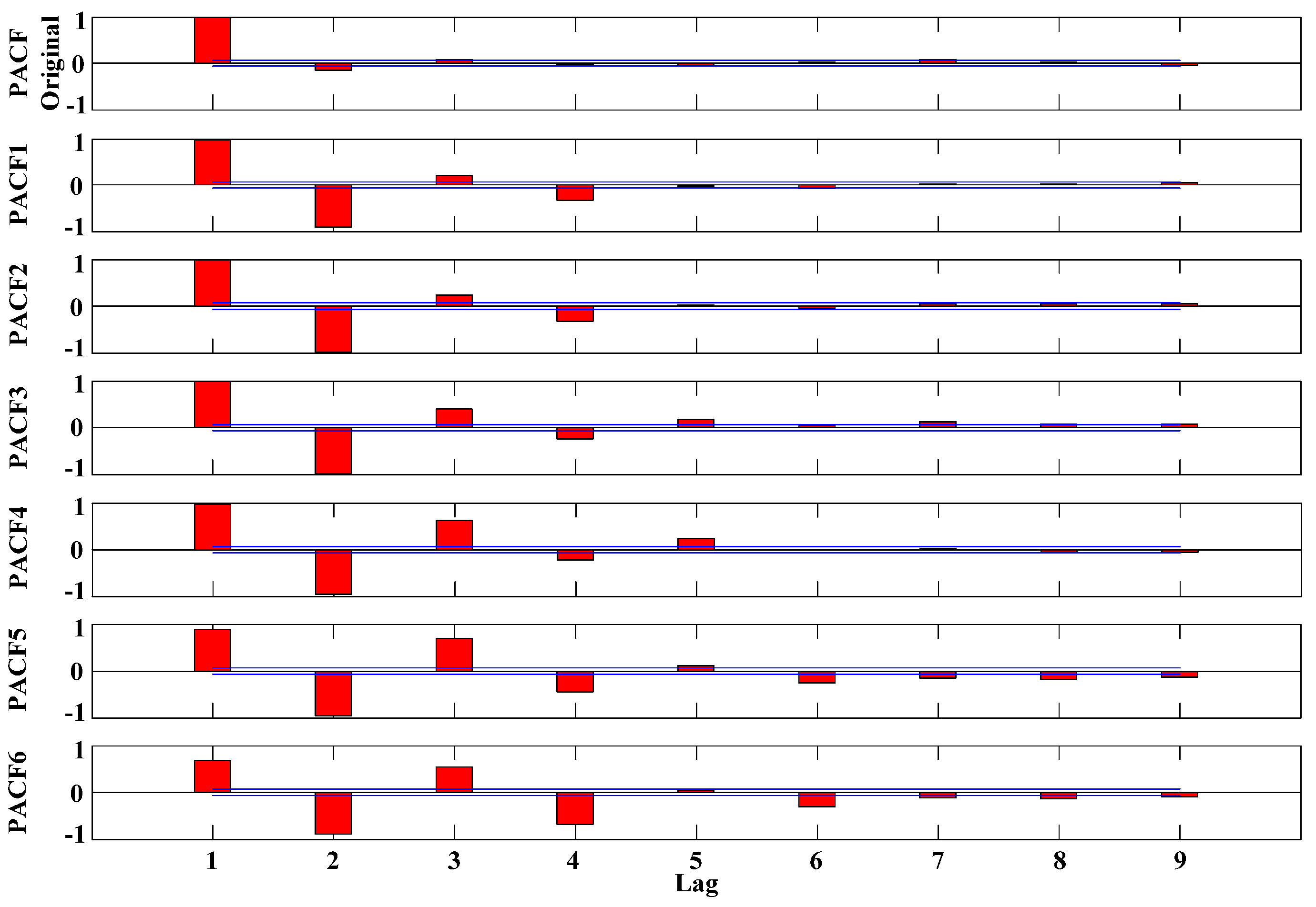
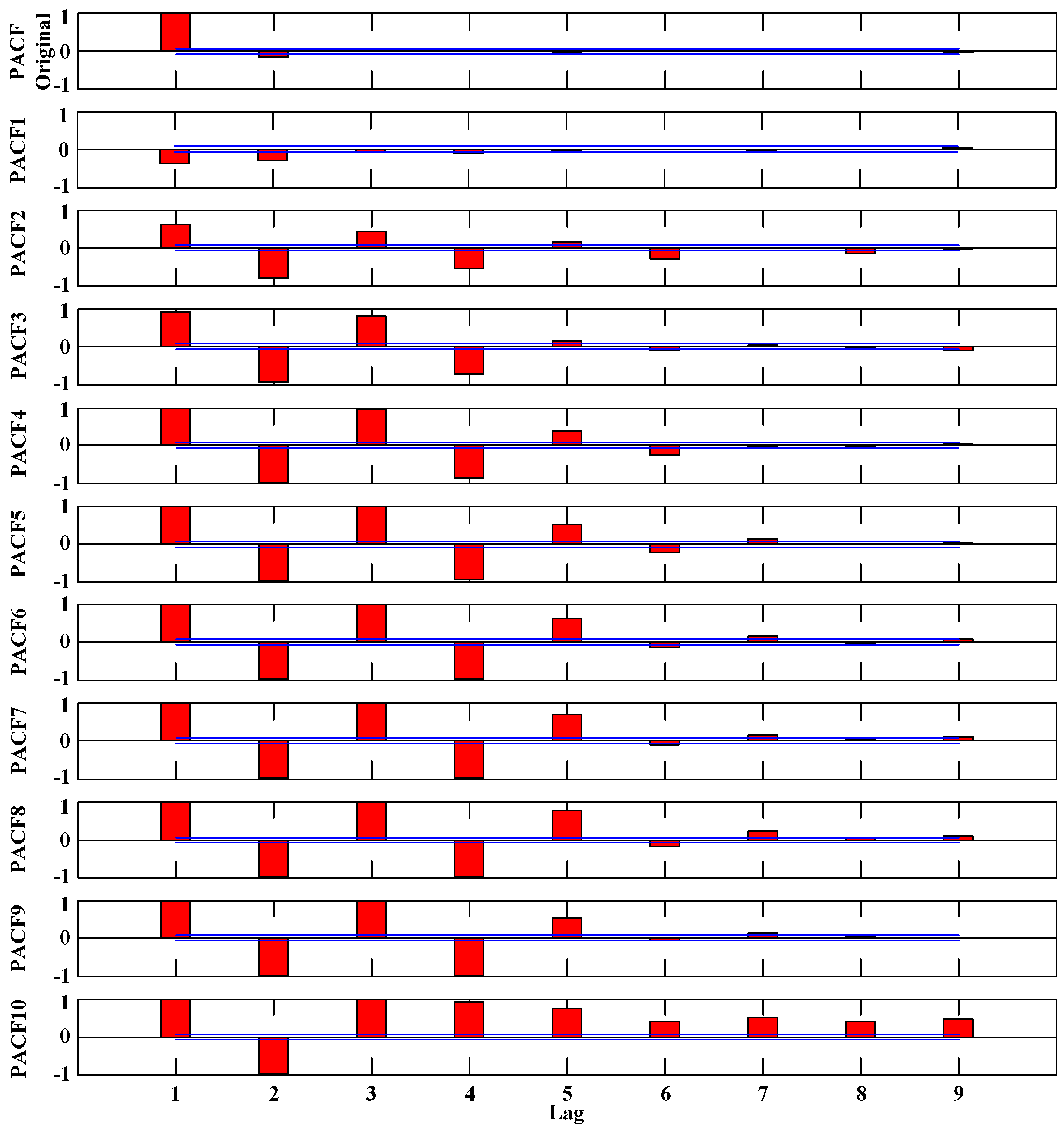
3.1. Determination of Input Variables by PACF

Assuming that $x_t$ is the output variable, if the partial autocorrelation at lag k is outside of the 95% confidence interval $[-1.96/\sqrt{N},1.96/\sqrt{N}]$, $x_{t-k}$ is one of the input variables. The previous value $x_{t-1}$ is taken as the input variable if all the PACF coefficients are within the 95% confidence interval. The PACF is described as follows: for a carbon price series $\{x_1,x_2,\cdots x_n\}$, the covariance at lag k (if k = 0, it is the variance), denoted by ${\mathsf{\gamma }}_k$, is estimated as:

$${\widehat{\mathsf{\gamma }}}_k=\frac{1}{n}{\displaystyle \sum _{t=1}^{n-k}(x_t-\overline{x})(x_{t+k}-\overline{x})},k=1,2,\dots ,M$$

(16)

where $\overline{x}$ is the mean of the carbon price series and M = n/4 is the maximum lag. Then, the autocorrelation function (ACF) at lag k, denoted by ${\mathsf{\rho }}_k$, can be estimated as:

$${\widehat{\mathsf{\rho }}}_k=\frac{{\widehat{\mathsf{\gamma }}}_k}{{\widehat{\mathsf{\gamma }}}_0}$$

(17)

Based on the covariance and the resulting ACF, the calculation for the PACF at lag k, for $k=1,2,\dots ,M$, denoted by ${\mathsf{\alpha }}_{kk}$, is presented as follows:

$$\begin{array}{c}{\widehat{\mathsf{\alpha }}}_{11}={\widehat{\mathsf{\rho }}}_1\\ {\widehat{\mathsf{\alpha }}}_{k+1,k+1}=\frac{{\widehat{\mathsf{\rho }}}_{k+1}-{\displaystyle {\sum }_{j=1}^k{\widehat{\mathsf{\rho }}}_{k+1-j}{\widehat{\mathsf{\alpha }}}_{kj}}}{1-{\displaystyle {\sum }_{j=1}^k{\widehat{\mathsf{\rho }}}_j{\widehat{\mathsf{\alpha }}}_{kj}}}\\ {\widehat{\mathsf{\alpha }}}_{k+1,j}={\widehat{\mathsf{\alpha }}}_{kj}-{\widehat{\mathsf{\alpha }}}_{k+1,k+1}\cdot {\widehat{\mathsf{\alpha }}}_{k,k-j+1},j=1,2,\dots ,k\end{array}\}$$

(18)

3.2. Overall Procedures of the VMD-SNN Forecasting Model

The overall procedures of the proposed VMD-SNN forecasting model are illustrated in Figure 3, which are generally comprised of the following main steps:

Step 1.

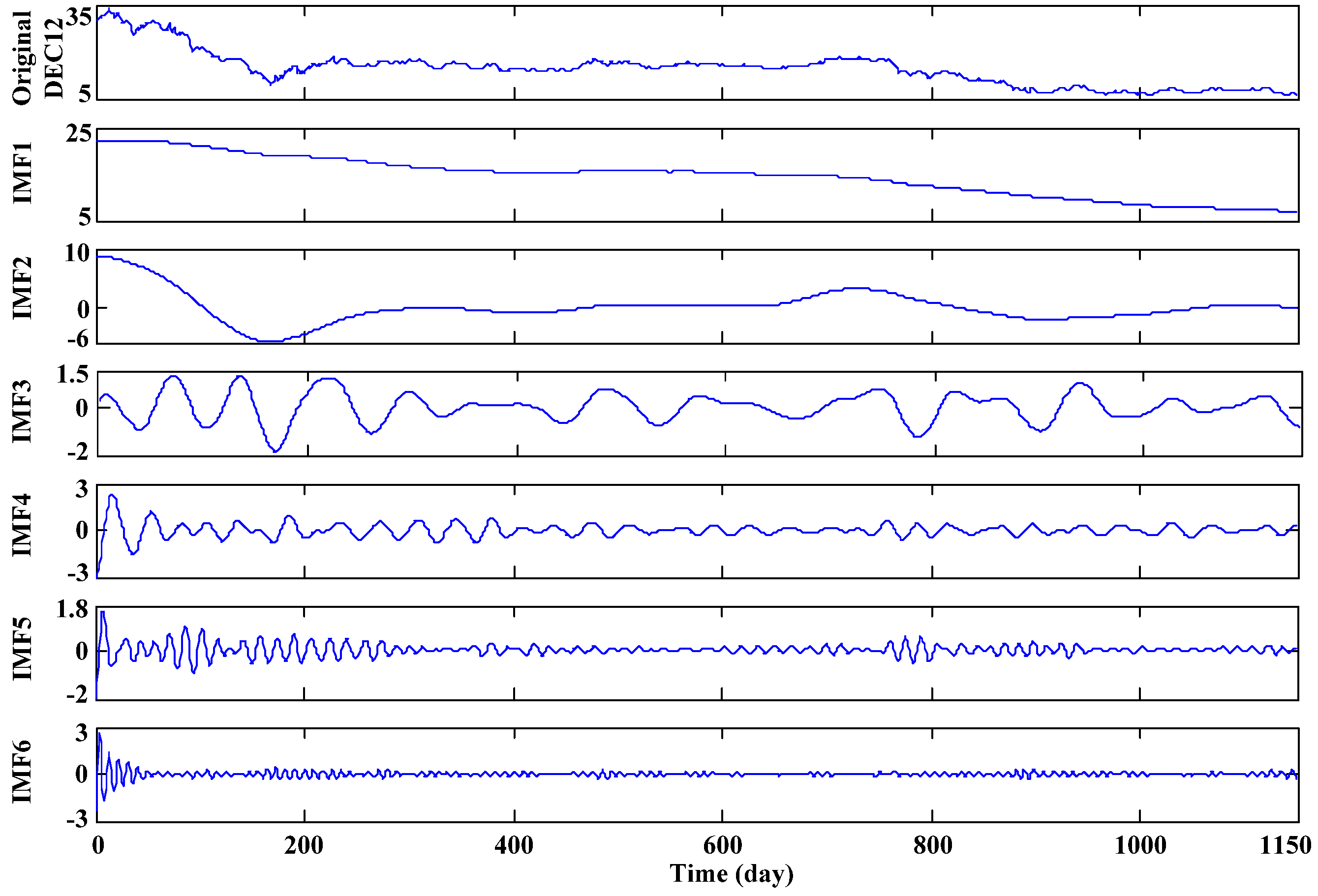
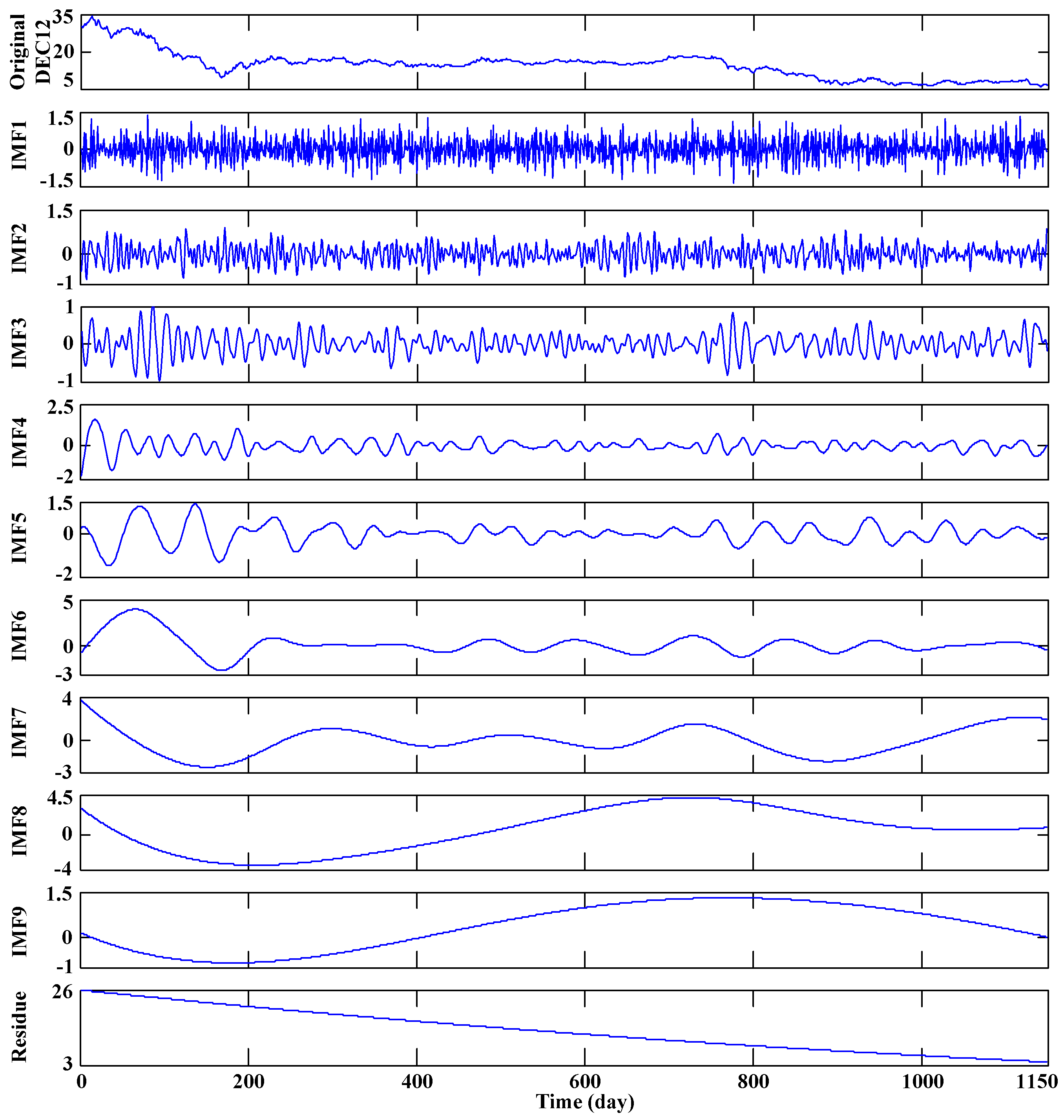
Apply the VMD algorithm to decompose the original carbon price series into K IMF components (sub-series).

Step 2.

For each IMF component, with the output variable $x_t$, the input variables are determined through observing the partial autocorrelogram via PACF.

Step 3.

A three-layer SNN forecasting model is built for each IMF component. Perform SNN training using the training sample prior to importing the test sample into the well-trained SNN model. The output is then the forecasting value of the current IMF component.

Step 4.

Aggregate the forecasting results of all the IMF components obtained by the previous steps to produce a combined forecasting result for the original carbon price series.

Step 5.

The comprehensive error evaluation criteria proposed in this paper are applied to evaluate and analyze the final forecasting result.

Figure 3. The overall procedures of the VMD-SNN forecasting model.

Figure 3. The overall procedures of the VMD-SNN forecasting model.

4. Simulation and Results Analysis

4.1. Data Description

The InterContinental Exchange (ICE) is the largest carbon emissions futures exchange in Europe. The EUA traded in the European Union emissions trading system (EU ETS) has also been leading the world carbon price, and is becoming a representative index of the general carbon price [21]. Therefore, forecasting the price of EUA carbon emissions futures matured in December, 2012 (DEC12) from the ICE can effectively reflect the overall state of the EU ETS at that time. The carbon emissions price data used in this paper are daily transaction data available from the ICE website [33].

Owing to its availability and continuity, the DEC12 carbon price series obtained from 13 June 2008 to 17 December 2012, excluding public holidays, with 1149 total data points, was chosen as experimental samples in this study. For modeling convenience, the data obtained from 13 June 2008 to 22 May 2012, excluding public holidays, with a total of 1000 data points were used as training sets, and the remaining 149 data points were used as testing sets to verify the effectiveness of the VMD-SNN forecasting model based on the comprehensive error evaluation criteria.

In addition, to improve the generalization capability and forecasting accuracy of the network, all the original carbon series and decomposed sub-series must be normalized prior to training and testing as follows:

$$p^{\ast }=\frac{p-p_{\min }}{p_{\max }-p_{\min }}$$

(19)

Here, $p^{\ast }$ represents the sample data after normalization and $p$ is the original sample data. $p_{\max }$ and $p_{\min }$ are the maximum and minimum values of p, respectively.

4.2. Comprehensive Evaluation Criteria

To evaluate the forecasting performance of the proposed VMD-SNN carbon price forecasting model comprehensively and effectively from different perspectives, this paper puts forward comprehensive evaluation criteria taking into account both level and phase errors. The level errors mainly describe the differences between actual and forecasting results in the vertical direction over a given time period. It can be often summed up as smaller or larger. The phase errors mainly describe the differences between actual and forecasting results along the horizontal timeline, which, broadly speaking reflect the leading or lagging between forecasting and actual carbon price series peaks/valleys.

4.2.1. Evaluation Indexes

Assuming that $y_i$ and ${\stackrel{⌢}{y}}_i$ are the actual and forecasting carbon price values at time i, respectively, and N is the number of data. The root mean square error (RMSE), calculated according to Equation (20), measures the degree of forecasting error dispersion, and the mean absolute error (MAE), calculated according to Equation (21), measures the average amplitude of error. Combining the two indexes can provide a macroscopic evaluation of the level error characteristics of the forecasting carbon price series. Next, the maximum absolute percentage error (MaxAPE), calculated according to Equation (22), concentrates on the maximal absolute percentage error, which reflects the forecasting risk of choosing a particular model:

$$RMSE=\sqrt{\frac{1}{N}{\displaystyle \sum _{i=1}^N{(y_i-{\stackrel{⌢}{y}}_i)}^2}},i=1,2,\cdots ,N$$

(20)

$$MAE=\frac{1}{N}{\displaystyle \sum _{i=1}^N\left|y_i-{\stackrel{⌢}{y}}_i\right|},i=1,2,\cdots ,N$$

(21)

$$MaxAPE=\underset{i}{\max }\left(\left|\frac{y_i-{\stackrel{⌢}{y}}_i}{y_i}\right|\right)\times 100,i=1,2,\cdots ,N$$

(22)

The correlation coefficient denoted by $I_{cc}$, which primarily measures the level and phase errors directly, can describe the correlation between the actual and forecasting carbon price series. The forecasting accuracy increases with increasing $I_{cc}$, and is defined as follows:

$$I_{cc}=\frac{\mathrm{cov}(Y_a,Y_f)}{\sqrt{\mathrm{D}{Y}_a}\sqrt{\mathrm{D}{Y}_f}}$$

(23)

where $Y_a$ and $Y_f$ are the actual and forecasting carbon price series, respectively, and D represents the variance.

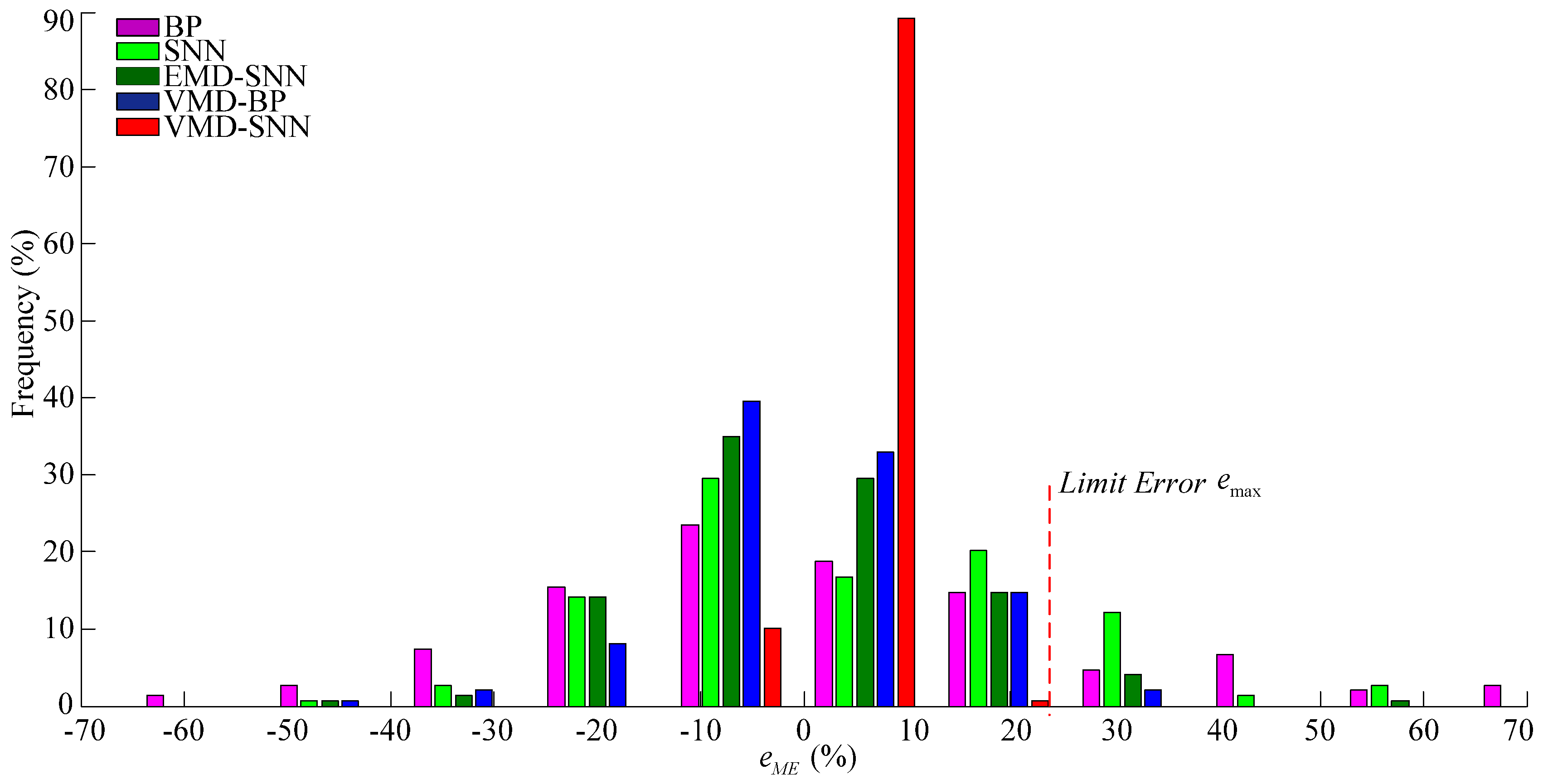
4.2.2. Histogram of the Error Frequency Distribution

This index is an improvement of the mean error (ME), which substitutes the original averaging process for the form of frequency distribution histogram. This index reserves the function of ME to measure whether the system is unbiased, in addition, it gives distribution of the error bands in the forecasting result. The degree of concentration for the error frequency distribution relative to zero can be regarded as a basis for comparing different forecasting models.

4.3. Parameter Setting

To demonstrate the effectiveness of the proposed VMD-SNN forecasting model, the single BP and SNN models are employed as benchmarks for comparison. In addition, the combined EMD-SNN and VMD-BP models are also used to forecast the carbon price for the purpose of comparison. The forecasting simulations are performed on a MATLAB^® (R2014a) platform, and the simulation parameters are set as follows.

The number of modes K should be firstly determined when applying the VMD algorithm to decompose the original DEC12 carbon price series. The primary distinguishing characteristic of a mode is its center frequency. Thus, for simplicity, we determined K on the basis of the method’s capability to distinguish center frequencies. For DEC12, modes with similar center frequencies are observed to appear when K reaches 6, and we argue that this corresponds with the onset of greedy decomposition. Consequently, K is set to 6. The penalty factor $\mathsf{\alpha }$ and the tolerance of convergence criterion $\mathsf{\epsilon }$ are set to default values of 2000 and ${10}^{-6}$, respectively. Moreover, the noise with low level in the original data can be filtered by adjusting the update parameter $\mathsf{\tau }>0$, and the value is set to 0.3 in this paper. For the EMD algorithm, the thresholds and tolerance level of the stop criterion are determined as $\left[{\mathsf{\theta }}_1,{\mathsf{\theta }}_1,\mathsf{\alpha }\right]=\left[0.05,0.5,5\times {10}^{-4}\right]$.

In the SNN model, the number of synaptic terminals m is set to 16, and the corresponding synapses delay $d^k$ is selected as an incremental integer in the interval [1,16]. The decay time constant ${\mathsf{\tau }}_s$ is set to 6 ms, and the excitation threshold $\mathsf{\theta }$ for all neurons is set as 1 mV. For both SNN and BP, the maximum iterations and learning rate are set as 1000 and 0.0005, respectively.

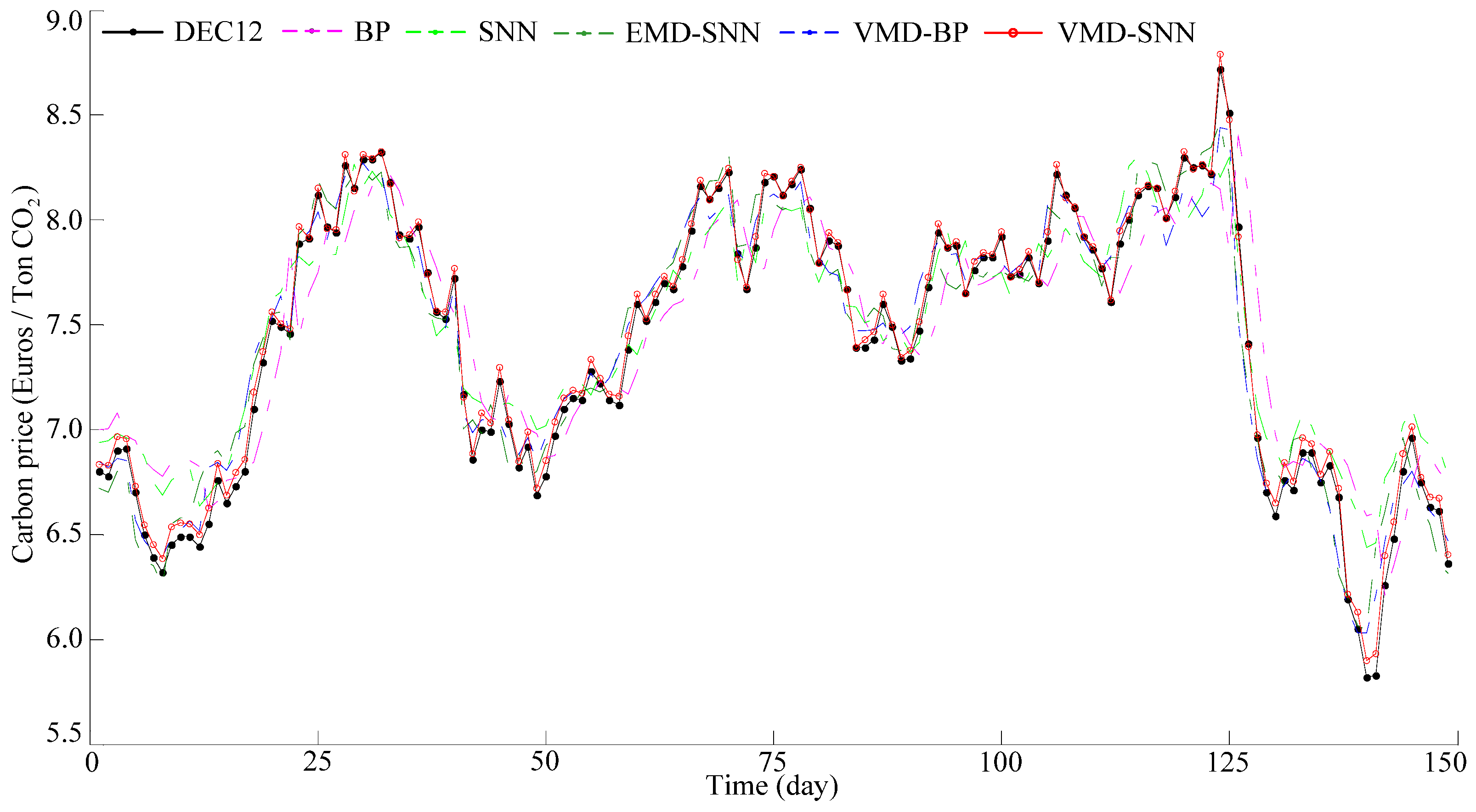
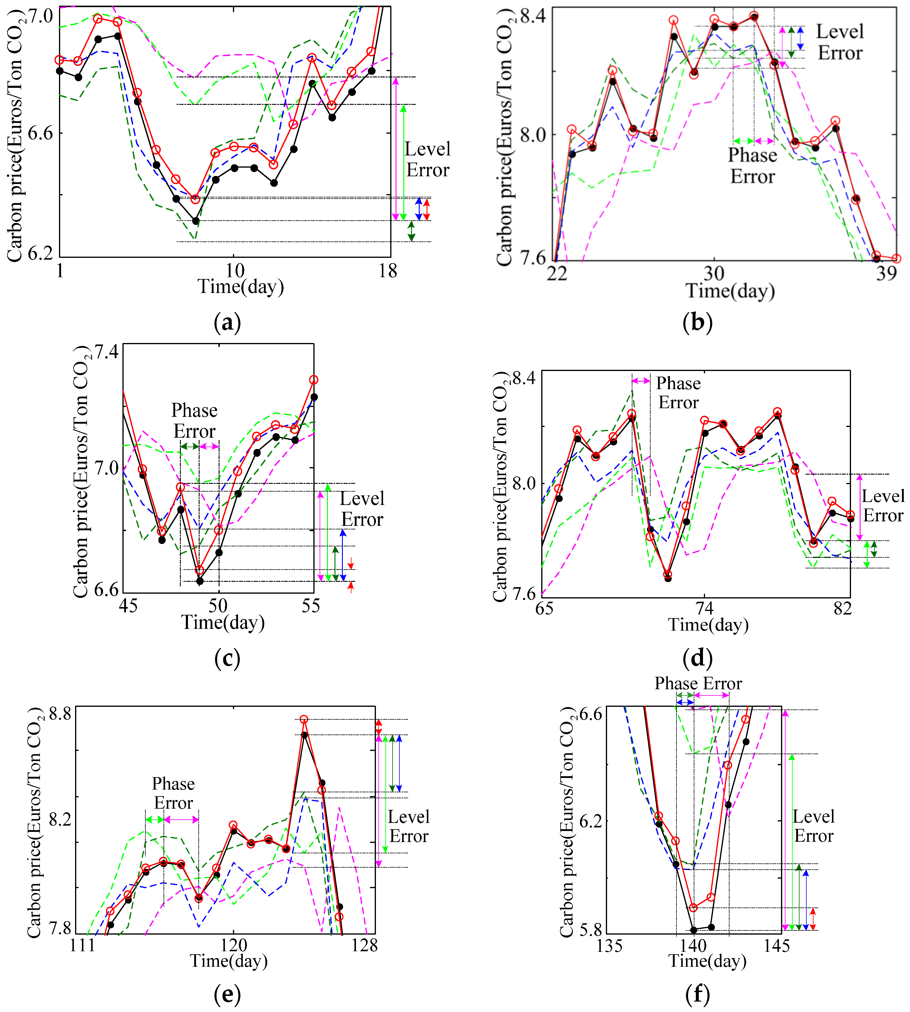
4.4. Results and Analysis

The forecasting simulations are conducted according to the procedures discussed in Section 3.2. Firstly, the proposed VMD algorithm and the widely used EMD algorithm are adopted to decompose the DEC12 carbon price series, and the decomposition results are illustrated in Figure 4 and Figure 5, respectively.

Figure 4. The decomposition of DEC12 using the VMD algorithm.

Figure 4. The decomposition of DEC12 using the VMD algorithm.

Figure 5. The decomposition of DEC12 using the EMD algorithm.

Figure 5. The decomposition of DEC12 using the EMD algorithm.

Based on Figure 4 and Figure 5, it can be observed that the original DEC12 series is decomposed into six IMFs via VMD and nine IMFs plus one residue via EMD. It is noteworthy that, although the carbon price is positive, the values of IMFs may be negative.

The VMD algorithm extracts the significant volatility and trend sub-series at equivalent scales in the original DEC12. In addition, relative to the IMFs derived from VMD, the values of IMF1–IMF3 derived from EMD oscillate with very high frequencies, which results in additional difficulties for forecasting. Then, using the PACF, the partial autocorrelogram of DEC12 and the obtained IMFs can be conveniently derived, which are shown in Figure 6 and Figure 7, respectively. Based on evaluation of the partial autocorrelograms, the input variables of the original carbon price series and the IMFs obtained via the two decomposition algorithms corresponding to output variable $x_t$ are presented in Table 1.

Figure 6. The PACFs of the original series and the IMFs derived from VMD.

Figure 6. The PACFs of the original series and the IMFs derived from VMD.

Figure 7. The PACFs of the original series and the IMFs derived from EMD.

Figure 7. The PACFs of the original series and the IMFs derived from EMD.

Table 1. Input variables of the original series and the IMFs.

Series	Mode Decomposition Algorithm
	VMD	EMD
DEC12	$(x_{t-1},x_{t-2},x_{t-3},x_{t-7})$	$(x_{t-1},x_{t-2},x_{t-3},x_{t-7})$
IMF1	$(x_{t-1},x_{t-2},x_{t-3},x_{t-4},x_{t-6})$	$(x_{t-1},x_{t-2},x_{t-3},x_{t-4})$
IMF2	$(x_{t-1},x_{t-2},x_{t-3},x_{t-4})$	$(x_{t-1},x_{t-2},x_{t-3},x_{t-4},x_{t-5},x_{t-6},x_{t-8})$
IMF3	$(x_{t-1},x_{t-2},x_{t-3},x_{t-4},x_{t-5},x_{t-7},x_{t-8},x_{t-9})$	$(x_{t-1},x_{t-2},x_{t-3},x_{t-4},x_{t-5},x_{t-6},x_{t-8},x_{t-9})$
IMF4	$(x_{t-1},x_{t-2},x_{t-3},x_{t-4},x_{t-5},x_{t-9})$	$(x_{t-1},x_{t-2},x_{t-3},x_{t-4},x_{t-5},x_{t-6})$
IMF5	$(x_{t-1},x_{t-2},x_{t-3},x_{t-4},x_{t-5},x_{t-6},x_{t-7},x_{t-8},x_{t-9})$	$(x_{t-1},x_{t-2},x_{t-3},x_{t-4},x_{t-5},x_{t-6},x_{t-7})$
IMF6	$(x_{t-1},x_{t-2},x_{t-3},x_{t-4},x_{t-6},x_{t-7},x_{t-8},x_{t-9})$	$(x_{t-1},x_{t-2},x_{t-3},x_{t-4},x_{t-5},x_{t-6},x_{t-7})$
IMF7	—	$(x_{t-1},x_{t-2},x_{t-3},x_{t-4},x_{t-5},x_{t-6},x_{t-7},x_{t-9})$
IMF8	—	$(x_{t-1},x_{t-2},x_{t-3},x_{t-4},x_{t-5},x_{t-6},x_{t-7},x_{t-9})$
IMF9	—	$(x_{t-1},x_{t-2},x_{t-3},x_{t-4},x_{t-5},x_{t-7},x_{t-9})$
Residue	—	$(x_{t-1},x_{t-2},x_{t-3},x_{t-4},x_{t-5},x_{t-6},x_{t-7},x_{t-8},x_{t-9})$

Table 1. Input variables of the original series and the IMFs.

Series	Mode Decomposition Algorithm
	VMD	EMD
DEC12	$(x_{t-1},x_{t-2},x_{t-3},x_{t-7})$	$(x_{t-1},x_{t-2},x_{t-3},x_{t-7})$
IMF1	$(x_{t-1},x_{t-2},x_{t-3},x_{t-4},x_{t-6})$	$(x_{t-1},x_{t-2},x_{t-3},x_{t-4})$
IMF2	$(x_{t-1},x_{t-2},x_{t-3},x_{t-4})$	$(x_{t-1},x_{t-2},x_{t-3},x_{t-4},x_{t-5},x_{t-6},x_{t-8})$
IMF3	$(x_{t-1},x_{t-2},x_{t-3},x_{t-4},x_{t-5},x_{t-7},x_{t-8},x_{t-9})$	$(x_{t-1},x_{t-2},x_{t-3},x_{t-4},x_{t-5},x_{t-6},x_{t-8},x_{t-9})$
IMF4	$(x_{t-1},x_{t-2},x_{t-3},x_{t-4},x_{t-5},x_{t-9})$	$(x_{t-1},x_{t-2},x_{t-3},x_{t-4},x_{t-5},x_{t-6})$
IMF5	$(x_{t-1},x_{t-2},x_{t-3},x_{t-4},x_{t-5},x_{t-6},x_{t-7},x_{t-8},x_{t-9})$	$(x_{t-1},x_{t-2},x_{t-3},x_{t-4},x_{t-5},x_{t-6},x_{t-7})$
IMF6	$(x_{t-1},x_{t-2},x_{t-3},x_{t-4},x_{t-6},x_{t-7},x_{t-8},x_{t-9})$	$(x_{t-1},x_{t-2},x_{t-3},x_{t-4},x_{t-5},x_{t-6},x_{t-7})$
IMF7	—	$(x_{t-1},x_{t-2},x_{t-3},x_{t-4},x_{t-5},x_{t-6},x_{t-7},x_{t-9})$
IMF8	—	$(x_{t-1},x_{t-2},x_{t-3},x_{t-4},x_{t-5},x_{t-6},x_{t-7},x_{t-9})$
IMF9	—	$(x_{t-1},x_{t-2},x_{t-3},x_{t-4},x_{t-5},x_{t-7},x_{t-9})$
Residue	—	$(x_{t-1},x_{t-2},x_{t-3},x_{t-4},x_{t-5},x_{t-6},x_{t-7},x_{t-8},x_{t-9})$

After determining the input variables, basic single BP and SNN models are used to forecast the original carbon price series and the obtained IMFs. Meanwhile, the forecasting results of the IMFs were aggregated to produce a combined forecasting result for the VMD-based and EMD-based modeling processes, respectively. The actual DEC12 carbon price series and the final forecasting results of various forecasting models are presented in Figure 8. In addition, to facilitate comparison, enlarged views of the carbon price series curves shown in Figure 8 in the time intervals reflecting strong volatility are given in Figure 9. Enlarged views basically cover the peaks and valleys of the actual DEC12 carbon price series curve, and can reflect the fluctuation characteristics of the DEC12 and the tracking performance of forecasting models.

It follows from the DEC12 data shown in Figure 8 that, despite the periodic volatility at different scales, an abnormal stochastic volatility is observed in the carbon price series. Therefore, the complexity of the carbon price variation makes accurate forecasting difficult. Nevertheless, the forecasting result of the proposed VMD-SNN model closely tracks the changing trends of the actual carbon price, even nearby inflection points, which is made particularly apparent from Figure 9 under conditions of extreme price volatility. The tracking performances of the other forecasting models considered in this paper are obviously inferior. For example, the forecasting results of single BP and SNN models exhibit large level errors in time interval [1,18], [111,128], [45,55] and [135,145]. On the other hand, large phase errors exist in the forecasting results of the combined EMD-SNN and VMD-BP models in time interval [135,145].

Figure 8. Actual carbon price and the forecasting results of various models.

Figure 8. Actual carbon price and the forecasting results of various models.

Figure 9. Enlarged views of the carbon price series curves in the time interval: (a) [1,18]; (b) [22,39]; (c) [45,55]; (d) [65,82]; (e) [111,128]; (f) [135,145].

Figure 9. Enlarged views of the carbon price series curves in the time interval: (a) [1,18]; (b) [22,39]; (c) [45,55]; (d) [65,82]; (e) [111,128]; (f) [135,145].

For a quantitative analysis of the forecasting results, Table 2 lists the error statistics for the various forecasting models considered. In Table 2, the RMSE, MAE, MaxAPE and $I_{cc}$ values of the VMD-SNN model are 0.0437, 0.0355, 2.197% and 0.9993, respectively, indicating that the forecasting accuracy is higher and the forecasting risk is smaller when using the proposed VMD-SNN model to forecast the carbon price. Based on Table 2, we can further conclude the following: (a) The forecasting performance of the single SNN model is better than that of the conventional BP model, which indicates that SNN is more capable of strong nonlinear mapping, and is more applicable to forecasting the dynamic and nonlinear characteristics of the carbon price; (b) The forecasting performances of the combined forecasting models are superior to any single model. This may be attributable to the fact that mode decomposition can capture the complicated intrinsic characteristics, including both linear and nonlinear characteristics, in the carbon price series. Therefore, integrating a mode decomposition method within forecasting models has a positive effect on the overall forecasting capability; (c) That the proposed VMD-SNN forecasting model outperforms the EMD-SNN model can be mainly attributed to the fact that the carbon price series is decomposed more accurately via the VMD algorithm. This emphasizes the significance of the VMD algorithm for improving forecasting performance in carbon price forecasting.

Table 2. Error statistics for various forecasting models.

Evaluation Indexes	Forecasting Models
	BP	SNN	EMD-SNN	VMD-BP	VMD-SNN
RMSE	0.2655	0.2077	0.1528	0.1231	0.0437
MAE	0.2062	0.1690	0.1220	0.0955	0.0355
MaxAPE (%)	13.239	10.827	10.546	6.495	2.197
$I_{cc}$	0.9180	0.9621	0.9709	0.9822	0.9993

Table 2. Error statistics for various forecasting models.

Evaluation Indexes	Forecasting Models
	BP	SNN	EMD-SNN	VMD-BP	VMD-SNN
RMSE	0.2655	0.2077	0.1528	0.1231	0.0437
MAE	0.2062	0.1690	0.1220	0.0955	0.0355
MaxAPE (%)	13.239	10.827	10.546	6.495	2.197
$I_{cc}$	0.9180	0.9621	0.9709	0.9822	0.9993

Figure 10 shows histograms of the error frequency distribution for the various forecasting models considered. The frequency with which the forecasting error $e_{ME}\%$ of the proposed VMD-SNN model resides within the interval (0, 10%) is approximately 90%. It is obvious that the range of error distribution of the proposed VMD-SNN model is very narrow, and the degree of concentration for the error frequency distribution relative to zero is much greater than that of the other forecasting models. Moreover, the limit error of the VMD-SNN model is slightly greater than 20%, which is far smaller than that of the other models. The above analysis implies that the proposed VMD-SNN model yields significant improvements in carbon price forecasting.

Figure 10. Histograms of the error frequency distribution for the various forecasting models.

Figure 10. Histograms of the error frequency distribution for the various forecasting models.

5. Conclusions

Carbon price forecasting is a difficult and complex task owing to the non-linear and non-stationary characteristics of carbon price series data. It is scarcely possible to achieve a satisfactory forecasting result by simply employing a single model. This paper focused on aggregating multi-algorithms to exploit the intrinsic characteristics of carbon price series data, and a VMD-SNN combined forecasting model was proposed to forecast the carbon price. Using VMD, the carbon price series is decomposed into volatility and trend sub-series at equivalent scales, such that the complicated intrinsic linear and nonlinear characteristics are appropriately captured. The SNN model, which is capable of strong nonlinear mapping, is proposed as a forecaster for each decomposition component. Additionally, the PACF and the partial autocorrelogram are used as statistical tools to determine the input variables for the resulting SNN forecasting models. The individual results are aggregated to produce a final forecasting result for the original carbon price series. The actual daily transaction price data of EUA from the ICE obtained from 13 June 2008 to 22 May 2012 is used to verify the effectiveness of the proposed VMD-SNN forecasting model, and quantitative evaluation is conducted based on comprehensive error evaluation criteria. Simulation results and analysis demonstrate that the influence of nonlinear and non-stationary characteristics of data on the carbon price forecasting is reduced by the VMD-SNN model. Therefore the proposed VMD-SNN combined forecasting model performs better than conventional single models and EMD-based combined models. The simulation results also suggest that the model not only can be used to forecast the carbon price, but also can be extensively applied to other forecasting fields.

References

1. Alberola, E.; Chevallier, J.; Chèze, B. Price drivers and structural breaks in European carbon price 2005–2007. Energy Policy 2008, 36, 787–797. [Google Scholar] [CrossRef]
2. Liu, Y.; Huang, G.; Cai, Y. An inexact mix-integer two-stage linear programming model for supporting the management of a low-carbon energy system in China. Energies 2011, 4, 1657–1686. [Google Scholar] [CrossRef]
3. Yang, J.; Feng, X.; Tang, Y. A power system optimal dispatch strategy considering the flow of carbon emissions and large consumers. Energies 2015, 8, 9087–9106. [Google Scholar] [CrossRef]
4. Zhu, Y.; Li, Y.P.; Huang, G.H. A dynamic model to optimize municipal electric power systems by considering carbon emission trading under uncertainty. Energy 2015, 88, 636–649. [Google Scholar] [CrossRef]
5. Chevallier, J. Carbon futures and macroeconomic risk factors: A view from the EU ETS. Energy Econ. 2009, 31, 614–625. [Google Scholar] [CrossRef]
6. Wang, Y.; Wu, C. Forecasting energy market volatility using GARCH models: Can multivariate models beat univariate models? Energy Econ. 2012, 34, 2167–2181. [Google Scholar] [CrossRef]
7. Tsai, M.T.; Kuo, Y.T. A forecasting system of carbon price in the carbon trading markets using artificial neural network. Int. J. Environ. Sci. Dev. 2013, 4, 163–167. [Google Scholar] [CrossRef]
8. Zhu, B.; Wang, P.; Chevallier, J. Carbon price analysis using empirical mode decomposition. Comput. Econ. 2014, 45, 195–206. [Google Scholar] [CrossRef]
9. Zhu, B. A novel multiscale combined carbon price prediction model integrating empirical mode decomposition, genetic algorithm and artificial neural network. Energies 2012, 5, 355–370. [Google Scholar] [CrossRef]
10. Li, W.; Lu, C. The research on setting a unified interval of carbon price benchmark in the national carbon trading market of China. Appl. Energy 2015, 155, 728–739. [Google Scholar] [CrossRef]
11. Maass, W. Networks of spiking neurons: The third generation of neural network models. Neural Netw. 1997, 10, 1659–1671. [Google Scholar] [CrossRef]
12. Gerstner, W.; Kistler, W.M. Spiking Neuron Models: Single Neurons, Populations, Plasticity; Cambridge University Press: Cambridge, UK, 2002. [Google Scholar]
13. Ponulak, F.; Kasinski, A. Introduction to spiking neural networks: Information processing, learning and applications. Acta Neurobiol. Exp. 2010, 71, 409–433. [Google Scholar]
14. Bohte, S.M.; Kok, J.N.; La-Poutre, H. Error-backpropagation in temporally encoded networks of spiking neurons. Neurocomputing 2002, 48, 17–37. [Google Scholar] [CrossRef]
15. Rowcliffe, P.; Feng, J. Training spiking neuronal networks with applications in engineering tasks. IEEE Trans. Neural Netw. 2008, 19, 1626–1640. [Google Scholar] [CrossRef] [PubMed]
16. Ghosh-Dastidar, S.; Adeli, H. Improved spiking neural networks for EEG classification and epilepsy and seizure detection. Integr. Comput. Aided Eng. 2007, 14, 187–212. [Google Scholar]
17. Kulkarni, S.; Simon, S.P.; Sundareswaran, K. A spiking neural network (SNN) forecast engine for short-term electrical load forecasting. Appl. Soft Comput. 2013, 13, 3628–3635. [Google Scholar] [CrossRef]
18. Sharma, V.; Srinivasan, D. A spiking neural network based on temporal encoding for electricity price time series forecasting in deregulated markets. In Proceedings of the 2010 IEEE International Joint Conference on Neural Networks (IJCNN), Barcelona, Spain, 18–23 July 2010.
19. Lin, Y.; Teng, Z.J. Prediction of grain yield based on spiking neural networks model. In Proceedings of the 3rd IEEE International Conference on Communication Software and Networks (ICCSN), Xi’an, China, 27–29 May 2011.
20. Seifert, J.; Uhrig-Homburg, M.; Wagner, M. Dynamic behavior of CO2 spot price. J. Environ. Econ. Manag. 2008, 56, 180–194. [Google Scholar] [CrossRef]
21. Zhang, Y.J.; Wei, Y.M. An overview of current research on EU ETS: Evidence from its operating mechanism and economic effect. Appl. Energy 2010, 87, 1804–1814. [Google Scholar] [CrossRef]
22. Huang, N.E.; Shen, Z.; Long, S.R.; Wu, M.C.; Shih, H.H.; Zheng, Q.; Yen, N.C.; Tung, C.C.; Liu, H.H. The empirical mode decomposition and the Hilbert spectrum for nonlinear and nonstationary time series analysis. Proc. R. Soc. Lond. A 1998, 454, 903–995. [Google Scholar] [CrossRef]
23. Hong, Y.Y.; Yu, T.H.; Liu, C.Y. Hour-ahead wind speed and power forecasting using empirical mode decomposition. Energies 2013, 6, 6137–6152. [Google Scholar] [CrossRef]
24. Fan, G.F.; Qing, S.; Wang, H. Support vector regression model based on empirical mode decomposition and auto regression for electric load forecasting. Energies 2013, 6, 1887–1901. [Google Scholar] [CrossRef]
25. Dragomiretskiy, K.; Zosso, D. Variational mode decomposition. IEEE Trans. Signal Proc. 2014, 62, 531–544. [Google Scholar] [CrossRef]
26. Upadhyay, A.; Pachori, R.B. Instantaneous voiced/non-voiced detection in speech signals based on variational mode decomposition. J. Frankl. Inst. 2015, 352, 2679–2707. [Google Scholar] [CrossRef]
27. Lahmiri, S. Long memory in international financial markets trends and short movements during 2008 financial crisis based on variational mode decomposition and detrended fluctuation analysis. Phys. A Stat. Mech. Appl. 2015, 437, 130–138. [Google Scholar] [CrossRef]
28. Aneesh, C.; Kumar, S.; Hisham, P.M. Performance comparison of variational mode decomposition over empirical wavelet transform for the classification of power quality disturbances using support vector machine. Procedia Comput. Sci. 2015, 46, 372–380. [Google Scholar] [CrossRef]
29. Wang, Y.; Markert, R.; Xiang, J. Research on variational mode decomposition and its application in detecting rub-impact fault of the rotor system. Mech. Syst. Signal Proc. 2015, 60, 243–251. [Google Scholar] [CrossRef]
30. Dégerine, S.; Lambert-Lacroix, S. Characterization of the partial autocorrelation function of nonstationary time series. J. Multivar. Anal. 2003, 87, 46–59. [Google Scholar] [CrossRef]
31. Guo, Z.; Zhao, W.; Lu, H. Multi-step forecasting for wind speed using a modified EMD-based artificial neural network model. Renew. Energy 2012, 37, 241–249. [Google Scholar]
32. Giebel, G.; Brownsword, R.; Kariniotakis, G. The State-of-the-Art in Short-Term Prediction of Wind Power: A Literature Overview, 2nd ed.; ANEMOS. Plus: Risoe DTU, Roskilde, Denmark, 2011. [Google Scholar]
33. ICE EUA Futures Contract: Historic Data 2008-2012. Available online: http://www.theice.com (accessed on 24 December 2014).