Article

Accelerated Model Predictive Control for Electric Vehicle Integrated Microgrid Energy Management: A Hybrid Robust and Stochastic Approach

1
School of Electrical Engineering, Southeast University, Nanjing 210096, China
2
Jiangsu Key Laboratory of Smart Grid Technology and Equipment, Nanjing 210096, China
3
Electric Power Research Institute, State Grid Jiangsu Power Supply Company, Nanjing 211103, China
*
Author to whom correspondence should be addressed.
Energies 2016, 9(11), 973; https://doi.org/10.3390/en9110973
Submission received: 25 October 2016 / Revised: 15 November 2016 / Accepted: 17 November 2016 / Published: 22 November 2016
(This article belongs to the Special Issue Smart Microgrids: Developing the Intelligent Power Grid of Tomorrow)

Abstract

:
A microgrid with an advanced energy management approach is a feasible solution for accommodating the development of distributed generators (DGs) and electric vehicles (EVs). At the primary stage of development, the total number of EVs in a microgrid is fairly small but increases promptly. Thus, it makes most prediction models for EV charging demand difficult to apply at present. To overcome the inadaptability, a novel robust approach is proposed to handle EV charging demand predictions along with demand-side management (DSM) on the condition of satisfying each EV user’s demand. Variables with stochastic forecast models join the objective function in the form of probability-constrained scenarios. This paper proposes a scenario-based model predictive control (MPC) approach combining both robust and stochastic models to minimize the total operational cost for energy management. To overcome the concern about the convergence time increasing from the combination of scenarios, the Benders decomposition (BD) technique is further adopted to improve computational efficiency. Simulation results on a combined heat and power microgrid indicate that the proposed scenario-based MPC approach achieves a better economic performance than a traditional deterministic MPC (DMPC) approach, while ensuring EV charging demands, as well as minimizing the trade-off between optimal solutions and computing times.

1. Introduction

Introduced to streamline the operation of increasing penetration of distributed generations (DGs) in distribution networks, microgrids are capable of providing a systematic scheme to integrate local dispatchable DGs, such as combined heat and power (CHP) units, renewable energy systems (RESs), energy storage systems (ESSs), electric vehicles (EVs), and require intelligent energy management systems subject to some criteria, such as economic performance, user satisfaction, reliability, etc. [1,2]. Energy management approaches are complex tasks which require dynamic assessment of current and future operations while considering time-varying energy consumption, production, and prices [3,4,5]. Meanwhile, by treating EV charging requests as postponable electrical loads under some appropriate demand-side management (DSM) strategies, the energy management of microgrids can be more flexible and cost-effective [6,7].
A promising domain for energy management is methods related to model predictive control (MPC). Being one of the most well-developed control techniques in the process industry, MPC deals with multiple-input-multiple-output systems quite well, and strong attention has been paid to its potential of reducing the operational costs of microgrids [8]. The MPC-based approaches employ a receding horizon strategy, which keeps the total operational cost low without violating the supply-demand balance and the pre-defined operation constraints. Prediction models for variables related to microgrids, such as RES outputs, real-time energy prices, load demands, etc., make it possible to implement MPC into energy management. While explicit prediction models have been used over a deterministic MPC (DMPC) approach, uncertainty models conveying detailed information about variable forecasts have drawn more attention lately. Two uncertainty models have been successfully integrated into MPC, namely robust models and stochastic models. Robust models treat uncertainties as one set-bounded scenario irrespective of scenario probabilities, providing rapid but conservative decisions while ensuring the robustness of the optimization when prediction models are not effective enough [9]. Stochastic models minimize the expected value of the objective function considering the probability-constrained scenarios of predictions, but are usually associated with large volumes of variables which raise challenges in the computing time for the realization of energy management [10]. To avoid intractable computation, continuous distributions in stochastic models are normally discretized into a finite number of scenarios, called scenario-based MPC, where each scenario represents a possible realization of the uncertain variables [11].
This paper presents a novel way of handling various uncertainty characteristics in MPC-based energy management combining both stochastic and robust models. For prediction models without sufficient information on probabilities, such as the charging load of diffusing EVs in a microgrid at the present stage, an original robust approach is created to decide an upper-bound scenario of each EV’s charging load, and to couple with the maximal postponement constraints. Variables with relatively mature prediction models, such as wind speeds and real-time electricity prices, are processed as stochastic models with scenario generation and combination. The objective function minimizing the total system’s operational cost in the prediction horizon is modified into a two-stage stochastic programming problem containing both robust scenarios and stochastic scenarios while the computational efficiency can be improved by implementing Benders decomposition (BD).
This paper is organized as follows: the remainder of Section 2 briefly reviews the present MPC approaches for energy management and introduces the scheme of the proposed approach; in Section 3, a general MPC-based energy management approach with uncertainties is marked as the inspiration of the hybrid robust and stochastic variables; Section 4 considers the implementation of the proposed approach in an exemplary combined heat and power microgrid model, as well as the incorporation of the BD technique; for demonstration purposes, Section 5 presents some comparative results of several approaches; and, finally, Section 6 provides a brief conclusion.

2. Motivation

2.1. Related Works

Different from the industrial control domain, where MPC is generally used to achieve the stability of a specified equilibrium point or track a reference signal, one of MPC’s modern philosophies is to bring down operational costs by calculating a sequence of optimal control inputs over a finite prediction horizon with future information while satisfying the input and state constraints [12]. Only the first control input of the sequence is applied to the system, and since MPC is implemented in a receding horizon manner, the same procedure is executed with updated measurements at the next sampling time. From a performance point of view, the uncertainties only influence the optimality of the objective cost function without affecting the stability and feasibility properties. Early DMPC energy management algorithms do not take into account prediction uncertainties directly; as research continues, further studies focusing on uncertainty-integrated MPC are further brought up for performance improvement.
Robust models have emerged to minimize the worst-case scenario cost with the inherent advantage that only limited information of the uncertainty, such as the lower or upper bound, is required, which is easier to obtain or estimate in practice [13]. Several robust models have been successfully used for energy management, and focus on representing forecast errors to enhance robustness in general. A DSM project is scheduled to incorporate robustness against the uncertainties in electricity prices and renewable resources to optimize power consumption in [14]. Robust parameters are introduced to control the extent of uncertainty resulting from the real-time electricity price in addition to the stochastic model, while minimizing the total operational cost in [15]. When discussing EV charging load profiles, although quantitative models are generated based on statistical information, the rather small sample size and the ongoing fast diffusion of EVs at the microgrid scale lead to significantly varying characteristics, making it impossible to implement a proper parametric forecast of EV fleets [16]. However, most DSM strategies considering EV demands assume that a parametric distribution or registration of the traveling schedule is needed in the prediction horizon [17,18]. Therefore, robust models are highly applicable where the explicit evaluation of the EV charging load is difficult to obtain.
On the other hand, forecast models, such as wind speeds, solar radiation, real-time electricity prices, etc., are recognized as relatively accurate, and often of a probabilistic nature [19,20,21]. Stochastic models minimizing the total expected cost have emerged as an alternative methodology when probabilistic descriptions of uncertainties are readily accessible. A stochastic energy management model for microgrids demonstrating a promising result in applying uncertainty scenarios associated with renewable energy resources is shown in [22]. A stochastic operational scheduling method for a distribution system considering a combination of wind power and demand uncertainties is demonstrated in [23]. Concerns of a reasonable computation time for these scenario-based MPC applications gradually increase since the computation size grows exponentially with the number of uncertainty scenario selections, as well as the length of a designated prediction horizon. Several scenario reduction techniques have been developed in the past decade to reduce the number of scenarios without sacrificing their accuracy to a large extent, such as the probability-based scenario reduction method in [24], and the forward selection in wait-and-see clusters method in [25]. From another perspective, the computational pressure can be released by reducing the convergence time by decomposition-and-parallelization–based solution techniques. In [26], a widely cited example of applying the primal BD from [27] for scheduling problems is proposed without enumerating the full set of states.

2.2. Novel Contributions

In this paper, we attempt to overcome those limitations mentioned in Section 2.1 by incorporating scenario-based MPC with forecasts on the various uncertainties. This paper presents an innovative energy management approach for optimizing the economic performance of a combined heat and power microgrid with EV integration. The key figure of merit is to include the predictable but uncertain variables in a receding horizon manner while retaining the computational complexity within the scope of acceptability. By building on a modified scenario-based MPC algorithm together with stochastic, robust, and deterministic models, different feasibilities of predicted variables are able to match with an MPC-based approach.
For variables where no accurate prediction models are appropriate, i.e., the EV charging requests with a small base and fast diffusion dynamics, a novel robust approach is created to ensure the charging demand satisfaction of every EV user under the demand-side management strategy, while achieving a minimized worst-case scenario cost for the microgrid. A state criterion is brought up to establish the upper-bound scenario of EV charging requests considering actual-connected EVs and virtual-connected EVs to all of the installed EV service equipment (EVSE) in the modeled microgrid. The maximal postponement constraint for the DSM of each postponable EV charging load is included as the boundary to ensure robustness. For variables with prediction models consisting of probability distributions, i.e., the real-time electricity price and RES outputs, stochastic models are used to represent these uncertainties with scenarios and their combination as well. The electricity demand is divided into two parts: the general electricity demand and the EV charging demand, respectively. A deterministic approach is also adopted for general electricity and heat demands of the microgrid to show the generality of MPC-based energy management. These forecasted quantities feed the scenario-based MPC algorithm with the solving process accelerated by BD.
The procedure of the proposed energy management scheme in discrete time with a sampling time step Δt is presented in Figure 1. After measuring the working parameters and environment variables in the microgrid at each time step t, these outputs are sent into the central controller, where a prediction horizon [t,t+N] is applied. After obtaining operation instructions of every time step in [t,t+N], perform these decisions to the controllable components only for the current time step. When information is updated in the next time step, the central controller adjusts the real-time energy dispatch decisions based on updated states and the associated future uncertainties.

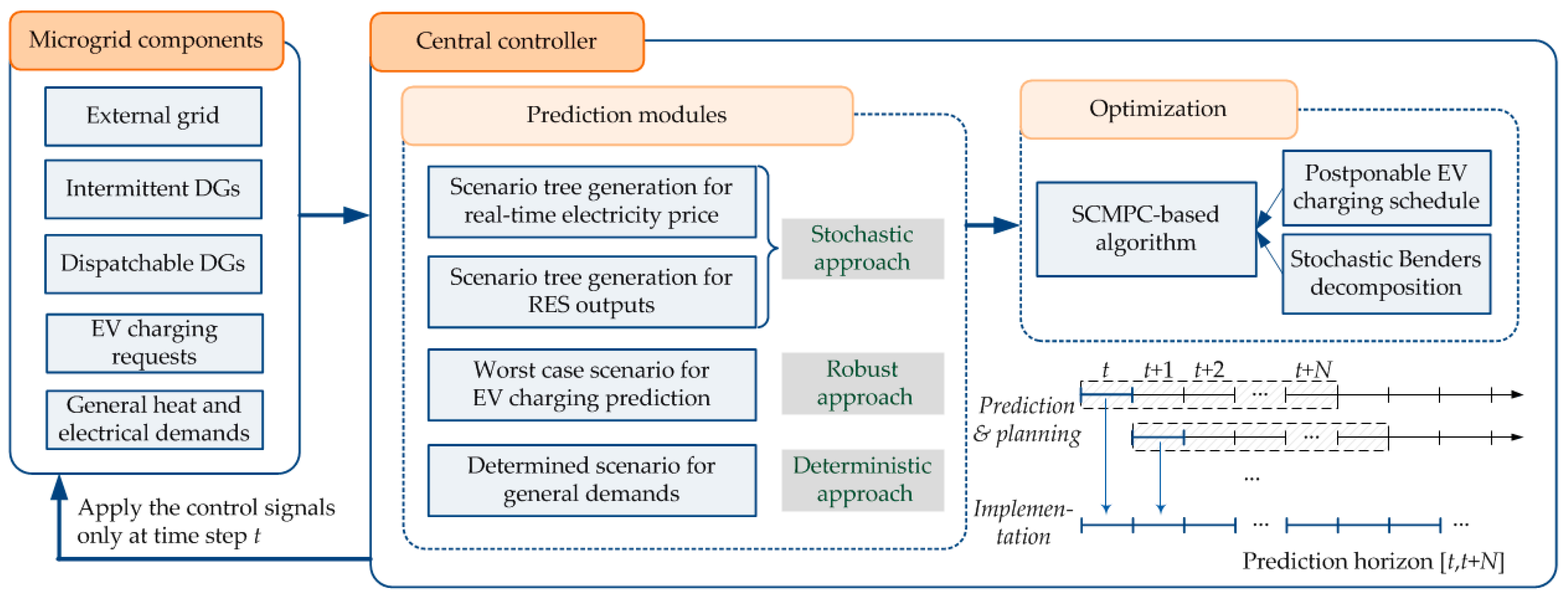
3. A Hybrid Stochastic and Robust MPC Approach for Energy Management

3.1. Structure Model with Operation Constraints

An MPC-based energy management incorporated with uncertainties ξ is formulated to optimize the economic performance with the objective of minimizing the expected sum of the fuel purchasing cost Cf, the electricity purchasing cost from the external grid Cex, and penalties P, such as the self-discharge and wear losses for ESSs or start-up costs for CHPs during the prediction horizon [t,t+N]. At every time step t, the following problem is solved:
inf E [ k = 0 N ( C f , t + k | t + C e x , t + k | t + P t + k | t ) | ξ t + k | t ]
where the symbol Ut+k|t stands for the variable U at time step t + k predicted at time step k. The forecasted uncertainties can be correlated over time; thus, the variable Ut+k|t need not be the same as that of Ut+k+1|t+1. The production costs of RESs (i.e., wind and solar energy) are assumed to be negligible.
Although uncertainties are best modeled as continuous variables for presenting an ideal precise prediction as in Equation (1), integrals are always turned into probability sums based on a finite set of scenarios for the purpose of decreasing high computational complexity based on common sense.

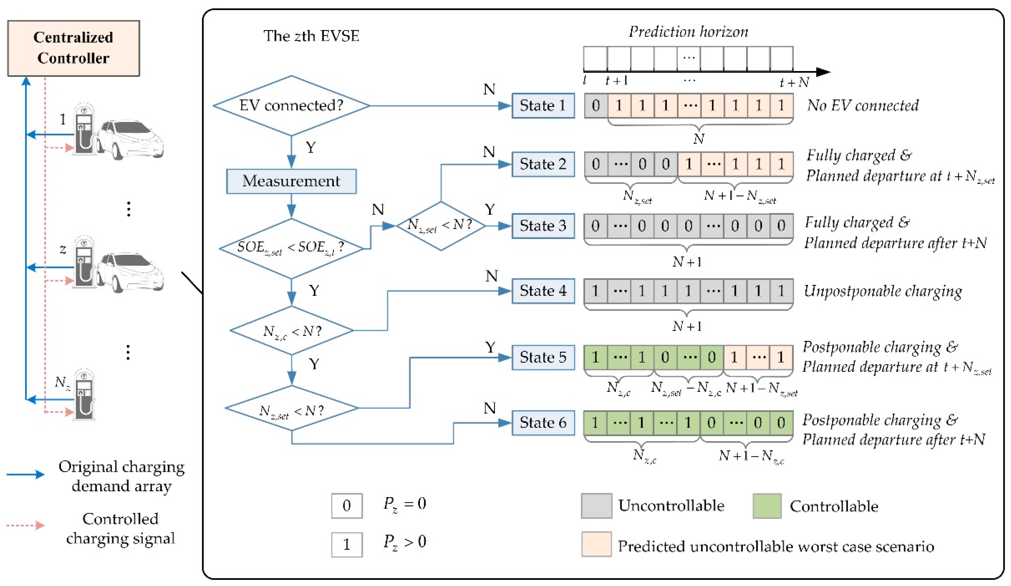
3.2. Robust Approach for EV Charging with Demand-Side Management

3.2.1. Robust Approach for EV Charging Uncertainties

Current approaches specifying EV fleet characteristics neglect the feature that the EV user base is relatively small and of a fast dynamic process since we are still undergoing the early stage of EV diffusion progress. These commonly used parametric distribution characteristics of EV fleets may vary significantly in different microgrids, both at temporal and spatial scales. To overcome the statistical insignificance of EV charging prediction at the current stage of development, a novel robust approach is developed to address EV charging uncertainties for energy management.
Full awareness of prediction information is required for MPC-based energy management in the prediction horizon. For those unknown charging requests, a worst-case scenario is applied by setting a boundary of maximum possible charging loads, where all EVSEs with no EV connection at time step t + k will be plugged in a virtual EV in the following time step t + k + 1. The virtual EV will stay connected to this EVSE until t + N with a requested total charging time that is equal to N − (k + 1). The other worst-case scenario adopted is to deal with uncertainties beyond the prediction horizon for the actually-connected EVs. Despite the fact that the charging loads may be postponable for EVSEs in State 4, since the prediction horizon is less than the parking duration remaining, the charging requests are still treated as unpostponable in the whole [t,t+N]. These two types of worst-case scenario serve as extreme predictions to enhance the robustness.
Despite focusing on the changing numbers of EVs, we turn our attention to the settled EVSEs in a microgrid, with a total number of Nz which remains the same in the prediction horizon. Assume that all of the EVs connected in the microgrid accept DSM as postponable electrical loads. EV owners set up their desired state of energy SOEz,set with an estimated departure time Tz,set when plugging the EV into the zth EVSE. Additionally, a charging behavior binary variable xz,t+k|t is defined to represent whether there is a charging load of the zth EVSE at time step t + k predicted at current time step t.
At each time step t, every EVSE measures its EV connection state and parameters automatically. A state criterion with six possible states of the charging process can be generated in the prediction horizon [t,t+N] as shown in Figure 2. Notice that the charging behavior binary labeled in Figure 2 is arranged by the original order before DSM. To begin with, an EVSE detects whether there is an EV connected. If not, this EVSE is regarded to be in State 1. When there is a connected EV, measure the current state of energy SOEz,t, the charging power Pz, and fetch the value of SOEz,set and Tz,set. Since time is separated into discrete Δt, Tz,set sometimes need to get rounded to an integer by executing Nz,set = ceil(Tz,set/Δt). If the desired SOEz,set is achieved, which means the connected EV is fully charged, compare whether the planned departure time step Nz,set precedes the prediction horizon N or not, where State 2 represents that the EV is going to leave the connected EVSE within the prediction horizon, and State 3 otherwise. If SOEz,set has not been achieved, the difference of SOEz,set and SOEz,t denotes the needed sum of charging time step Nz,c before the EV departures as:
T z , c = S O E z , s e t S O E z , t P z = Δ S O E z P z N z , c = c e i l ( T z , c / Δ t )
If Nz,c is greater than or equal to N, label the EVSE as in State 4. If not, compare the departure time Nz,set and N again; define that an EVSE with Nz,set less than N is in State 5, and otherwise is in State 6.
At the end of this procedure, all EVSEs are able to send their respective states as well as the original charging behavior arrays containing actual demand and worst-case scenarios.

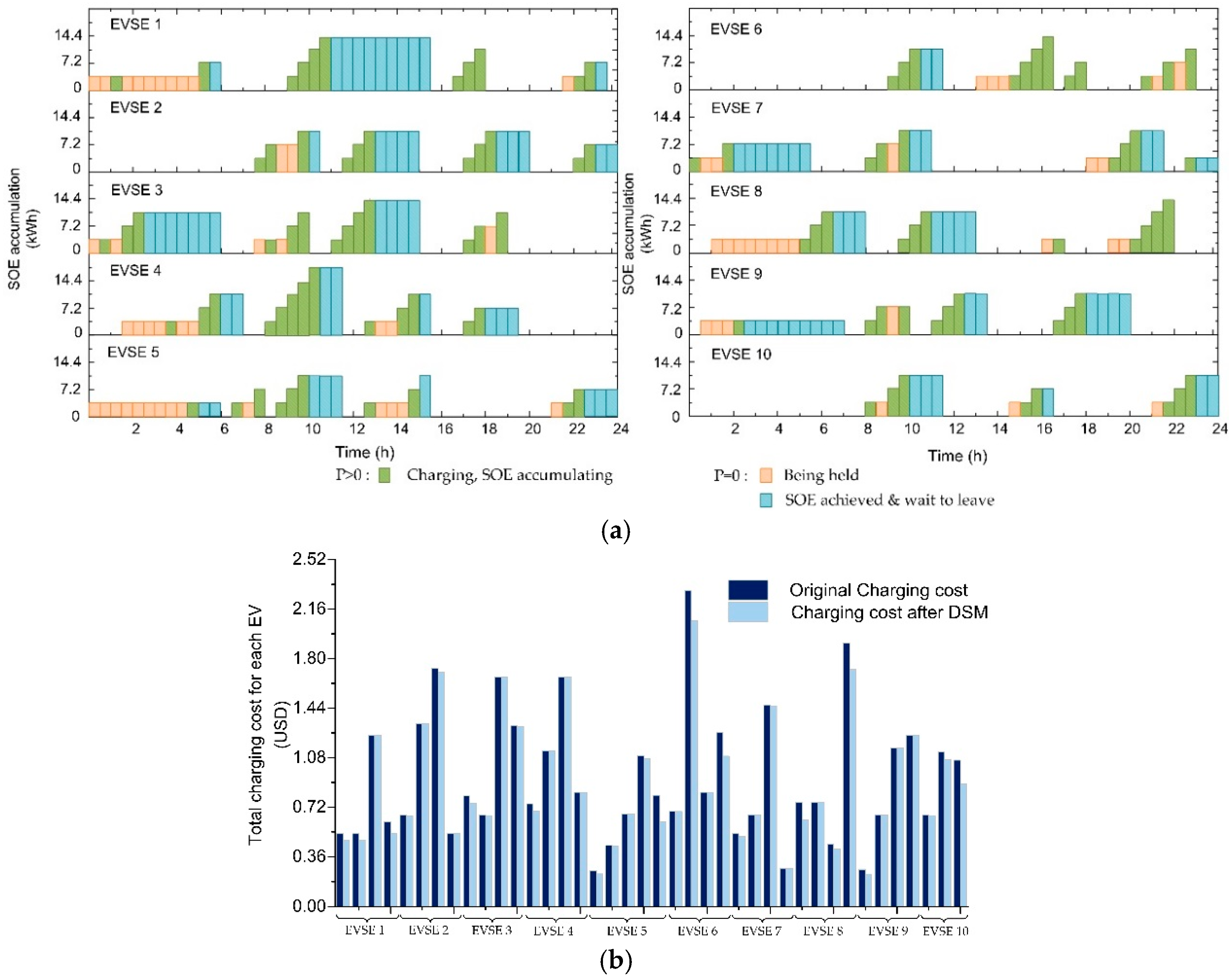
3.2.2. Demand-Side Management for EV Charging

To determine the role of each EVSE in the DSM, the six states are further divided into two groups:
1. Unpostponable group: including State 1, State 2, State 3, and State 4, with a total number of Nz1. The charging loads in the four states are unpostponable within the prediction horizon.
2. Postponable group: including State 5 and State 6, with a total number of Nz2. The charging loads in the two states are postponable without affecting the realization of original charging demand at the end of the prediction horizon. In other words, one or more xz,t+k|t in these states can be scheduled from 1 to 0 or from 0 to 1 without violating the total incremental charging energy needed in [t,t+N]. The scheduled charging behavior Ez,t+k|t should satisfy the following constraints:
t = t t + N E z , D S M , t = N c , z E z    z N z 2 E z , D S M , t { 0 , E z }
Table 1 summarizes all possible circumstances of the charging behavior binary variable xz,t+k|t due to DSM. When there is no charging behavior at time step t + k of the zth EVSE, such as when the desired SOEz,set has been achieved of the actual-connected EV or the charging load is scheduled to be held by the schedule of the energy management with DSM, the value of xz,t+k|t is attributed to be 0; when there is an unpostponable or arranged charging load, then xz,t+k|t is attributed to be 1. In particular, for those EVSEs with virtual-connected EVs, i.e., xz,t+1|t to xz,t+N|t of EVSEs in State 1, and xz,t+k+1|t to xz,t+N|t of EVSEs in State 2 and 5, the charging demands are considered to be unpostponable; thus, the values of these variables above are also assigned to be 1.
Due to the receding horizon philosophy of MPC, all of the arranged EV charging postponements only apply to the current time step t, and the state criterion will be refreshed in the next time step. This allows the update of remotely setting changes of SOEz,set and Tz,set from mobile phones by EV users and hypothetical worst-case scenarios by the system itself. In this way, EMS can achieve a minimized worst-case scenario cost while satisfying charging requirement of every EV user.

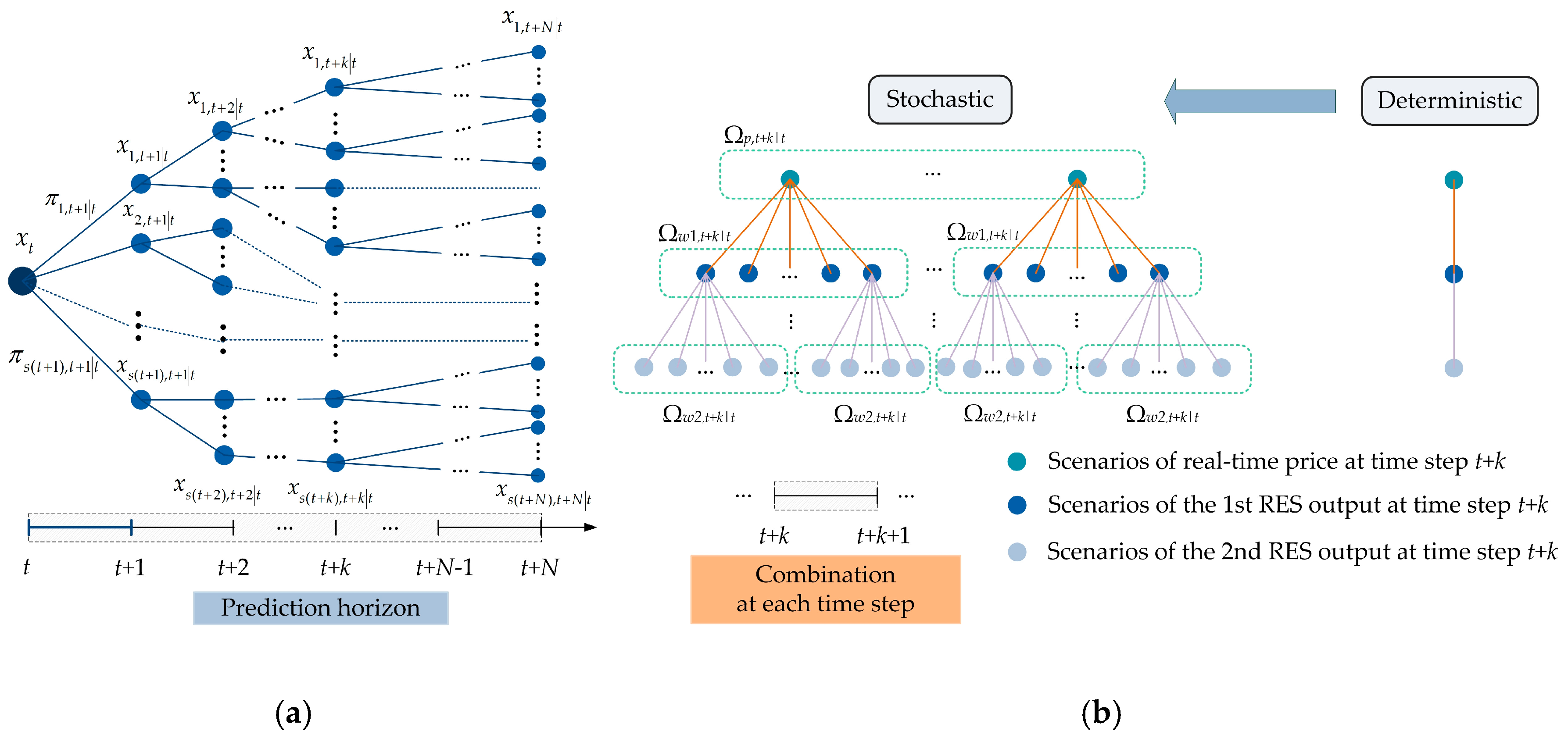
3.3. Stochastic Approach for Uncontrollable Inputs

For uncertainties with relatively accurate prediction models, stochastic approaches allow for the closer imitation of predictions. The so-called scenario tree method has been successfully applied to stochastic models, such as real-time electricity prices, outputs of WTGs, and other RESs. A scenario tree representing uncertainties with a tree of discrete scenarios is shown in Figure 3a with a general structure. In a scenario tree, each node represents a possible state at its particular time step and has only one predecessor, but multiple successors. The root node represents the initial state, and a forward branch from the root node to a leaf node describes a probability-weighted realization. The probability can be even or not, providing a causal but compact representation of the uncertainties acting on the system. A discrete-time formulation for a scenario tree can be written as:
x s ( t + k ) , t + k | t = f ( x p ( t + k 1 ) , t + k 1 | t , u s ( t + k 1 ) , t + k 1 | t , d r ( t + k 1 ) , t + k 1 | t ) π s ( t + k ) , t + k | t = 1 k = 1 , 2 , ... , N 1
where s(t + k) is the total scenario number at time step t + k when predicting at the current time step, and each state xs(t+k),t+k|t is forecasted conditionally on the paths of the preceding time steps, depending on the parent state xp(t+k-1),t+k-1|t, the corresponding control input us(t+k-1),t+k-1|t, and the corresponding disturbance dr(t+k-1),t+k-1|t; and the scenario set is denoted by Ωt+k|t with the sum of the probabilities of πs(t+k),t+k|t at each state being 1. Note that this paper focuses on representing scenarios of forecast uncertainties without the intention to develop or compare their prediction models.
Multiple stochastic uncertainties are considered in this paper, and thus a scenario combination should be considered further. As shown in Figure 3b, a scenario set Ωp,t+k|t of the real-time electricity price pt+k|t, with probabilities of πp,t+k|t and scenario sets Ωwi,t+k|t of the ith RES output Ewi,t+k|t of πwi,t+k|t (i = 1, 2), with the same prediction horizon N, are used to illustrate the scenario combination process at time step t + k. The combination happens at every time step, and each combined scenario consists of the value of a real-time electricity price and RES outputs with a multiplication of their respective probabilities. However, it is noticed that even with a properly reduced number of scenarios, the process of combination still brings about an exponential growth in the total scenario number compared to deterministic approaches, which is related not only to the scenario numbers of every stochastic uncertainty adopted, but also to the length of the prediction horizon. To deal with the computing space requirement and computing time beyond practicality, a parallel computing technique incorporated with the objective function will be introduced in Section 4.3.

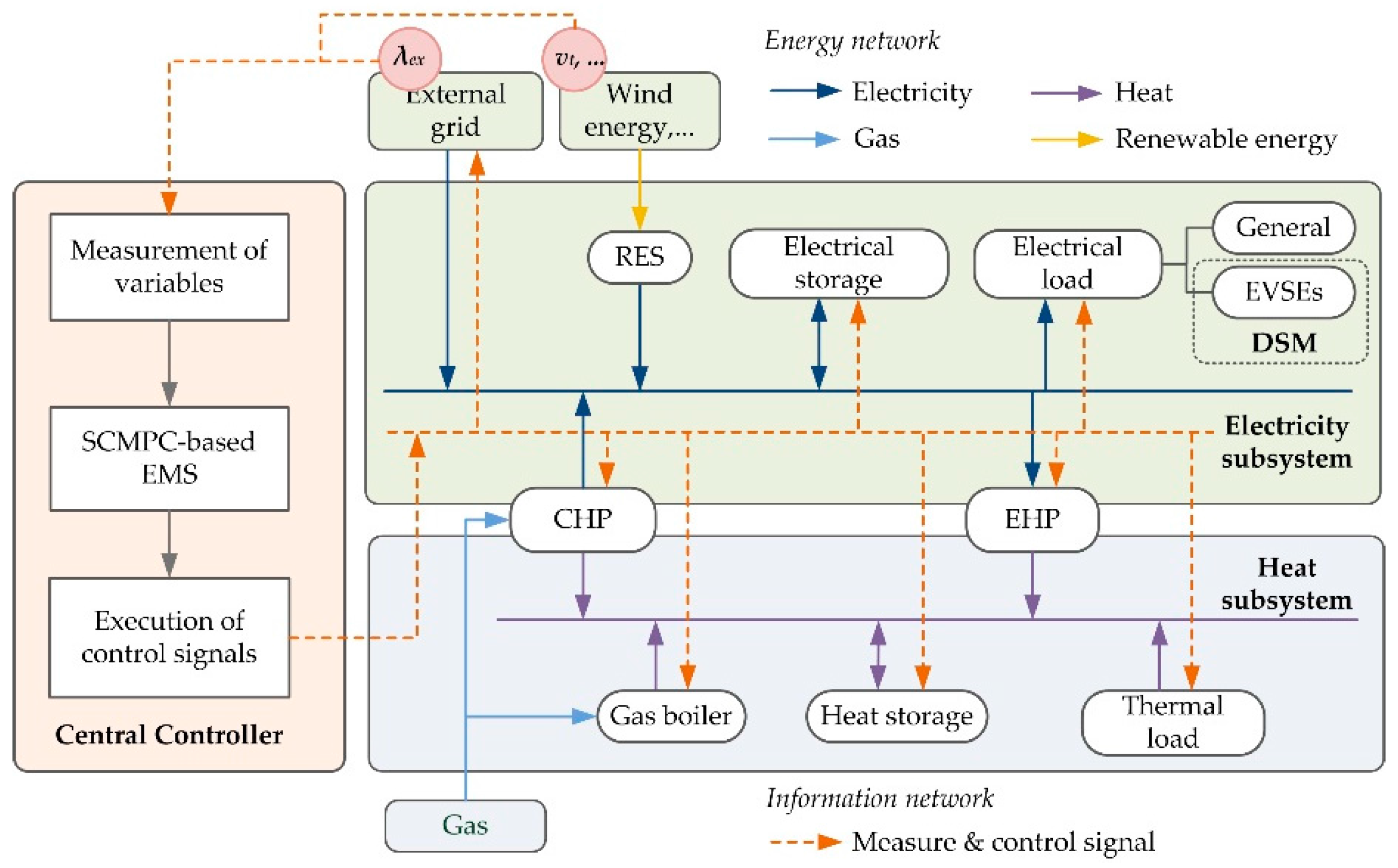
4. Model Formulation for a Combined Heat and Power Microgrid

4.1. Combined Heat and Power Microgrid Model Description

A model of a combined heat and power microgrid is presented for case study purposes, with the basic structure with multi-energy flows depicted in Figure 4. For simplicity, the same type of units are represented as one module here.
The operation constraints of these DG units are introduced as follows:
Taking the wind turbine generator (WTG) as the RES modeled here, its output Ew,t is related with the cut-in speed vin, rated speed vr, and cut-off speed vout. Suppose that it is fully used with no wind curtailment in the microgrid:
E w , t = { 0 0 v t v i n , v t > v o u t P w Δ t ( v t v i n ) / ( v r v i n ) v i n < v t v r P w Δ t v r < v t v o u t
The gas input of a CHP unit Gg,t has a restricted minimum and maximum capacity, Gg,min and Gg,max, respectively. The outputs of electricity production part Eg,t and heat production part Hg,t are constrained by its electrical efficiency ηge,t and thermal efficiency ηgh,t [28]. In a partial load operation, ηge,t may drop approximately linearly by 5%–7% at a minimal part load of 50%, which is considered to be the lower bound Gg,min here, while the total efficiency ηg can be assumed to remain constant:
G g , t = H g , t / η g h , t = E g , t / η g e , t = H g , t η g e , t / ( η g η g e , t ) G g , m i n = 50 % G g , m a x G g , t G g , m a x
The electrical heat pump (EHP) unit is modeled as the air-water type with minimum and maximum thermal capacity Hh,min and Hh,max, respectively. The relationship between heat production Hh,t and electricity consumption Eh,t of an EHP unit is restrained by the coefficient of performance COPh, which can be seen as constant during the analysis horizon:
E h , t = H h , t / C O P h H h , m i n H h , t H h , m a x
Boilers with a coefficient of performance COPl are used as supplementary heat sources because of the wide selectable range of capacity Hl,max complementary to primary heat sources (CHPs and EHPs), with the flexibility of starting up/shutting down quickly. The heat production Hl,t follows:
H l , t = G l , t η l ,       0 H l , t H l , m a x
The battery energy storage system (BESS) is used as the electricity storage here. There are recommended lower and upper limits for the stored energy SOEb,t of the BESS of SOEb,min and SOEb,max, respectively, to extend the battery’s lifetime. Coefficient ηb features the internal self-discharge loss during the last time period [t−1,t]. Coefficients ηb,c and ηb,d feature the charging and discharging efficiency, respectively, with the charging energy donated by Ec,t with a peak value of Ec,max and the discharging energy by Ed,t with Ed,max. SOEb,t is related to Ec,t and Ed,t by:
S O E b , m i n S O E b , t = S O E b , t 1 η b + E c , t η b , c E d , t / η b , d S O E b , m a x 0 E c , t E c , m a x ,     0 E d , t E d , m a x
A water tank is adopted as the heat storage here with an energy capacity Cs. There is an upper limit Hb,max for the imported heat storage Hc,t and exported heat storage Hd,t. Coefficients ηs, ηs,c, and ηs,d are the converted storage, imported, and exported efficiencies, respectively. The heat storage—related behavior and limits are described as:
0 H s , t = H s , t 1 η s + H s , c , t η s , c H s , d , t / η s , d C s 0 H c , t H c , m a x ,   0 H d , t H d , m a x
Electricity demand is divided into two parts: (a) general electricity demand Ee,t; and (b) EV charging demand Eev,t, respectively. The supply side of the electricity subsystem covers the RES output, CHP-produced electricity, scheduled ESS discharging, and purchased electricity from the external grid Eex,t. These supplements cover the total electricity demand, as well as the scheduled ESS charging energy and EHP-consumed electricity. Similarly, the supply side of the heat subsystem, including the heat production of the CHP, EHP, boiler, and scheduled thermal storage charging, should meet with the heat demand Hq,t and discharging of the thermal storage. The co-generation and re-allocation between electricity and heat flows, such as CHPs and EHPs, bring about an interaction in both power flows. The equilibrium of production and consumption in the two energy subsystems must be satisfied simultaneously at every time step t:
E w , t + E g , t + E e x , t + E d , t = E e , t + E e v , t + E h , t + E c , t H g , t + H h , t + H l , t + H d , t = H q , t + H c , t
Note that time is separated into discrete periods by constant time step Δt, and all variables are considered constant within every Δt. The following assumptions are also applied during the formulation of the objective function:
  • The microgrid is generally a price-taker in the market since the upper size of a microgrid is generally limited to a few mega volt-amperes (MVAs);
  • The optimization is based on economic performance, and the general assumption is that voltage and frequency stability control are not considered on this level;
  • The connection between the microgrid and external grid is unconstrained, and thus the output of the installed DGs can be fully absorbed to increase the revenue of the microgrid;
  • Signal delays and transmission losses are not considered.
This model structure can also be expanded to include other DGs, such as photo-thermal (PT) units, combined cooling heating and power (CCHP) units, electrical heater units, etc.

4.2. Implementation of the Energy Management Objective Function

The general objective function in Section 3 minimizing the total operational cost is transformed into a two-stage stochastic programming framework here, and implemented to the microgrid model above. A symbol V t + k | t p , r stands for the corresponding variable V at the pth scenario of the predicted real-time electricity price λ e x , t + k | t p and the rth scenario of the predicted wind power E w , t + k | t r at time step t + k predicted at time step k. The first stage denotes the optimized working state and the gas consumption of the CHP based on the expectation of all scenarios including purchased energies from the external grid, charging schedules for postponable EVs, as well as the scheduling control of EHPs, boilers, and ESSs within their constraints in the second stage. The energy management process is formulated as:
min k = 0 N [ λ f G g , t + k | t X g , t + k | t + F ( X g , t + k | t , X g , t + k + 1 | t ) + p Ω p π p , t + k | t w Ω w π w , t + k | t ( λ e x , t + k | t p E e x , t + k | t p , r + λ f G l , t + k | t p , r ) ] Subject   to : ( a )   Energy   flow   balance E w , t + k | t r + η g e , t + k | t G g , t + k | t X g , t + k | t + E e x , t + k | t p , r + E d , t + k | t p , r = E e , t + k | t + z = 1 N z 1 E z , t + k | t + z = 1 N z 2 E z , D S M , t + k | t p , r + E h , t + k | t p , r + E c , t + k | t p , r η g h , t + k | t G g , t + k | t X g , t + k | t + H h , t + k | t p , r + H l , t + k | t p , r + H d , t + k | t p , r = H q , t + k | t + H c , t + k | t p , r ( b )   DSM   of   postponable   EV   charging   requests t = t t + N E z , D S M , t p , r = N c , z E z z N z 2 , E z , D S M , t p , r { 0 , E z } ( c )   Operational   contraints   of   components S O E b , m i n S O E b , t + k | t p , r = S O E b , t + k 1 | t η b + E c , t + k | t p , r η b , c E d , t + k | t p , r / η b , d S O E b , m a x 0 E c , t + k | t p , r E c , m a x ,   0 E d , t + k | t p , r E d , m a x 0 H s , t + k | t p , r = H s , t + k 1 | t η s + H c , t + k | t p , r η s , c H d , t + k | t p , r / η s , d C s 0 H c , t + k | t p , r H c , m a x , 0 H d , t + k | t p , r H d , m a x E h , t + k | t p , r = H h , t + k | t p , r / C O P h , H h , m i n H h , t + k | t p , r H h , m a x H l , t + k | t p , r = G l , t + k | t p , r η l , 0 H l , t + k | t p , r H l , m a x
where the fuel price λf, as the natural gas price here, is seen as a constant in the predicted horizon; the binary variable Xg,t+k|t is given as 1 to denote that the CHP unit is on at time t + k predicted at time k, and 0 otherwise; and a penalty function F(Xg,t+k-1|t, Xg,t+k|t) is used to restrict frequent changes of the on/off working state, reflecting the nontrivial start-up and shut-down cost of the CHP.
Given the nature that CHPs should not change their on/off states too frequently, the variables to be scheduled in the first stage pertain to the CHP unit that interacts with the scenarios of all the stochastic processes instead of being explicitly linked to one specific scenario. Such a structure not only reduces the computing space and variables by separating the working binary state, but is also perfectly suitable for incorporating with the BD technique.

4.3. Benders Decomposition

As discussed in Section 2.1, the Benders decomposition is one of the most widely used decomposition methods with proven efficacy. It improves the convergence time by separating the original optimization problem into a two-fold structure: a master problem for optimizing the first-stage problem bounded by the Benders cut, and a sub-problem which is impacted by the trial solution from the master problem. When applied to stochastic problems, the BD performs parallel computing on solving a set of sub-problems as smaller deterministic-equivalent problems simultaneously, which reduces the computational burden and accelerates the convergence time [29].
The master problem determines the trial solution for the first-stage decisions subjected to the approximate solutions of the sub-problems as a set of constraints added on each iteration, namely the Benders cuts. In this particular case, the first-stage decisions are the binary variable of the CHP working state in [t,t+N]:
Z μ = min k = 0 N [ λ f G g , t + k | t X g , t + k | t + F ( X g , t + k 1 | t , X g , t + k | t ) + θ k ] θ μ p Ω p π p , t + k | t w Ω w π w , t + k | t [ Q μ , p , w , t + k | t ε μ , p , w G g , t + k | t ( X μ , g , t + k | t X ¯ μ , g , t + k | t ) ]
where θμ is the Benders cut in iteration μ describing the second-stage value based on the previously-determined first-stage decisions, Qμ,p,w,t+k|t is the value of sub-problems at iteration μ and the pth, ωth scenario, εμ,p,w is the extreme direction or sensitivity for the corresponding Qμ,p,w,t+k|t, Xμ,g,t+k|t is the trial solution determined in iteration μ. In the initial step (μ = 1), optimality cuts are not considered.
The trial solution Xμ,g,t+k|t in iteration μ is passed as an input parameter to sub-problems subject to constraints in Equation (12); then a solution for the second-stage decisions is determined. Each scenario will generate a different sub-problem objective function which shares a similar formulation but different input parameters. The sub-problems minimize the electricity purchase and boiler consumption with the trial CHP working action by:
Q μ , p , w , t + k | t = min ( λ e x , t + k | t p E e x , t + k | t p , r + λ f G l , t + k | t p , r ) s . t .   Equation   ( 12 )   ( a ) ( c )
A convergence criterion is used to stop the algorithm when the gaps between the master problem and sub-problems are within a pre-defined tolerance. While the value of the master problem is set up as a lower bound (LB), the upper bound (UB) of the optimal solution is represented by the trial solutions of the sub-problems. The convergence criterion is formulated as:
LB UB δ LB UB = λ f G μ , g , t + k | t X ¯ μ , g , t + k | t + F ( X ¯ μ , g , t + k 1 | t , X ¯ μ , g , t + k | t ) + p Ω p π p , t + k | t w Ω w π w , t + k | t Q μ , p , w , t + k | t LB = Z μ
where it is assumed that the difference δ between the bounds will be lower than or equal to 0.1%LB.
The solution procedure of the stochastic BD with the receding horizon policy applied to MPC is represented below (see Algorithm 1).
Algorithm 1. Stochastic BD
At each time step t do
Initialize μ = 1, UB = +∞, LB = −∞, θ = 0
For k = 1 to N
Set μ = 0, do
  Solve master problem in Equation (13) and determine a trial solution Xμ,g,t+k|t
  Update the value for LB
  Solve all sub-problems in Equation (14) with trial solution Xμ,g,t+k|t
  Update the value for UB
if LB/UB > δ then
  Add the new optimality cut θ associated with iteration μ to the master problem
  Set μ = μ + 1, and repeat the solution procedure
else
  an optimal solution is achieved, and execute the control signals at time step t
end for

5. Case Study

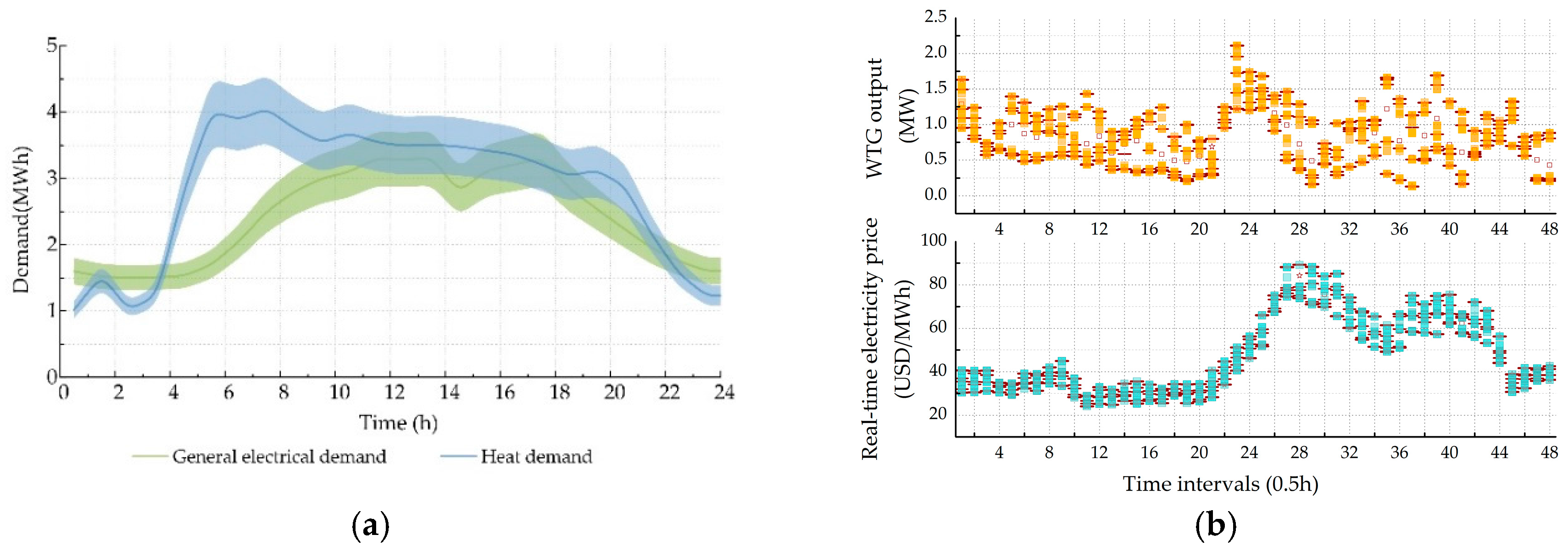
5.1. Numerical Specifications

The proposed approach is applied to a hybrid heat and power microgrid model of campus size with the numerical parameters of the components specified in Table 2.
A total analysis horizon of 24 h is adopted here. The distributions of scenarios with probabilities for the WTG output and the real-time electricity price are shown in Figure 5a. The heat and general electricity demand predictions are treated as a forecast with a standard deviation range εd of 25%, as shown in Figure 5b. The gas price is treated as a constant value of $49.2 USD/MWh.
Ten EVSEs with a same charging power Pz of 7.2 kW are installed in the microgrid. For simplification, the total needed charging energy ΔSOE for each EV is calculated in advance as the difference between a desired SOEz,set and the initial SOE when arriving. To display the EV charging demands intuitively, the actual EV admissions of each EVSE including total charged energy ΔSOE, arrival time Tz,arr, and departure time Tz,set are rounded up and are organized in the form of {ΔSOE, Tz,arrTz,set} where the unit (kWh) is omitted for simplicity. For instance, an array of {7.2, 0:00–6:00} signifies that this EV arrives at 12 a.m. and leaves at 6 a.m. with a total needed charging energy of 7.2 kWh. Every EVSE can be plugged with no more than one EV at the same time. EV charging demands for the simulation are listed in Table 3. Although we regard these as non-perfectly-matched stochastic models for EV charging behavior in microgrids at this stage, the distribution sampled in Table 3 fits some accepted statistical information about travel patterns of vehicle users, such as in [30,31], other than randomized samples.
All numerical simulations are solved in MATLAB on an Intel i3 3.2 GHz Windows-based PC with 4 GB of RAM. The proposed approach is compared with some other approaches on the same model, although detailed outputs may differ significantly due to different settings of a microgrid.

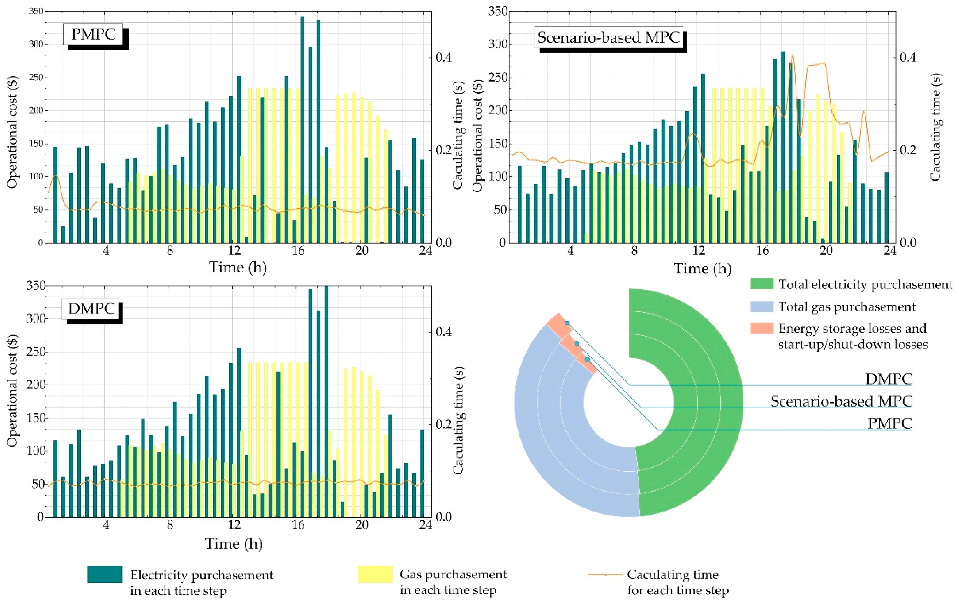
5.2. Simulation and Discussion

5.2.1. Dealing with Robust and Stochastic Uncertainties

In order to exemplify the economic performance of the proposed scenario-based MPC approach, it is compared against DMPC, where these scenarios of stochastic variables are replaced by only one scenario in their predictions, and precise MPC (PMPC), where perfect deterministic foresight on the predicted inputs is assumed. Due to its ideality, PMPC is taken as the benchmark example for forecast accuracy with no uncertainties. For all three MPC-based approaches, the analysis horizon is conducted for each time period interval at 0.5 h, and the prediction horizon N = 16.
Figure 6 shows the results of these three approaches. PMPC with perfect future information attains a prominent behavior of overall expenditure, as expected. The accumulated operating cost for the proposed scenario-based MPC is $10,898.07 USD/day, which is the closest to PMPC, and saves the cost of 0.955% in the analysis horizon compared with DMPC. As to the computing time, no major difference is detected between DMPC and PMPC since both of them equivalently contain only one scenario. However, there is an observable deceleration of the convergence speeds for scenario-based MPC compared with the others due to the involvement of many more scenarios than the traditional one-scenario procedures. It is clear that when prediction uncertainty is inevitable in general, scenario-based MPC outperforms in reducing the total operating cost compared to DMPC at the expense of the computing time.
To further illustrate the DSM process of EV charging, Figure 7 shows the charging behavior schedule with accumulated SOE and the charging cost of each EV. Instead of executing a straightforward strategy as immediate and uncoordinated charging, postponements of EV charging are arranged by energy management to coordinate with the operational cost optimization of the microgrid as shown in Figure 7a. It can be seen in Figure 7b that each EV copes with a flat or declining charging cost after DSM, where the EV owners can also benefit from participating in the energy management. Since the objective function focuses on minimizing the total operational costs, the postponements often occur in the time steps with higher electricity prices or with lower local energy outputs in the prediction horizon, resulting in the reduced charging expenditure for each EV. The DSM cannot be achieved without the worst-case scenario for the unknown charging demand prediction while the robustness of the worst-case scenario ensures that the requested EV charging demand is fulfilled when an EV is leaving.
Figure 8 is supplemented to show the supply-demand balance of the electrical and heat flow by scenario-based MPC. Useful future information may affect the current decision more accurately at each time step, and the expected optimization can be scheduled more precisely by taking account of stochastic scenarios in advance, i.e., before peaks of the real-time electricity price and the demands.

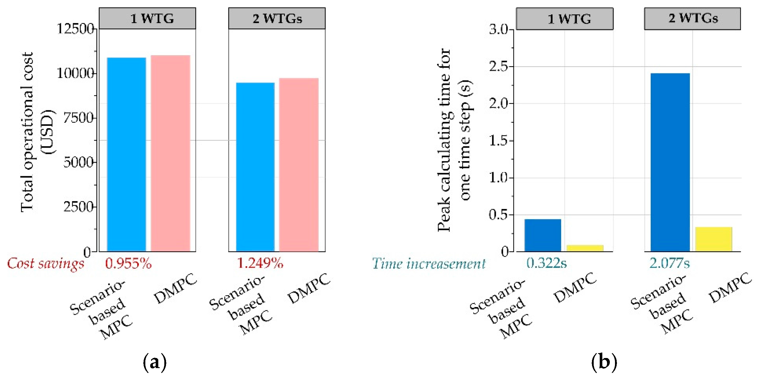
5.2.2. Dealing with Increasing Scenario Sizes

As concluded, the proposed scenario-based MPC approach gains a lower operational cost but consumes more computing time. With the trend of progressive RES penetrations, this study case is simulated to investigate the importance of considering the computing performance while maintaining a good economic performance of scenario-based MPC. Assume that two WTGs with the same parameters are installed in the microgrid above, sharing dissimilar meteorological environments which lead to diverse wind speed scenarios. Figure 9 depicts the total operational cost and the peak calculating time for one time step in the whole simulated analysis horizon (N = 16). When uncertainties in the microgrid increase, the gap of the total operational cost between scenario-based MPC and DMPC also increases; in this particular case study, the cost savings rises from 0.955% to 1.249%. However, there is a significant drawback of the computing time observed, where the peak calculating time increase rises from 0.322 s to 2.077 s. A similar situation happens if more units of RES are integrated, since the problem dimension increases inevitably on account of more scenarios in the scenario combination.
The results of scenario-based MPC with BD are shown in Table 4 to verify whether efficient solutions can achieved in a reasonable computational time. As expected, with the help of BD, the computing times of scenario-based MPC accelerate significantly, and the gap of the computing times between them is acceptable, which makes the proposed approach quite competitive. Meanwhile, the total operational cost is quite similar to that of the original scenario-based MPC approach without parallel computing. By using BD, energy management is capable of providing optimized solutions provided scenario-based MPC while ensuring a competitive computing performance with DMPC.
In addition to the scalability of integrated RES, different prediction models with various scenario generation and reduction methods can also result in increased combined scenario numbers, which lead to high volumes of variables. The adoption of BD makes the energy management systems able to choose applicable prediction models and suitable prediction horizons with more flexibility.

6. Conclusions

This paper presents a scenario-based MPC approach which enables the energy management system of a microgrid to improve the economic performance considering various characteristics of uncertainties. As for uncertainties of a robust nature, here, the EV charging loads at the present stage, a worst-case scenario, as well as the DSM are presented coping with the receding prediction horizon; as for the uncertainties of a stochastic nature, such as RES outputs and the real-time electricity price, the probabilistic scenarios are introduced while the computational efficiency of the objective function is improved by applying the BD technique. The numerical simulations indicate that the proposed approach offers cumulative cost savings while satisfying consumers' demands under a computationally tractable process. Moreover, the proposed approach can be tailored to microgrid applications with more DGs due to the scalability and flexibility to promote full-scale commercial microgrids. Future work could also be extended by incorporating the approach with available EV charging load prediction models when the penetration rate of EVs in a microgrid is adequate enough.

Acknowledgments

This work was supported by the National Key Research Program of China (No. 2016YFB0101800), the National Nature Science Youth Foundation of China (No. 51507032), the Science and Technology Support Program of Jiangsu Province (No. BE2014023), and the Project of State Grid Corporation of China (SGTYHT/14-JS-188).

Author Contributions

Zhenya Ji, Xueliang Huang and Houtao Sun conceived and designed the experiments; Houtao Sun performed the experiments; Zhenya Ji and Xueliang Huang analyzed the data; Changfu Xu contributed practical experiment data and performed simulation verification; Zhenya Ji wrote the paper; Xueliang Huang revised and approved the manuscript.

Conflicts of Interest

The authors declare no conflict of interest.

References

  1. Khodaei, A.; Shay, B.; Mohammad, S. Microgrid planning under uncertainty. IEEE Trans. Power Syst. 2015, 30, 2417–2425. [Google Scholar] [CrossRef]
  2. Song, N.; Lee, J.; Kim, H. Optimal electric and heat energy management of multi-microgrids with sequentially-coordinated operations. Energies 2016, 9. [Google Scholar] [CrossRef]
  3. Ahmad, K.; Naeem, M.; Iqbal, M.; Qaisar, S.; Anpalagan, A. A compendium of optimization objectives, constraints, tools and algorithms for energy management in microgrids. Renew. Sust. Energ. Rev. 2016, 58, 1664–1683. [Google Scholar] [CrossRef]
  4. Lin, W.; Tu, C.; Tsai, M. Energy Management Strategy for Microgrids by Using Enhanced Bee Colony Optimization. Energies 2015, 9, 5–20. [Google Scholar] [CrossRef]
  5. Liang, H.; Zhuang, W. Stochastic modeling and optimization in a microgrid: A survey. Energies 2014, 7, 2027–2050. [Google Scholar] [CrossRef]
  6. Shariatzadeh, F.; Mandal, P.; Srivastava, A. Demand response for sustainable energy systems: A review, application and implementation strategy. Renew. Sust. Energy Rev. 2015, 45, 343–350. [Google Scholar] [CrossRef]
  7. Hu, J.; Morais, H.; Sousa, T.; Lind, M. Electric vehicle fleet management in smart grids: A review of services, optimization and control aspects. Renew. Sust. Energy Rev. 2016, 56, 1207–1226. [Google Scholar] [CrossRef] [Green Version]
  8. Parisio, A.; Rikos, E.; Glielmo, L. A model predictive control approach to microgrid operation optimization. IEEE Trans. Syst. Technol. 2014, 22, 1813–1827. [Google Scholar] [CrossRef]
  9. Hussain, A.; Bui, V.; Kim, H. Robust optimization-based scheduling of multi-microgrids considering uncertainties. Energies 2016, 9. [Google Scholar] [CrossRef]
  10. Zheng, Q.; Wang, J.; Liu, A. Stochastic optimization for unit commitment—A review. IEEE Trans. Power Syst. 2015, 30, 1913–1924. [Google Scholar] [CrossRef]
  11. Schildbach, G.; Fagiano, L.; Frei, C.; Morari, M. The scenario approach for stochastic model predictive control with bounds on closed-loop constraint violations. Automatica 2014, 50, 3009–3018. [Google Scholar] [CrossRef]
  12. Mayne, D. Model predictive control: Recent developments and future promise. Automatica 2014, 50, 2967–2986. [Google Scholar] [CrossRef]
  13. Wang, Z.; Chen, B.; Wang, J.; Kim, J.; Begovic, M. Robust optimization based optimal DG placement in microgrids. IEEE Trans. Smart Grid 2014, 5, 2173–2182. [Google Scholar] [CrossRef]
  14. Kim, S.; Giannakis, G. Scalable and robust demand response with mixed-integer constraints. IEEE Trans. Smart Grid 2013, 4, 2089–2099. [Google Scholar]
  15. Liu, G.; Xu, Y.; Tomsovic, K. Bidding strategy for microgrid in day-ahead market based on hybrid stochastic/robust optimization. IEEE Trans. Smart Grid 2016, 7, 227–237. [Google Scholar] [CrossRef]
  16. Gerards, M.; Hurink, J. Robust peak-shaving for a neighborhood with electric vehicles. Energies 2016, 9. [Google Scholar] [CrossRef]
  17. Kou, P.; Liang, D.; Gao, L.; Gao, F. Stochastic coordination of plug-in electric vehicles and wind turbines in microgrid: A model predictive control approach. IEEE Trans. Smart Grid 2016, 7, 1537–1551. [Google Scholar] [CrossRef]
  18. Aziz, M.; Oda, T.; Mitani, T.; Watanabe, Y.; Kashiwagi, T. Utilization of Electric Vehicles and Their Used Batteries for Peak-Load Shifting. Energies 2015, 8, 3720–3738. [Google Scholar] [CrossRef]
  19. Soman, S.; Zareipour, H.; Malik, O.; Mandal, P. A review of wind power and wind speed forecasting methods with different time horizons. In Proceedings of North American Power Symposium, Arlington, VA, USA, 26–28 September 2010; pp. 1–8.
  20. Haque, A.; Nehrir, H.; Mandal, P. A hybrid intelligent model for deterministic and quantile regression approach for probabilistic wind power forecasting. IEEE Trans. Power Syst. 2014, 29, 1663–1672. [Google Scholar] [CrossRef]
  21. Bello, A.; Reneses, J.; Muñoz, A.; Delgadillo, A. Probabilistic forecasting of hourly electricity prices in the medium-term using spatial interpolation techniques. Int. J. Forecast. 2016, 32, 966–980. [Google Scholar] [CrossRef]
  22. Li, Z.; Zang, C.; Zeng, P.; Yu, H. Combined two-stage stochastic programming and receding horizon control strategy for microgrid energy management considering uncertainty. Energies 2016, 9. [Google Scholar] [CrossRef]
  23. Zakariazadeh, A.; Jadid, S.; Siano, P. Economic-environmental energy and reserve scheduling of smart distribution systems: A multi-objective mathematical programming approach. Energy Convers. Manag. 2014, 78, 151–164. [Google Scholar] [CrossRef]
  24. Gröwe-Kuska, N.; Heitsch, H.; Romisch, W. Scenario reduction and scenario tree construction for power management problems. In Proceedings of the Power Tech Conference, Bologna, Italy, 23–26 June 2003.
  25. Feng, Y.; Ryan, S. Scenario construction and reduction applied to stochastic power generation expansion planning. Comput. Oper. Res. 2013, 40, 9–23. [Google Scholar] [CrossRef]
  26. Pereira, M.V.; Pinto, L.M. Multi-stage stochastic optimization applied to energy planning. Math. Program. 1991, 52, 359–375. [Google Scholar] [CrossRef]
  27. Benders, J. Partitioning procedures for solving mixed-variables programming problems. Numer. Math. 1962, 4, 238–252. [Google Scholar] [CrossRef]
  28. Harb, H.; Reinhardt, J.; Streblow, R.; Müller, D. MIP approach for designing heating systems in residential buildings and neighbourhoods. J. Bldg. Perform. Simul. 2015, 9, 316–330. [Google Scholar] [CrossRef]
  29. Moreira, R. Business models for energy storage systems. Ph.D. Thesis, Imperial Collage London, London, UK, 2015. [Google Scholar]
  30. Sundstrom, O.; Binding, C. Flexible charging optimization for electric vehicles considering distribution grid constraints. IEEE Trans. Smart Grid 2012, 3, 26–37. [Google Scholar] [CrossRef]
  31. Kim, J.; Kim, S.; Jin, Y.; Park, J.; Yoon, Y. Optimal coordinated management of a plug-in electric vehicle charging station under a flexible penalty contract for voltage security. Energies 2016, 9. [Google Scholar] [CrossRef]
Figure 1. Procedure of the proposed energy management scheme.
Energies 09 00973 g001
Figure 2. State criterion for EVSEs at every time step t.
Energies 09 00973 g002
Figure 3. Brief structure of (a) scenario tree generation; and (b) scenario combination.
Energies 09 00973 g003
Figure 4. Brief structure of a combined heat and power microgrid.
Energies 09 00973 g004
Figure 5. Profiles of (a) scenarios of WTG output and real-time electricity price; (b) general electricity demand (without EV) and heat demand.
Energies 09 00973 g005
Figure 6. Comparison of three different MPC-based approaches.
Energies 09 00973 g006
Figure 7. Scheduled EV charging of each EV connected to the installed EVSEs: (a) charging behavior schedule with accumulated SOE; and (b) charging cost.
Energies 09 00973 g007
Figure 8. Illustration of energy supply-demand dynamics by scenario-based MPC: (a) balance of electricity flow; and (b) balance of heat flow.
Energies 09 00973 g008
Figure 9. Comparison of scenario-based MPC and DMPC with WTG penetration increases: (a) total operational cost; and (b) peak calculating time for one time step.
Energies 09 00973 g009
Table 1. The assignment and circumstances of the charging behavior binary xz,t+k|t.
ValueAssignmentCircumstances
0No charging loadThe desired SOEz,set has been achieved;
Original charging behavior is arranged to be held by DSM.
1Positive charging loadUnpostponable charging of actual-connected EVs;
Unpostponable charging of virtual-connected EVs;
Arranged charging behavior by DSM.
Table 2. Parameters of the modeled microgrid components (half hour-based).
TypeRated PowerOther Parameters
CHPGg,max = 2.45 MWηg = 0.75~0.85, ηge = 0.35~0.40
EHPHh,max = 2.5 MWCOPh = 3.0
BoilerHl,max = 2.65 MWηl,t = 0.85
BESSEc,max = 2.4 MW, Ed,max = 2.4 MWηb,c = 0.95, ηb,d = 0.95, ηb = 0.99,
SOEb,max = 4 MWh, SOEb,min = 0.8 MWh
Water tankEc,max = 2 MW, Ed,min = 2 MWηs,c = 0.90, ηb,d = 0.90, ηs = 0.95,
Cs,max = 26 MWh, Cs,min = 12 MWh
Table 3. Actual EV charging energy, arrival, and departure settings.
EVSE No.EV Charging Request Data
1{7.2, 0:00–6:00}, {14.4, 9:00–15:30}, {10.8, 16:00–18:00}, {7.2, 21:30–23:30}
2{10.8, 7:30–10:30}, {10.8, 11:30–15:00}, {14.4, 16:30–20:30}, {7.2, 22:00–24:00}
3{10.8, 0:00–6:00}, {10.8, 7:30–10:00}, {14.4, 11:00–15:00}, {10.8, 17:00–19:00}
4{10.8, 1:30–7:00}, {18.0, 8:00–11:30}, {10.8, 12:30–15:30}, {7.2, 17:00–19:30}
5{3.6, 1:30–6:00}, {7.2, 6:30–8:00}, {10.8, 8:30–11:30}, {7.2, 12:30–15:30},{7.2, 21:00–24:00}
6{10.8, 9:00–11:30}, {14.4, 13:00–16:30}, {7.2, 17:00–18:00}, {10.8, 20:30–23:00}
7{7.2, 0:00–5:30}, {10.8, 8:00–11:00}, {10.8, 18:00–21:30}, {3.6, 22:30–24:00}
8{10.8, 1:00–8:00}, {10.8, 9:30–13:00}, {3.6, 16:00–17:00}, {14.4, 19:00–22:00}
9{3.6, 0:30–7:00}, {10.8, 8:00–10:00}, {10.8, 11:00–13:30}, {10.8, 16:30–20:30}
10{10.8, 8:00–11:30}, {7.2, 14:30–16:30}, {10.8, 21:00–24:00}
Table 4. Performances under different settings.
Setting ValuesTotal 1 Operational Cost (USD)Peak Calculating Time for One Time Step 1 (s)
Installed WTG numberScenario-based MPCDMPCScenario-based MPCDMPC
without BDwith BDwithout BDwith BD
110,898.0710,902.7611,003.120.4040.0950.082
28944.958957.339056.642.3670.3310.290
1 In a simulated analysis horizon of 24 h.

