The Effect of Biogas Production on Farmland Rental Prices: Empirical Evidences from Northern Italy

Abstract

In the last decade, increased environmental awareness has prompted the adoption of incentives for exploiting renewable energy sources. Among these, biogas production has received a certain attention in developed countries. Nonetheless, the subsidies provided have posed the problem of an activity (the production of bioenergy) that engages in direct competition with food and feed production for limited resources, like agricultural land. Even if this competition may be softened by allocating marginal land and/or using dedicated non-agricultural crops, empirical evidence shows that biogas plants have been developed in highly-productive agricultural areas, using increasing amounts of maize silage as feedstock. Thus, studies aimed at measuring the effect of biogas production on agricultural activities are needed in order to avoid this socially undesirable outcome. The paper presents an econometric estimation of the impact of biogas plants on farmland rental values of a Northern Italian rural area. Results show that biogas has a non-linear effect on rental prices, suggesting that incentive schemes specifically accounting for plants’ dimensions and technologies would improve the social sustainability of the bioenergy sector and its coexistence with agricultural activity.

1. Introduction

Increased environmental awareness, both in public opinion and in governments of many countries, has prompted, over the last decades, the adoption of incentives for exploiting renewable energy sources. Among these, the production of energy from agricultural products, such as biomass and biofuels, generally termed as bio-energies, has received a certain attention in developed countries. The subsidies provided to foster such productions have raised concerns for many reasons: for their cost, compared to employment and welfare gains [1], and for the potential competition with traditional allocations of farmland, devoted to food and feed production. The latter aspect, named as the “food, energy and environment trilemma” [2], poses the problem of a further activity (the production of energy) that engages in direct competition with food and feed production for limited resources like water and agricultural land. As the latter is a fixed, non-renewable factor of production, it is plausible that such competition affects primarily on its allocation and, consequently, on food prices. In this context, the subsidization provided for bioenergy has changed the relative convenience among alternative uses of agricultural land, increasing the relative profitability of crops for energy purposes. For this reason, increasing attention has been paid on potential undesirable effects of such financial incentives on existing supply chains [3,4,5,6]. Even if this competition may be softened by allocating marginal land for energy production [7] and/or using dedicated non-agricultural crops [8], its effects have been perceived as increasingly harmful for other agricultural activities in highly productive areas. Potential negative impacts of bioenergy production may be hampered where the same crop can be allocated to feed both bioenergy plants and livestock. This is, for instance the case of biogas production, which, as a consequence of dedicated subsidization policies, has been developed in highly productive agricultural areas, using increasing amounts of maize silage as feedstock [9]. As suggested by Bartoli et al. [10], an energy policy providing incentives for large-sized biogas plants, fed mainly with maize silage, may increase the demand for such crops, increasing its price and, consequently, both feeding costs for livestock farms and land prices. On the other hand, Bartoli et al. [10] show that an incentive structure more favorable for plants fed mainly with livestock manure—small- and medium-sized—may render biogas production more compatible with other agricultural activity. As the impact of biogas activity may be highly pervasive, its impact on agricultural areas has been explored extensively by means of modelling approaches. On the contrary, contributions focusing on its effect on land allocation and land value and rental prices have been quite limited (see Section 2 for details). The aim of this paper is to contribute to the current literature about the impact of biogas production on the rental prices. To do so, we examine a case study in a province of Northern Italy, where the biogas industry has increased sharply as a consequence of dedicated policies. The same province is also one of the most productive for field crops and livestock, and we wanted to measure the extent to which the competition between biogas and agricultural activities have impacted land rental prices.

The rest of the paper is organized as follows: Section 2 is devoted to the literature on determinants of farmland rental price and previous evidence of the effect of biogas on the farmland market; the case study, the data, and the econometric model are presented in Section 3; results are analytically discussed in Section 4 while, in conclusion, some reflection on possible policy implications of the research findings are gathered.

2. The Impact of Bioenergy on the Land Market: Evidence from the Literature Review

As we are interested in estimating the impact of biogas production on farmland rental values, the literature review is focused, on one hand, on all potential determinants of land value and, on the other hand, on the previous studies specifically addressing this issue.

Factors affecting the value of agricultural land have been extensively examined. A recent review by Feichtinger and Salhofer [11], discussing the relationships between farmland value and agricultural payments, classifies the potential determinants of farmland price in internal/agricultural variables and external variables. The first group includes expected income and wealth from agricultural activity and external subsidies. Indeed, all of the authors agree that the first factor affecting the market of farmland is the rationale farmers’ objective of profit maximization. Thus, the willingness to pay for land is directly related to its expected return, which depends on land use capability [12,13]. The significant effect of public support to agriculture on land value is the second scientific cornerstone. In particular, researchers focused on the extent to which payments are capitalized into farmland [14,15,16,17], some of them using spatial econometrics [18].

As the observation and description of the relationship between external variables and farmland value is complicated, it is more difficult to estimate their impact. Nonetheless, Feichtinger and Salhofer [11] describe the three aspects that have been considered and measured by researchers and steadily entered in the literature. They refer to the micro and macroeconomic context and the urban competition for land. Microeconomic variables link to competition for land due to its possible alternative use, such as livestock feeding [19] and manure density [20], controlling for the location and dimension of the market [21]. Some adjustments have also been proposed considering the macroeconomic indices of inflation and interest rate, the taxation costs connected to the farmland market and the availability of bank credit [22]. Obviously the competition for land is especially exerted by non-agricultural activities, whose effect is often controlled using indices of rurality and/or urbanization, such as population density, distance from nearest cities, or relative importance of agriculture in the region [12] and, more recently, by quantification of non-market amenities of the location [23].

Specifically, the impact of bioenergy on farmland use and value has been tackled from different perspectives. Some studies propose an approach based on the observation and description of the phenomenon from a qualitative and/or institutional point of view. An extensive general review collecting findings from reports considering European countries has been proposed by Swinnen et al. [24]. The research suggests that bioenergy is expected to exert an effect on farmland market in Germany, Netherlands, and Sweden. Carrosio [25,26] proposes an institutional interpretation of the biogas context in Italy which discusses different scenario analyses deriving from potential changes in actual European bio-energy policies. Other studies present a modelling approach. For example, Johansson and Azar [27] simulate the effects of a new climate policy scenario in the US supporting biomass per bioenergy productions and calculate that the price of the farmland rental price could increase five times by 2100. Mela and Canali [9] calculate the land required for energy production depending on the substrate, thus suggesting different degrees of competition per different energy policy scenario. Furthermore, papers by Ostermeyer and Schönau [28] and Appel et al. [29] are based on agent-based modeling whose results predict that biogas may be more profitable for larger and more competitive farms at the social cost of increasing the value of land, thus decreasing the market power of smaller farmers. Finally, there are limited contributions that apply econometric methods to measure the effect of biogas on farmland rental price. On the contrary, we are not aware of any research that uses biogas plant characteristics as independent variables, while the following papers enter this information as control parameters of the models. In the research by Kilian et al. [16] an analysis on Bavarian cross-sectional data on land rental prices are presented. The installed kW per hectare at the municipality level explains the increased demand for land for energy crops resulting in positive significance on the utilized agricultural area (UAA) rental price. Emmann et al. [30] present results from a survey conducted on 246 German farmers, estimating that the presence of biogas plants in a 10 km radius has a weak significance over the maximum land rental price, while the installed biogas power seems to have no effect on farmland price. Lastly, Hüttel and Odening [31] used the data from public bids for farmland allocation entering the installed kW per hectare in an agrarian region in the model and finding a positive correlation with rental value.

3. Data and Methods

3.1. The Analytical Framework: The Hedonic Pricing Model

Researchers interested in explaining the impact of different variables on farmland price may normally refer to two different approaches, namely the net present value (NPV) model and the hedonic pricing (HP) model [11]. The two methods propose different frameworks for the analysis of the same issue. The NPV model argues that farmers are willing to pay a maximum price for land that equals the expected returns and costs of using that land in the future. On the other hand, the HP model describes the land as a good composed of different attributes, as proposed by Lancaster [32] and Rosen [33]. Thus, the price that farmers are willing to pay for land is linked to the value/disvalue the farmers recognize as farmland attributes at fixed market conditions. Despite this differentiation, linear regression analysis is normally used to calculate the impact of explanatory variables on farmland price in both models.

We decided to frame the analysis using the HP model, because it is suited to identify the significant shifters to the land price and quantify their impact. The HP model is thus used to approximate R, the farmland rent value, by a set of attributes A following the equation:

$$R=\mathsf{\alpha }+\mathsf{\beta }A+\mathsf{\epsilon }$$

(1)

where α is a constant, $\mathsf{\beta }$ represents the vector of parameters that will be estimated, and $\mathsf{\epsilon }$ is the error term. As suggested by Feichtinger and Salhofer [11] the $A$ attributes that create land value (that reasonably applies also for land rent) can be classified in internal and external agricultural variables. Indicating by $I$ and $E$ these two groups of predictors, Equation (1) becomes:

$$R=\mathsf{\alpha }+\mathsf{\delta }I+\mathsf{\rho }E+\mathsf{\epsilon }$$

(2)

where δ and $\mathsf{\rho }$ are vectors of internal and external agricultural variables respectively. Referring to the shifters of biogas plants to farmland value, called B, they can be considered external agricultural variables; thus, Equation (2) turns into:

$$R=\mathsf{\alpha }+\mathsf{\delta }I+\left(\mathsf{\vartheta }B+\mathsf{\gamma }O\right)+\mathsf{\epsilon }$$

(3)

Equation (3) helps to separate the effect of biogas plants characteristics from other external variable, indicated by O. Given this framework, in order to analyse the effect of biogas plants on land rental prices, we used regression analysis in the form of ordinary least squares (OLS) to estimate the coefficients of Equation (3). Applying the HP principles, the significant estimated parameters of the equation represent the change in rental price due to the change of the explanatory variable considered, ceteris paribus. In fact, focusing on the effect of biogas plants on price, the vector $\mathsf{\vartheta }$ in Equation (3) is interpreted as:

$$\mathsf{\vartheta }=\frac{\mathsf{∆}R}{\mathsf{∆}B}$$

(4)

The vector of coefficients ϑ then represents the changes of R due to one-point changes in variable B (biogas plants characteristics—see Appendix A for an easy explanation).

3.2. Case Study and Data: The Land Rent Contracts in the Province of Cremona

The case study is represented by the biogas plants installed and the agricultural land rented in the Province of Cremona. The area is a part of the Po Valley, located in the Lombardy Region in Northern Italy and covers 1771 km² (7.4% of the Lombardy area). The province had 361,610 inhabitants in 2015 (3.6% of the Lombardy and 0.6% of the Italian population, respectively) with a population density of 204.2 inhabitant per square kilometre. According to the most recent available data, the UAA is about 135,531 ha, of which 17.3% is rented with a density of 3.69 livestock units (LU/ha), above an Italian average of 0.77 LU/ha (Our elaboration on Italian National Institute of Statistics–Istat–Census data, 2010). Thus, the Province of Cremona is a relevant case study for the analysis of the effect of the biogas plants characteristics on land rental price, because of the potential competition for land devoted to food, feed, and fuel production, as underlined by Vaccari et al. [34].

The Province of Cremona represents an interesting case study to analyze the effect of the biogas industry on land rental prices, because it has 154 plants, having a total of 104,947 kW installed up to 2014. The total nominal capacity installed in the area suggests that farmers producing food and feed crops may be subject to an increase of land rental prices due to the growing demand of land for energy crops. Furthermore, given the variability in terms of total and average kW installed within the Province, as shown in Figure 1, it is supposed that the effect on the land rental market can be measured under different conditions, allowing testing whether, and to what extent, the presence of biogas plants influences land rental prices.

In order to study the change in land rental prices due to the presence and characteristics of biogas plants in the Province of Cremona, we used data from different institutional databases. In particular, land rental contract characteristics belong to information owned and gathered by the Associazione fra proprietari di Fondi Rustici della Provincia di Cremona (Association of Landowners Cremona province). This dataset is based on 2063 contracts signed between 2010 and 2014 by landowners and farmers from the Province of Cremona and contains the information on land rental prices and relevant cadastral data, such as the total rented area and the average dimension of rented land units. From the agricultural information system of the Lombardy Region we collected data on tenant characteristics, such as farm economic size (measured in standard output), type of farming, and agricultural use of rented land. Finally, the national databases of the Agricultural and Demographic Census of Istat provided information on agricultural activity at the municipality level (livestock unit, UAA, and dimension of municipalities), while data on biogas plant characteristics (location at the municipality level and nominal capacity, i.e., installed power in kW) have been collected from Gestore Servizi Elettrici (GSE) Spa (http://www.gse.it/en/Pages/default.aspx). Data from different databases have been merged with the lease contracts according to the cadastral information of the rented farmland plots’ and their municipality location.

We entered into the model the value of farmland rentals as the dependent variable, while the independent variables used to explain its variability have been chosen according to the framework proposed by Feichtinger and Salhofer [11] and their availability and adequateness. Particularly, it is worth nothing that soil quality and macroeconomic measures are not considered because they are available at a geographical scale that do not offer sufficient variance within the objects in the sample. For the sake of brevity,

Table 1. Description of dependent and explicatory variables used to describe variability in land rental prices.

Variables	Description of the Variable	Unit of Measure	Explanation of Land Rent Values
			Internal/Agricultural Variables		External Variables
			Returns from Agricultural Production	Government Payments	Variables Describing the Market	Urban Pressure Indicators
Rent value (Dependent)	Price of land rental per hectare per year	€/ha
Biogas plants related variables
pl_m	Number of biogas plants per municipality	Number of plants	X		X
kw_m	Kilowatt per hectare of utilized agricultural area in the municipality	kW/ha	X		X
pp_m	Average power of biogas plants in the municipality	kW	X		X
pl_r	Number of biogas plants per agrarian region	Number of plants	X		X
kw_r	Kilowatt per hectare of utilized agricultural area in the agrarian region	kW/ha	X		X
pp_r	Average power of biogas plants in the agrarian region	kW	X		X
liv	Livestock unit per utilized agricultural area in the municipality	LU/ha	X
Agricultural land use—Reference = w&u_s
w&u_s	Share of land used for wood crops or uncultivated	% (ha/ha)	X
mai_s	Share of land used for maize and/or arable crops	% (ha/ha)	X
ene_s	Share of land used for energy crops	% (ha/ha)	X
foa_s	Share of land used for forage alternation	% (ha/ha)	X
fop_s	Share of land used for permanent forage	% (ha/ha)	X
veg_s	Share of land used for vegetables	% (ha/ha)	X
vif_s	Share of land used for vine and/or orchard	% (ha/ha)	X
nur_s	Share of land used for plant nursery	% (ha/ha)	X
Year—Reference = 2010
2010	Contract signed in 2010	Dummy (Yes/No)			X
2011	Contract signed in 2011	Dummy (Yes/No)			X
2012	Contract signed in 2012	Dummy (Yes/No)			X
2013	Contract signed in 2013	Dummy (Yes/No)			X
2014	Contract signed in 2014	Dummy (Yes/No)			X
Agrarian Region—Reference = 19-07
19-01	Pianura Cremasca	Dummy (Yes/No)			X
19-02	Pianura di Crema	Dummy (Yes/No)			X
19-03	Pianura soresinese dell’Adda	Dummy (Yes/No)			X
19-04	Pianura di Soresina	Dummy (Yes/No)			X
19-05	Pianura di Cremona	Dummy (Yes/No)			X
19-06	Pianura fra Oglio e Po	Dummy (Yes/No)			X
19-07	Pianura di Piadena	Dummy (Yes/No)			X
Other control variables
dim_c	Dimension of the rented area by contract	ha	X
dim_u	Average dimension of agricultural units within the contracts	ha	X
len	Length of the contract	Years	X
uaa	Share of utilized agricultural area within the municipality	% (ha/ha)				X
cap	Common Agricultural Policy’s (CAP) subsidies coupled to the contract	Dummy (Yes/No)		X
bui	Presence of rural building on the rented area	Dummy (Yes/No)	X
sto	Standard output of the farm of the land tenant	€/year	X		X
Form sc_1 to sc_3	Presence of second crops	Dummy (Yes/No) *	X
From own_1 to own_4	Type of land owner	Categorical—4 items *			X
Form tf_0 to tf_27	Type of farming	Categorical—28 items *	X

* see Appendix B.

and Appendix B summarize the explanatory variables used in the model, describing their codification, units of measure, and type according to Feichtinger and Salhofer [11], while descriptive statistics of the variables are reported Appendix C,

Table C1. Descriptive statistics of continuous variables in regression sample.

Variable	Description	Obs	Mean	Std. Dev.	Min	Max
Rent value (Dependent)	Price of land rental per hectare per year	812	869.4	316.2	119.4	3241.7
Biogas plant-related variables
pl_m	Number of biogas plants per municipality	812	1.3	1.6	0.0	7.0
pp_m	Average power of biogas plants in the municipality	812	409.8	405.1	0.0	1130.5
kw_m	Kilowatt per hectare of utilized agricultural area in the municipality	812	0.5	0.7	0.0	5.1
pl_r	Number of biogas plants per agrarian region	812	18.0	10.1	2.0	36.0
pp_r	Average power of biogas plants in the agrarian region	812	714.2	136.7	286.7	1021.3
kw_r	Kilowatt per hectare of utilized agricultural area in the agrarian region	812	0.6	0.3	0.0	1.2
liv	Livestock unit per utilized agricultural area in the municipality	812	3.6	2.2	0.0	19.8
Agricultural land use
w&u_s	Share of land used for wood crops or uncultivated	812	3.3%	7.3%	0.0%	100.0%
mai_s	Share of land used for corn and/or arable crops	812	41.7%	44.1%	0.0%	100.0%
ene_s	Share of land used for energy crops	812	1.7%	11.5%	0.0%	100.0%
foa_s	Share of land used for forage alternation	812	49.0%	44.4%	0.0%	100.0%
fop_s	Share of land used for permanent forage	812	2.3%	13.2%	0.0%	100.0%
veg_s	Share of land used for vegetables	812	1.1%	9.2%	0.0%	99.6%
vif_s	Share of land used for vine and/or orchard	812	0.0%	0.0%	0.0%	0.0%
nur_s	Share of land used for plant nursery	812	0.9%	9.1%	0.0%	100.0%
Other control variables—continuous
dim_c	Dimension of the rented area by contract	812	13.0	18.5	0.2	188.0
dim_u	Average dimension of agricultural units within the contracts	812	1.7	2.0	0.1	23.9
len	Length of the contract	812	4.2	2.2	1.0	20.0
uaa	Share of utilized agricultural area within the municipality	812	0.8	0.1	0.5	1.0
sto	Standard output of the farm of the land tenant (continuous, €/year);	812	252.7	307.9	0.1	2680.8

and

Table C2. Descriptive statistics of categorical variables in regression sample.

Variable	Description	Obs	%
Other control variables—categorical
cap	CAP subsidies coupled to the contract	812	-
	Yes	118	14.5%
	No	694	85.5%
bui	Rural building on the rented area	812	-
	Yes	74	9.1%
	No	738	90.9%
Year		812	-
2010 (reference)	Contract signed in 2010	80	9.9%
2011	Contract signed in 2011	158	19.5%
2012	Contract signed in 2012	142	17.5%
2013	Contract signed in 2013	160	19.7%
2014	Contract signed in 2014	272	33.5%
Agrarian Region		812	-
19-01	Pianura Cremasca	63	7.8%
19-02	Pianura di Crema	148	18.2%
19-03	Pianura soresinese dell’Adda	53	6.5%
19-04	Pianura di Soresina	162	20.0%
19-05	Pianura di Cremona	104	12.8%
19-06	Pianura fra Oglio e Po	186	22.9%
19-07 (reference)	Pianura di Piadena	96	11.8%
Presence of second crops
sc_1	Forage alternation as second use of the land	812	-
	Yes	137	16.9%
	No	675	83.1%
sc_2	Corn as second use of the land	812	-
	Yes	39	4.8%
	No	773	95.2%
sc_3	Vegetables as second use of the land	812	-
	Yes	1	0.1%
	No	811	99.9%
Type of land owner		812	-
own_1 (reference)	One person	450	55.4%
own_2	More than one person	258	31.8%
own_3	Private company	56	6.9%
own_4	No profit/Public institution	48	5.9%
Type of farming according to Reg. EC 1242/2008		812	-
tf_0 (reference)	Specialist milk production	325	40.0%
tf_1	Specialist cereals (other than rice), oilseeds and protein	207	25.5%
tf_2	Specialist root crops	2	0.2%
tf_3	Specialist root crops and cereals combined	1	0.1%
tf_4	Specialist field vegetables	6	0.7%
tf_5	Various field crops	94	11.6%
tf_6	Various permanent crops combined	13	1.6%
tf_7	Specialist milk production with cattle rearing	5	0.6%
tf_8	Specialist cattle-mainly rearing	2	0.2%
tf_9	Specialist cattle-mainly fattening	6	0.7%
tf_10	Specialist sheep	1	0.1%
tf_11	Specialist goats	1	0.1%
tf_12	Various grazing livestock-no dominant enterprise	2	0.2%
tf_13	Specialist pig fattening	17	2.1%
tf_14	Pig rearing and fattening combined	21	2.6%
tf_15	Specialist layers	2	0.2%
tf_16	Specialist poultry-meat	3	0.4%
tf_17	Pigs and poultry combined	8	1.0%
tf_18	Market gardening and permanent crops combined	1	0.1%
tf_19	Field crops and permanent crops combined	5	0.6%
tf_20	Mixed cropping, mainly field crops	2	0.2%
tf_21	Mixed livestock, mainly dairying	10	1.2%
tf_22	Mixed livestock: granivores and dairying combined	6	0.7%
tf_23	Mixed livestock: granivores with various livestock	2	0.2%
tf_24	Dairying combined with field crops	6	0.7%
tf_25	Field crops combined with grazing livestock other than dairying	4	0.5%
tf_26	Grazing livestock other than dairying combined with field crops	2	0.2%
tf_27	Field crops and granivores combined	58	7.1%

. This information can be divided in four main groups:

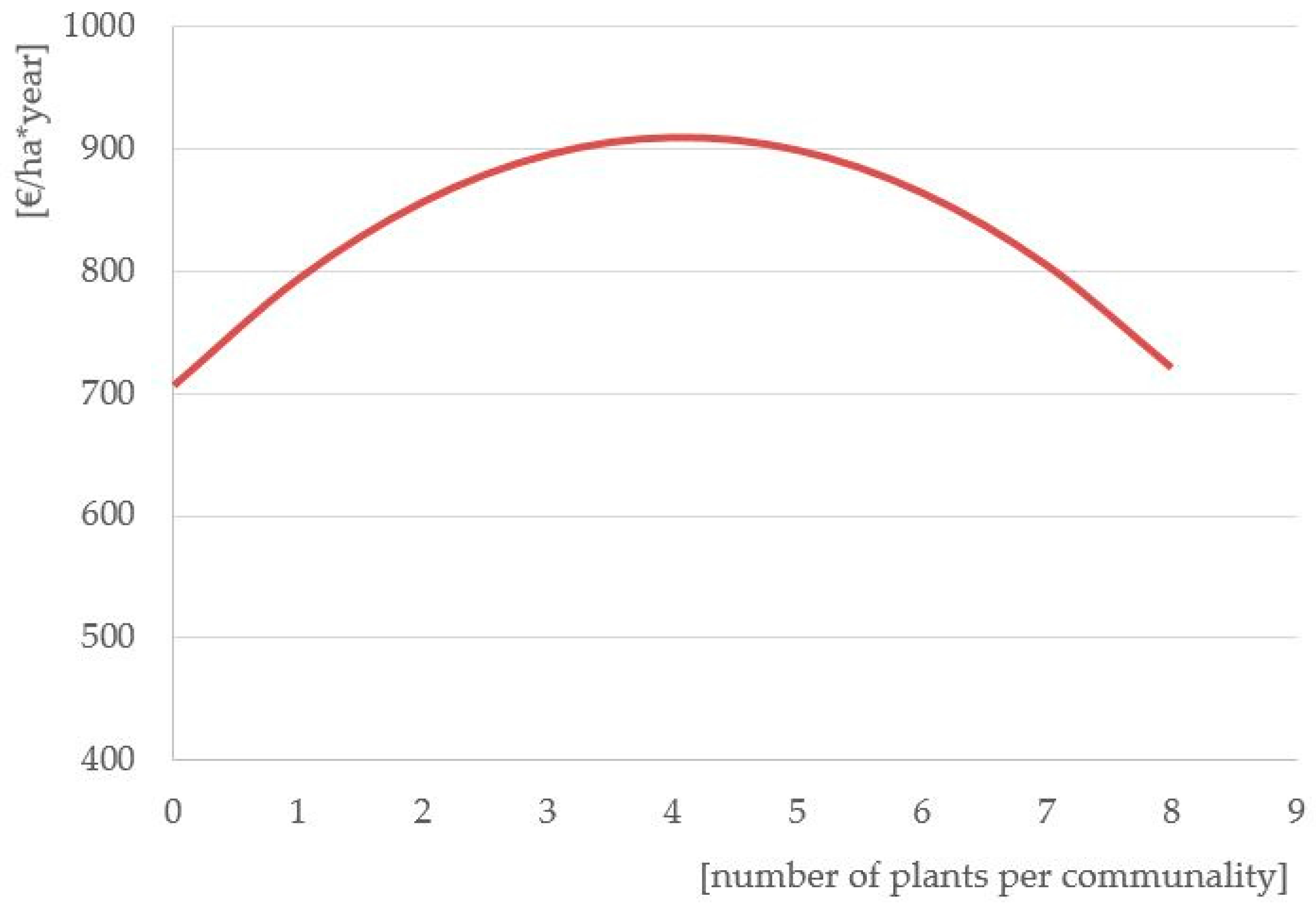
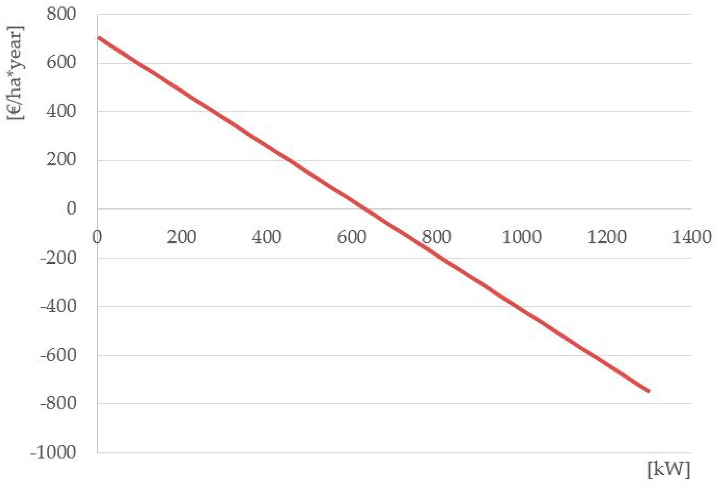
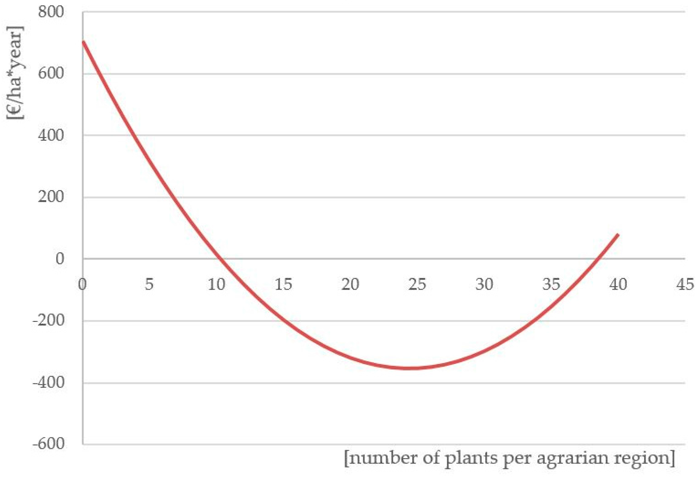
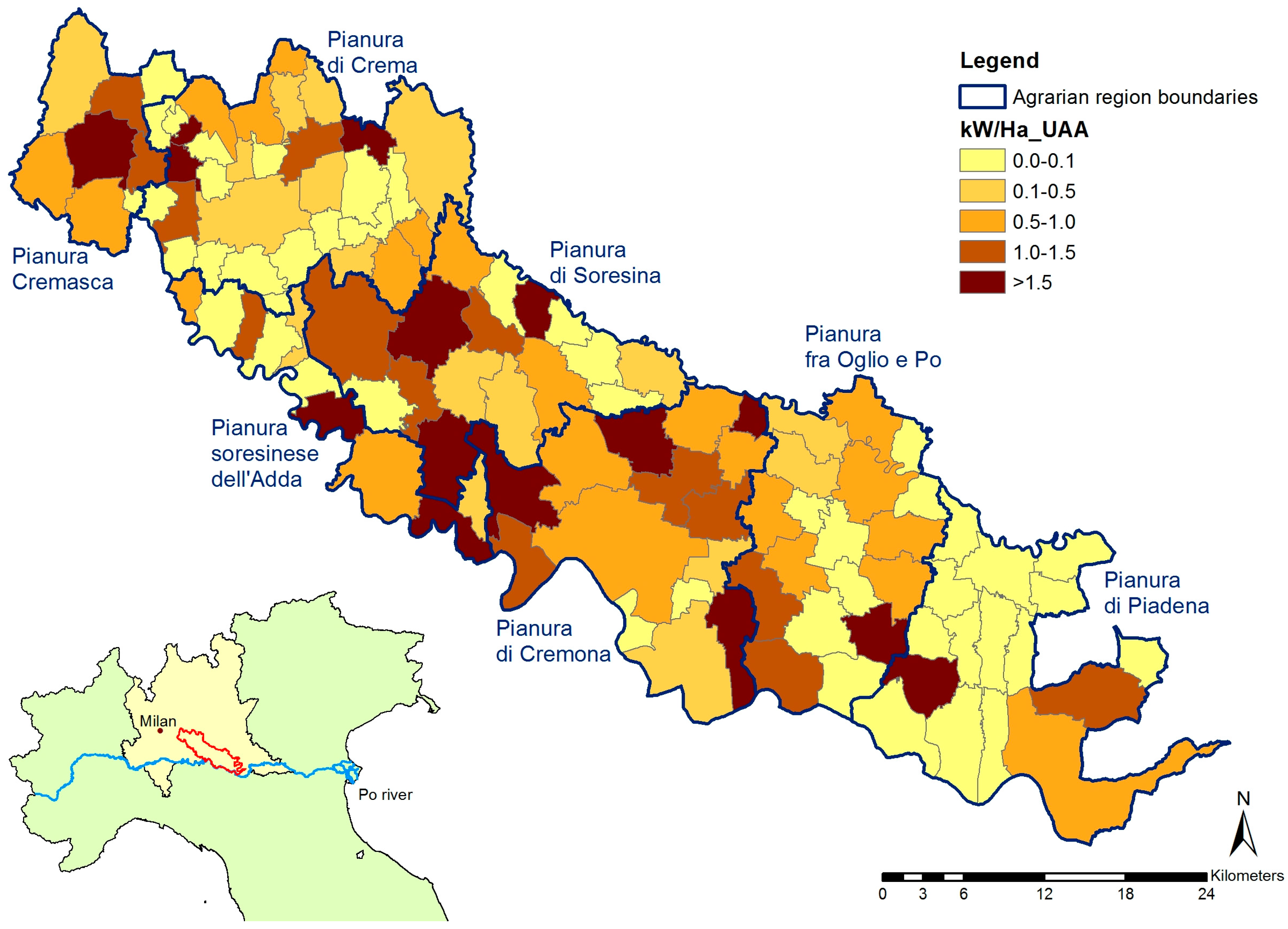
• Biogas plant data—give information about the quantity of plants and kW installed, the type of plants and their spatial distribution in the considered area. The number of plants and the kW installed approximate the dimension of the biogas sector (pl_m, pl_r, kw_m, and kw_r). These variables are expected to have a positive relationship with the price of the rented area, because they should approximate the quantity of energy crops (maize silage) requested and the effect of the shortage of available land [10]. Nonetheless, two more pieces information are needed to improve the description of this relationship. Firstly, it is known that different feedstock blends must be adopted depending on the technology of each plant, so we approximated differences in technology controlling for the average dimension of the plants (pp_m and pp_r). Secondly, as transport costs constrain energy crop provision [10,35], the distance of the plants from rented land has been approximated measuring the effect of kilowatts installed in the municipality and the agrarian regions the land rental contracts pertain to. This approximation of the distances between plants and rented land was an inevitable choice, due to the lack of georeferenced data.
  We used six variables to measure the impact of biogas production. They are a set of three variables, computed for two different buffers around each rental contract: at the municipal level (smaller buffer) and at the level of agricultural region (larger buffer). As the estimated model is not spatially explicit, the buffers are intended to account, indirectly, for the spatial effect of biogas plants on rental prices. The three variables considered, namely the number of plants (pl), nominal capacity per hectare (kw), and average size of the biogas plants (pp) used at different territorial levels (municipality and agrarian region) bring different information, even if correlated:

  ○

  The number of biogas plants in a given area (municipality, pl_m, or agrarian region, pl_r) affects the level of competition for feedstocks (manure, maize silage, or other crops). As shown in recent studies on biogas in the same area [10,35,36], the transport costs for biogas input and digestate spreading are non-linear, with an efficient ray of procurement that depends on plant size and feedstock mix. As spatial information on the location of rented land with respect to each biogas plant is missing, the model accounts for this feature by including the number of biogas plants in the surroundings of rented land. These variables capture the overlapping effect of efficient rays of feedstock procurement among biogas plants.

  ○

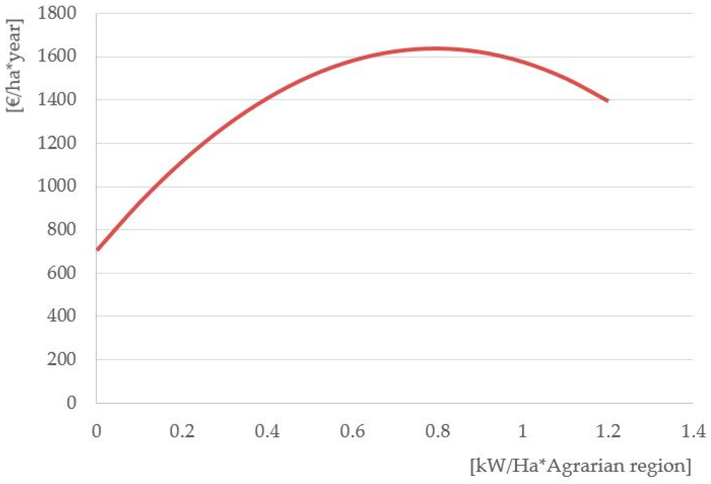
  The nominal capacity of biogas per hectare of UAA (municipality, kw_m, or agrarian region, kw_r) bring information on the density of the installed power and measure the demand for energy crops.

  ○

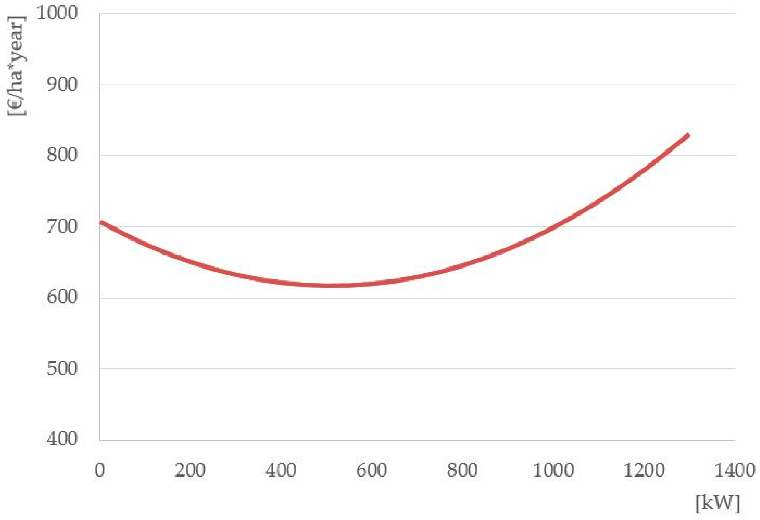
  The average size of biogas plants (municipality, pp_m, or agrarian region, pp_r) allows capturing the different technology of biogas production. In particular, small- and medium-sized biogas plants use larger proportions of manure and slurry that may decrease the value of land used for slurry location. On the other hand, large-sized plants are fed mainly with energy crops (maize silage), that may increase the demand of land for that purpose.

• Agricultural land use data—give information about farmers’ choices on land use and approximate if rented land is suited for the cultivation of certain crops. In our case, availability for maize and energy crops is expected to be directly related to the land rental price.
• Contract signature data—show when the contract was signed. This is considered relevant with reference to Italian subsidization schemes for biogas that changed in 2013 (according to Ministerial Decree 6 July 2012 [37]). The variable’s coefficient may change over years as an effect of change in policies. The institutional factors are decisive for the kind of biogas plants established, their scale, and the technology employed [25,26].
• Agrarian regions—represent a macro-statistic unit that groups municipalities having similar rural characteristics. As for land use data, different agrarian regions may have very different characteristics [38] that should be taken into account to control for unobserved spatial variability [16,31].

3.3. Estimation Strategy and Limitations of the Model

As mentioned, the hedonic price model presented in Section 3.1 has been estimated using OLS regression calculated with STATA (Stata Statistical Software Release 13.1, StataCorp LP, College Station, TX, USA, http://www.stata.com/). The regression has been firstly adjusted for heteroscedasticity using Huber-White sandwich estimators. Secondly, as land values may exhibit spatial correlation, it has been necessary to check for it. Moran’s I test has been used both on the dependent variable (each year and for the full sample used in the regression) and on the residuals of the regression (Model 5 in

Table 2. Explanatory variables for land rental price per year in ordinary least squares (OLS) models.

Variables	Model 1		Model 2		Model 3		Model 4		Model 5
	Biogas Variables at Municipality Level		Biogas Variables at Agrarian Region Level		Biogas Variables at Municipality Level w/out Nominal Capacity per ha		Biogas Variables at Agrarian Region Level w/out Nominal Capacity per ha		Biogas Variables at Municipality and Agrarian Region Level
R-squared	0.221		0.225		0.218		0.233		0.236
Rent value (Dependent)	Coefficient		Coefficient		Coefficient		Coefficient		Coefficient
Biogas variables
pl_m	95.146	***	-	-	86.870	**	90.728	**	99.324	***
pl_m2	−11.096	**	-	-	−11.605	**	−12.553	**	−12.189	**
kw_m	−102.594	-	-	-	-	-	-	-	−107.459	-
kw_m2	16.670	-	-	-	-	-	-	-	19.370	-
pp_m	−0.370	-	-	-	−0.428	*	−0.418	**	−0.353	*
pp_m2	0.000	**	-	-	0.000	*	0.000	**	0.000	**
pl_r	-	-	−82.401	**	-	-	−84.986	***	−86.974	***
pl_r2	-	-	1.704	**	-	-	1.758	**	1.784	***
kw_r	-	-	2324.436	**	-	-	2332.303	**	2348.650	**
kw_r2	-	-	−1477.331	**	-	-	−1482.357	**	−1478.670	**
pp_r	-	-	−1.209	**	-	-	−1.103	**	−1.120	**
pp_r2	-	-	0.001	*	-	-	0.001	-	0.001	-
liv	13.781	**	13.383	**	13.212	**	12.015	**	12.577	**
Agricultural land use—Reference = w&u_s
mai_s	282.483	*	245.839	-	281.272	*	263.700	-	262.627	-
ene_s	386.007	**	342.262	*	373.166	**	367.937	*	378.485	*
foa_s	332.679	**	288.864	*	332.186	**	306.245	*	304.234	*
fop_s	224.009	-	194.369	-	215.671	-	206.667	-	211.729	-
veg_s	399.413	**	354.481	*	401.833	**	379.191	**	374.293	**
vif_s	93,348.110	-	142,171.800	-	107,891.300	-	117,222.400	-	103,186.900	-
nur_s	896.572	**	847.957	**	889.587	**	893.461	**	896.782	**
Year—Reference = 2010
2011	125.392	-	207.114	**	126.026	*	203.974	**	209.924	**
2012	146.193	**	246.544	*	143.115	**	241.001	*	253.344	*
2013	106.542	***	204.394	-	101.886	**	202.458	-	217.887	-
2014	115.008	**	181.913	-	110.063	**	184.284	-	200.543	-
Agrarian Region—Reference = 19-07
19-01	−103.537	***	−210.684	-	−108.647	***	−203.130	-	−200.241	-
19-02	6.241	-	153.985	-	3.754	-	171.681	-	186.836	-
19-03	90.899	***	−23.887	-	81.185	***	−20.397	-	−17.447	-
19-04	−8.317	-	97.430	-	−6.976	-	108.883	-	117.896	-
19-05	22.185	-	170.505	-	16.111	-	175.220	-	186.905	-
19-06	−47.948	*	113.103	-	−54.068	*	122.238	-	137.390	-
const	368.818	**	744.100	***	392.240	**	726.699	***	706.983	***
------ for control variables see Appendix D ------

Note: Sign. * = 0.10; ** = 0.05; *** = 0.01.

in the next section), as its results allow rejecting the presence of spatial correlation or considering negligible the magnitude of such a feature.

The effect of biogas on land prices has been tested using a polynomial specification (variable in level and squared) to capture non-linear effects. The rationale behind using such a functional form relies on specific features of biogas production. These are non-linear transportation costs of input (energy crops and slurry) and output (digestate), as outlined in studies carried out in the same area [10,35,36]. Thus, it is plausible to assume that the non-linearity in transportation costs may translate in non-linear effects of biogas on rental prices. In order to check the reliability of the non-linear relationships among dependent and biogas variables, a Ramsey’s RESET test and an F-test of joint non-significance of biogas parameter estimates have been performed. The joint results of these tests indicate the linear-polynomial as an acceptable specification.

The robustness of the abovementioned regression strategy may be affected by missing data on soil quality at an adequate scale (parcel/contract level). Unlike other papers in the same field [18] we do not have data on soil quality at the parcel level; our data, (classified according to land capability using the United State Department of Agriculture (USDA) soil taxonomy), are rendered to a scale (1:50,000) that does not allow enough variability within the area examined. As soil quality is an important attribute of land value, its exclusion from our hedonic model may lead to biased estimates of other attributes. Such distortion may be mitigated by including land uses in the model. It is intuitive, in fact, that land use and soil quality are correlated, to some extent. The same issue applies to relevant data that are available at the province level, such as macroeconomic variables as classified according to Feichtinger and Salhofer [11].

A final relevant limitation deserves to be mentioned. Farmland can be used for many crops and land values are simultaneously in equilibrium with food, feed, and bioenergy markets. An increased demand of land for energy purposes incurs competition with alternative, uses such as maize for livestock feeding, pushing-up land values. However, this causal effect may actually be counterbalanced by the import of maize from other countries. Due to the lack of data, we could not control for this effect.

4. Results and Discussion

Considering the focus of the analysis, five different HP models have been used in order to test the stability in sign, significance, and magnitude of parameter estimates of OLS. Table 2 shows the variability of land rental prices due to biogas plants and livestock density (as they compete for land use), agricultural land use, year of signature of the contract, and location of the rented land. The parameter estimates of other control variables are reported in Appendix D. The five specifications have the same combination of control variables and differ for groups of biogas variables. Model 1 and Model 2 report biogas variables at municipality and agrarian region level, respectively. Model 3 includes significant biogas variables of Model 1 only, and Model 4 includes all significant variables at both municipal and agrarian region levels. Finally, all of the biogas variables enter Model 5. As the regression outcomes are stable in terms of the coefficients’ values and significance of the explanatory variable across the five specifications, we will comment on the results of Model 5 because it is more comprehensive.

According to Model 5’s results, the regression has run on 812 land rental contracts against the 2063 available, because the econometric package dropped all of those observations missing at least one of the variables considered in the model. Table 2 shows that the land rental price is positively influenced by the livestock density and the agricultural land use for energy crops, forage alternation, vegetables, and plant nursery. The first two years of contracts considered show the same relationship, while the agrarian region of pertinence of the rent contract does not influence the dependent variable. Among the control variables, the dimension of rented area and the presence of Common Agricultural Policy (CAP) subsidies affect the rental land price significantly and positively. Considering the farming type, the livestock farm tenant is willing to pay more for land rent (from 106.3 to 709.5 €/ha) compared to dairy farms (reference). A notable exception is represented by specialist goat farms that probably rent marginal lands for grazing. Among the non-significant control variables are the length of the contract, the share of UAA within the municipality (rurality), the presence of rural building in the contract, the standard output of the tenant, the presence of second crops, and the type of land owner.

Considering the focus of this paper, the effects of biogas plant characteristics on the dependent variable are the most relevant findings of the empirical analysis. Results show the significant relation between the number of plants and the average installed kW per plant in the municipality and agrarian region of the contract. Furthermore, the land rental price is linked to the kW per hectare of the agricultural utilized area in the agrarian region, which is not confirmed at the municipal level. As explained, these variables are used to approximate the effect of technology of the biogas plants (plant’s average size, pp), the demand for maize silage for bioenergy production with respect to the number of plants (number of plants, pl, and nominal capacity, kW), and the transportation costs of the energy crops from fields to plants (municipal vs. agrarian region location of the rented land; _m and _r suffixes, respectively).

Model 5 shows that biogas plants have a non-linear type effect on the rental land price according to the power (pl and kW), the technologies used for the production of biogas (pp), and the distance between the plants and the rented land. These trends, shown in the Figure 2, Figure 3, Figure 4, Figure 5 and Figure 6, are in line with the expected results with regards to the growing branches of the functions estimated. In fact, it does make sense that land rental prices rise as the demand for land for energy crops (maize silage) increases.

On the contrary, the depressive effects of biogas on the price of land rent may be counterintuitive and worth careful comment. In particular, Figure 2 shows that the rent in the agrarian region increases to a value of 0.8 kW/ha installed power per hectare, then it starts to decrease. This bell-shaped trend presumably derives from a sequence of interconnected events: increasing levels of kW installed per hectare fosters the competition for energy crops, forcing producers to search for feedstock from more and more distant areas and pushing up the cost of bioenergy input procurement [10,36]. Beyond a certain threshold of installed power density, the competition for local land becomes economically unviable and leads producers to shift from maize silage (which is bulky) to other biogas feedstocks. Such alternative inputs may be local by-products deriving from agricultural, food, agro-industrial, and forestry industries (as allowed by Ministerial Decree 6 July 2012 [37]) and/or imported biomass, which would explain the downward trend of rental prices for high kW/ha values. This hypothesis could also explain the decreasing trend described in Figure 3.

The descending branches of the u-shaped curves, conversely, represents a somehow unexpected effect. It may be explained by the possibility of postponement of manure spreading which reduces the demand for land, decreasing its rental value, as in the Figure 4. This phenomenon is linked to the biogas technology applied and is more pronounced in large areas as agricultural regions (Figure 5) where we observed only a negative linear effect. A similar explanation may also apply to Figure 6, which relates the rental land price and the number of existing biogas plants in the agrarian region. In particular, the price of land decreases to an average density of 24 plants because of the delay of the timing of manure spreading. With the increase of the number of plants, it starts to increase, as the effect of competition for arable land becomes prevalent. The fact that the graph goes into the negative range is not surprising, since these plots are used to describe the "pure" effect of the variable on the rental amount.

Furthermore, we interpreted the positive and significant relationships between land rental price and livestock pressure per hectares, land utilization for forage alternation, arable and energy crops as a proof for competition between food, feed, and fuel. This would confirm the relevance of the “environment trilemma” for social and economic sustainability of bioenergy that need to exploit agricultural land to be produced. Additionally, we observe a statistically significant increase in rental prices for contracts signed in 2011 and 2012, compared to 2010 (reference year). On the contrary, in 2013 and 2014 such an effect is not significant. This may be the result of a change in biogas policy that occurred exactly at the end of 2012. In particular, the Decree of 6 July 2012 [37] established a new subsidization scheme aimed at providing more incentives for smaller sized plants and for those using agro-food by-products (the mentioned plants were in the following size ranges: 1–300 kW, 301–600 kW, and over 601 kW [35]). Therefore, while until the end of 2012 mainly large-sized plants were running using maize silage, contributing for more pressure on land rental prices, from 2013 new policies downturned the previous trend.

Finally, it is worth noting that coefficients of determination R² of the model account for the 23.6% of the variance, which means that the combination of dependent variables included in the model explain a limited amount of variability in the dependent variable, as compared to previous studies. Such low values in R² may be due to the lack of information on soil quality, as explained in Section 3.3. Furthermore, this limitation must be considered together with the peculiarities of the agricultural land market. In fact, many drivers of land rental prices are difficult to be considered in the model because of their nature. For example, the effect of human capital of both tenants and land owners may capture information on characteristics of the relationships between the two parties. The presence and nature of special clauses or verbal agreements do not enter the model because they are often non-reported in the contract and, thus, out of reach for the researcher. All these factors considered, we are still moderately optimistic in evaluating the reliability of the OLS results because of the stability shown by different specifications and the accordance with expected results.

5. Conclusions and Policy Implications

In recent years, agricultural economists published a fair amount of studies dealing with the analysis of the drivers of the agricultural land market. Obviously, these studies are constrained by data availability and quality, thus researchers from different countries may possess some relevant information and lack some others. The consequence is two-fold. On the one hand, the findings that come from different data and econometric models suffer for repeatability and cannot be formally confirmed (nor rejected). On the other hand, any scientifically-grounded and sound study on the land market may potentially shed new light on this topic and significantly contribute to the accumulation of specific knowledge on this field.

The present paper focused on the relationship between land rental prices and biogas production (in terms of installed power, number and size of plants). We start from the simple observation that biogas plants use some crops as feedstock to produce energy, thus representing a new source of competition for land access. This is expected to affect the price of land rental. Specifically, the rationale would be predicting a positive relation between installed kilowatt of biogas per agricultural area and land rental price. Nonetheless, this expected phenomenon may take different shapes and intensities, as the demand of bioenergy crops (and then the impact on land price) depends on a variety of features [39], likes plant size, feedstock mix, and the transportation costs of bioenergy crops from fields to plants [10].

We measured this phenomenon applying a hedonic price model in a case study area in Northern Italy that was previously proven to be relevant for biogas plant installation [9]. We found that installed power per hectare, number of plants, and average plant size significantly affect land rental prices in a nonlinear fashion. Furthermore, such effects take different shapes according to the territorial level to which the biogas feature operates (municipal or agrarian region). Such detected nonlinear effects suggest that technologies and distances between the biogas plants and the rural area devoted to energy crop production matter in determining the land rental price.

These findings may be considered socially and scientifically relevant because we measured the thresholds for a significant effect of biogas plants characteristics on land rental prices, which could be very useful for a bioenergy regulatory plan design. Considering that a policy-maker may be interested in protecting food and feed production against excess competition exerted by bioenergy crops, we identified a way to calculate the levels of kW per hectares and/or the best biogas plant’s dimensions that help to reach this objective. Consequently, these results and the procedure could be applied to set the parameters to incentivize the most efficient bioenergy policy in rural areas. Furthermore, we confirm previous evidence on the outcome of different biogas incentive schemes; as pointed out by Bartoli et al. [10], subsidizing large-sized plants (that use mainly energy crops) would lead to increased competition for land, while when small- and medium-sized plants (using prevalently manure) are incentivized, such pressure on agricultural land would be reduced. Our findings are in line with this hypothesis, as we estimated an increase in land rental prices only in those years (2010 and 2011) where the large-sized plants were more subsidized, while such an effect is not significant over the subsequent years (2013 and 2014) with the withdrawal of the old policy scheme.

For example, considering our case study, the findings indicate that the smallest and largest biogas plants give the best social performance, i.e., they impact less on land rental prices. This seems to be the basis for an optimal win-win policy based in incentivizing (1) small plants using livestock manures, which helps breeders maintain adequate environmental standards without increasing their feed cost; and (2) large plants using agro-food by-products, that need professionals to be consulted to optimize the recycle of food waste restoring the nitrogen and phosphorus cycles. These considerations are in line with evidence provided by biophysical economists on the feasibility of maize-based bioenergy. The researchers, using non-monetary metrics, proved, in fact, that the bioenergy industry is unsustainable when using agricultural commodities as energy inputs [40], while it is a desirable option when using by-products both in social and energy efficiency terms [41]. Finally, the limitations discussed in Section 3.3 deserve to be recalled. The lack of information, especially on soil quality, macroeconomic factors and the import of agricultural commodities, suggests that our results omit some relevant effects on land rental prices. From another viewpoint, these shortcomings may be considered valuable recommendations for further studies.

References

1. Böhringer, C.; Keller, A.; Van der Werf, E. Are green hopes too rosy? Employment and welfare impacts of renewable energy promotion. Energy Econ. 2013, 36, 277–285. [Google Scholar] [CrossRef]
2. Tilman, D.; Socolow, R.; Foley, J.A.; Hill, J.; Larson, E.; Lynd, L.; Pacala, S.; Reilly, J.; Searchinger, T.; Somerville, C.; et al. Beneficial biofuels—The food, energy and environment trilemma. Science 2009, 325, 270–271. [Google Scholar] [CrossRef] [PubMed]
3. Harvey, M.; Pilgrim, S. The new competition for land: Food, energy, and climate change. Food Policy 2011, 36, 40–51. [Google Scholar] [CrossRef]
4. Murphy, R.; Woods, J.; Black, M.; McManus, M. Global developments in the competition for land from biofuels. Food Policy 2011, 36, 52–61. [Google Scholar] [CrossRef]
5. Rathmann, R.; Szklo, A.; Schaeffer, R. Land use competition for production of food and liquid biofuels: An analysis of the arguments in the current debate. Renew. Energy 2010, 35, 14–22. [Google Scholar] [CrossRef]
6. Dornburg, V.; van Vuuren, D.; van de Ven, G.; Langeveld, H.; Meeusen, M.; Banse, M.; van Oorschot, M.; Ros, J.; van den Born, G.J.; Aiking, H.; et al. Bioenergy revisited: Key factors in global potentials of bioenergy. Energy Environ. Sci. 2010, 3, 258–267. [Google Scholar] [CrossRef]
7. Gelfand, I.; Sahajpal, R.; Zhang, X.; Izaurralde, R.C.; Gross, K.L.; Robertson, G.P. Sustainable bioenergy production from marginal lands in the US Midwest. Nature 2013, 493, 514–517. [Google Scholar] [CrossRef] [PubMed]
8. Sgroi, F.; Foderà, M.; Di Trapani, A.M.; Tudisca, S.; Testa, R. Economic evaluation of biogas plant size utilizing giant reed. Renew. Sustain. Energy Rev. 2015, 49, 403–409. [Google Scholar] [CrossRef]
9. Mela, G.; Canali, G. How distorting policies can affect energy efficiency and sustainability: The case of biogas production in the Po Valley (Italy). AgBioForum 2014, 16, 194–206. [Google Scholar]
10. Bartoli, A.; Cavicchioli, D.; Kremmydas, D.; Rozakis, S.; Olper, A. The Impact of Different Energy Policy Options on Feedstock Price and Land Demand for Maize Silage: The Case of Biogas in Lombardy. Energy Policy 2016, 96, 351–363. [Google Scholar] [CrossRef]
11. Feichtinger, P.; Salhofer, K. What Do We Know about the Influence of Agricultural Support on Agricultural Land Prices? Ger. J. Agric. Econ. 2013, 62, 71–85. [Google Scholar]
12. März, A.; Klein, N.; Kneib, T.; Musshoff, O. Analysing farmland rental rates using Bayesian geoadditive quantile regression. Eur. Rev. Agric. Econ. 2015, 3, 1–36. [Google Scholar] [CrossRef]
13. Guastella, G.; Moro, D.; Sckokai, P.; Veneziani, M. The capitalization of area payments into land rental prices: A panel sample selection approach. In Proceedings of the 2014 International Congress, European Association of Agricultural Economists (EAAE), Ljubljana, Slovenia, 26–29 August 2014.
14. Latruffe, L.; Le Mouël, C. Capitalization of government support in agricultural land prices: What do we know? J. Econ. Surv. 2009, 23, 659–691. [Google Scholar] [CrossRef]
15. Bartolini, F.; Viaggi, D. The common agricultural policy and the determinants of changes in EU farm size. Land Use Policy 2013, 31, 126–135. [Google Scholar] [CrossRef]
16. Kilian, S.; Antón, J.; Salhofer, K.; Röder, N. Impacts of 2003 CAP reform on land rental prices and capitalization. Land Use Policy 2012, 29, 789–797. [Google Scholar] [CrossRef]
17. Karlsson, J.; Nilsson, P. Capitalisation of Single Farm Payment on farm price: An analysis of Swedish farm prices using farm-level data. Eur. Rev. Agric. Econ. 2014, 41, 279–300. [Google Scholar] [CrossRef]
18. Feichtinger, P.; Salhofer, K. The Fischler reform of the common agricultural policy and agricultural land prices. Land Econ. 2016, 92, 411–432. [Google Scholar] [CrossRef]
19. Duvivier, R.; Gaspart, F.; de Frahan, B.H. A panel data analysis of the determinants of farmland price: An application to the effects of the 1992 CAP reform in Belgium. In Proceedings of the XIth EAAE Congress on “The Future of Rural Europe in the Global Agri-Food System”, Copenhagen, Denmark, 23–27 August 2005.
20. Pyykkonen, P. Spatial analysis of factors affecting Finnish farmland prices. In Proceedings of the 2005 International Congress, European Association of Agricultural Economists, Copenhagen, Denmark, 23–27 August 2005.
21. Folland, S.T.; Hough, R.R. Nuclear power plants and the value of agricultural land. Land Econ. 1991, 67, 30–36. [Google Scholar] [CrossRef]
22. Morehart, M.; Kuethe, T.; Beckman, J.; Ifft, J.; Williams, R. Trends in US Farmland Values and Ownership; US Department of Agriculture, Economic Research Service: Washington, DC, USA, 2012.
23. Borchers, A.; Ifft, J.; Kuethe, T. Linking the price of agricultural land to use values and amenities. Am. J. Agric. Econ. 2014, 96, 1307–1320. [Google Scholar] [CrossRef]
24. Swinnen, J.; Ciaian, P.; Kancs, D.A. Study on the Functioning of Land Markets in the EU Member States under the Influence of Measures Applied under the Common Agricultural Policy; Unpublished Report to the European Commission; Centre for European Policy Studies: Brussels, Belgium, 2008. [Google Scholar]
25. Carrosio, G. Energy production from biogas in the Italian countryside: Policies and organizational models. Energy Policy 2013, 63, 3–9. [Google Scholar] [CrossRef]
26. Carrosio, G. Energy production from biogas in the Italian countryside: Modernization vs. repeasantization. Biomass Bioenergy 2014, 70, 141–148. [Google Scholar] [CrossRef]
27. Johansson, D.J.; Azar, C. A scenario based analysis of land competition between food and bioenergy production in the US. Clim. Chang. 2007, 82, 267–291. [Google Scholar] [CrossRef]
28. Ostermeyer, A.; Schönau, F. Effects of biogas production on inter-and in-farm competition. In Proceedings of the 131th EAAE Seminar ‘Innovation for Agricultural Competitiveness and Sustainability of Rural Areas’, Prague, Czech Republic, 18–19 September 2012.
29. Appel, F.; Ostermeyer-Wiethaup, A.; Balmann, A. Effects of the German Renewable Energy Act on structural change in agriculture—The case of biogas. Utilities Policy 2016, 41, 172–182. [Google Scholar] [CrossRef]
30. Emmann, C.H.; Guenther-Lübbers, W.; Theuvsen, L. Impacts of biogas production on the production factors land and labour–current effects, possible consequences and further research needs. Int. J. Food Syst. Dyn. 2013, 4, 38–50. [Google Scholar]
31. Hüttel, S.; Odening, M.; Kataria, K.; Balmann, A. Price Formation on Land Market Auctions in East Germany—An Empirical Analysis. Ger. J. Agric. Econ. 2013, 62, 99–115. [Google Scholar]
32. Lancaster, K.J. A new approach to consumer theory. J. Political Econ. 1966, 74, 132–157. [Google Scholar] [CrossRef]
33. Rosen, S. Hedonic prices and implicit markets: Product differentiation in pure competition. J. Political Econ. 1974, 82, 34–55. [Google Scholar] [CrossRef]
34. Vaccari, V.; Manco, I.; Cordoni, C.; Valvassori, A. Features and sustainability components of a laboratory of analysis for biogas plants. Econ. Aziend. Online 2015, 6, 35–42. [Google Scholar]
35. Gaviglio, A.; Pirazzoli, C.; Ragazzoni, A. Zootecnia e Biogas—Incentivi 2013, 100 Pagine per Capire; Edizioni L’Informatore Agrario: Verona, Italy, 2013. [Google Scholar]
36. Gaviglio, A.; Pecorino, B.; Ragazzoni, A. Produrre energia rinnovabile nelle aziende agro-zootecniche. Effetti economici dalle novità introdotte nella normativa del 2012. Econ. Agro-Aliment. 2014, 16, 31–60. [Google Scholar] [CrossRef]
37. Implementation of Art. 24 of Legislative Decree of 3 March 2011, n. 28, Containing Incentives for the Production of Electricity from Renewable Sources by Installations at Various PV; Ministerial Decree 6 July 2012. Available online: http://www.sviluppoeconomico.gov.it/images/stories/normativa/DM_6_luglio_2012_sf.pdf (accessed on 10 May 2016).
38. Demartini, E.; Gaviglio, A.; Bertoni, D. Integrating agricultural sustainability into policy planning: A geo-referenced framework based on Rough Set theory. Environ. Sci. Policy 2015, 54, 226–239. [Google Scholar] [CrossRef]
39. Pöschl, M.; Ward, S.; Owende, P. Evaluation of energy efficiency of various biogas production and utilization pathways. Appl. Energy 2010, 87, 3305–3321. [Google Scholar] [CrossRef]
40. Murphy, D.J.; Hall, C.A.; Powers, B. New perspectives on the energy return on (energy) investment (EROI) of corn ethanol. Environ. Dev. Sustain. 2011, 13, 179–202. [Google Scholar] [CrossRef]
41. Arodudu, O.; Voinov, A.; van Duren, I. Assessing bioenergy potential in rural areas—A NEG-EROEI approach. Biomass Bioenergy 2013, 58, 350–364. [Google Scholar] [CrossRef]
42. Angrist, J.D.; Pischke, J.S. Mostly Harmless Econometrics: An Empiricist’s Companion; Princeton University Press: Princeton, NJ, USA, 2008. [Google Scholar]
43. Wooldridge, J.M. Econometric Analysis of Cross Section and Panel Data; MIT Press: Cambridge, MA, USA, 2010. [Google Scholar]
44. Wooldridge, J.M. Introductory Econometrics: A Modern Approach; Nelson Education: Toronto, ON, Canada, 2015. [Google Scholar]
Figure 1. The Province of Cremona in the Lombardy Region and the distribution of biogas plants in the area.
Energies 09 00965 g001
Figure 2. Function of installed kilowatt per hectare in the agrarian region on rental price (kw_r).
Energies 09 00965 g002
Figure 3. Function of number of biogas plants in a municipality on rental price (pl_m).
Energies 09 00965 g003
Figure 4. Function of the average plants’ power in a municipality on rental price (pp_m).
Energies 09 00965 g004
Figure 5. Function of the average plants’ power in the agrarian region on rental price (pp_r).
Energies 09 00965 g005
Figure 6. Function of the number of biogas plants in the agrarian region on rental price (pl_r).
Energies 09 00965 g006