Article

A Detailed Assessment of the Wave Energy Resource at the Atlantic Marine Energy Test Site

1
College of Engineering and Informatics, National University of Ireland, Galway, Ireland
2
Centre for Marine and Renewable Energy Ireland (MaREI), Galway, Ireland
3
Ryan Institute for Environmental, Marine and Energy Research, Galway, Ireland
*
Author to whom correspondence should be addressed.
Energies 2016, 9(11), 967; https://doi.org/10.3390/en9110967
Submission received: 18 July 2016 / Revised: 7 November 2016 / Accepted: 9 November 2016 / Published: 18 November 2016
(This article belongs to the Special Issue Numerical Modelling of Wave and Tidal Energy)

Abstract

:
Wave characteristic assessments of wave energy test sites provide a greater understanding of prevailing wave conditions and are therefore extremely important to both wave energy test site operators and clients as they can inform wave energy converter design, optimisation, deployment, operation and maintenance. This research presents an assessment of the wave resource at the Atlantic Marine Energy Test Site (AMETS) on the west coast of Ireland based on 12-years of modelled data from January 2004 to December 2015. The primary aim is to provide an assessment of annual and seasonal wave characteristics and resource variability at the two deployment berths which comprise the site. A nested model has been developed using Simulating WAves Nearshore (SWAN) to replicate wave propagations from regional to local scale with a 0.05° resolution model covering the northeast Atlantic and a 0.0027° resolution model covering AMETS. The coarse and fine models have been extensively validated against available measured data within Irish waters. 12-year model outputs from the high resolution model were analysed to determine mean and maximum conditions and operational, high and extreme event conditions for significant wave height, energy period and power. Annual and seasonal analyses are presented. The 12-year annual mean P were 68 kW/m at Berth A (BA) and 57 kW/m at Berth B (BB). The resource shows strong seasonal and annual variations and the winter mean power levels were found to be strongly correlated with the North Atlantic Oscillation (NAO).

1. Introduction

The assessment of wave characteristics and wave energy resource at a specific location or area is necessary to determine an available wave resource with regard to wave energy harvesting. Furthermore, an understanding of wave characteristics as well as extreme wave events is critical for the engineering design of wave energy converters (WECs), especially for survivability as severe loadings on WECs can result from extreme wave events [1]. A minimum 10 years of data is recommended [2] for a wave resource assessment analysis. The primary aim of this research is an assessment of wave characteristics and wave energy resource at the Atlantic Marine Energy Test Site (AMETS) on the west coast of Ireland. 12-year high resolution modelled data for the period of January 2004 to December 2015 was used to carry out the assessment.
Wave energy harvesting has become a major interest in Ireland. The typical annual average power resources of deep water waves around the globe (based on hindcast modelled data generated by the National Oceanic and Atmospheric Administration (NOAA) Wave Watch III (NWW3) wind wave model for the 10 year period from 1997 to 2006) vary from 30 to 70 kW/m wave crest with a peak of 100 kW/m in the north-eastern Atlantic Ocean (AO) [3,4]. The geography and climatology of Ireland contribute to the formation of high wave events within Irish waters, particularly on the west coast [5]. The exposure to the AO and prevailing westerly winds contribute to swell wave propagations that travel more than three thousand miles across the AO before they reach Ireland’s west coast. Strong coastal winds contribute additional local wave generation. López et al. [6] showed the wave power level around Ireland varying in the range of 53–76 kW/m annually where annual wave power close to the AMETS location is in the region of 70 kW/m. Hence, it can be concluded that Ireland is an area with high wave power resources. Based on statistical analysis of the 10-year WorldWaves time series for the period of 1997–2006 [7], annual means of significant wave height (Hs) values in the AO are up to 4 m, while off the west coast of Ireland they vary from 2.5 m up to 3.5 m. Thus, it is evident that Ireland, and particularly the West coast of Ireland, is situated in a highly active wave zone. The most recent highest wave recorded in Ireland was 25 m on 12 February 2014, which was measured at Kinsale Energy Gas Platform (8 W, 51.367 N; see Figure 1), approximately 50 km off the south coast of Cork. The previous record wave height of 23.4 m was measured at Donegal M4 wave buoy off the northwest coast (9.992 W, 54.998 N; see Figure 1) on 26 January 2014 [8]. A detailed assessment of historical extreme wave events in Ireland is presented in [5] who divide these events into three categories—storm waves, tsunamis waves and rogue waves. The focus of the present research is to investigate the characteristics of wind-generated wave events, thus only storm waves are examined; tsunamis and rogue waves are not considered.
As evidence of Ireland’s interest in wave energy, there are two existing test sites for WECs on Ireland’s west coast [9]—the 1/4-scale Galway Bay test site (GBTS) (9.067 W, 53.249 N; see Figure 1) and the full-scale AMETS at Belmullet (9.991 W, 54.225 N; see Figure 1). A third site off the west coast of County Clare is the focus of the Westwave demonstration project (9.52 W, 52.775 N; see Figure 1), which aims to deploy five wave energy devices by 2018 in a move towards commercialisation of wave power generation. The site of interest in this research, AMETS, is exposed directly to the north-eastern AO, as shown in Figure 1. The wave climate in the area is influenced by variable weather conditions [10], as well as local geography and bathymetry [11]. The site comprises two deployment berths:
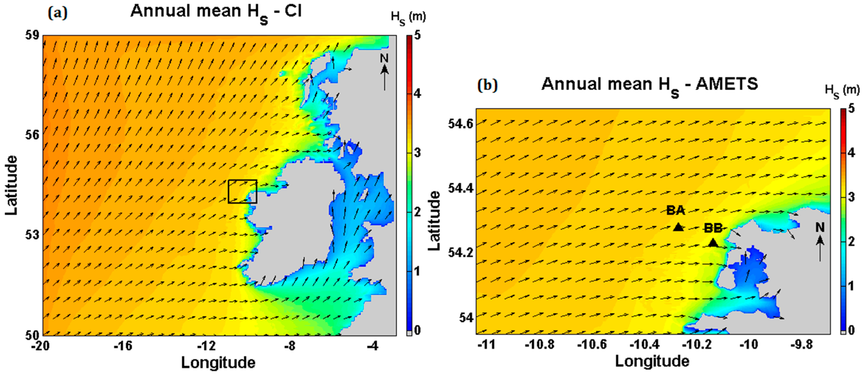
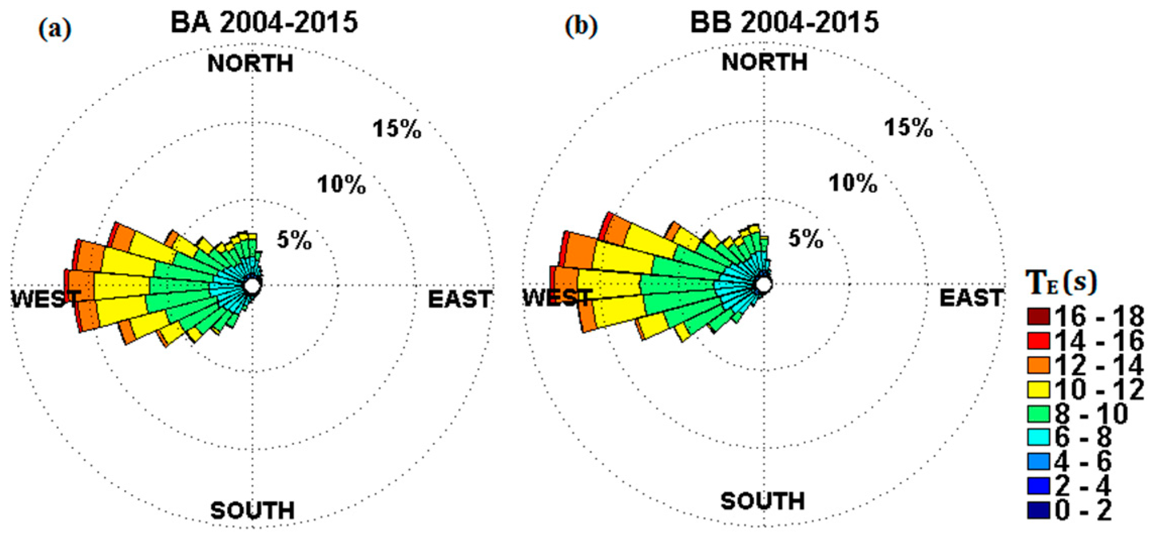
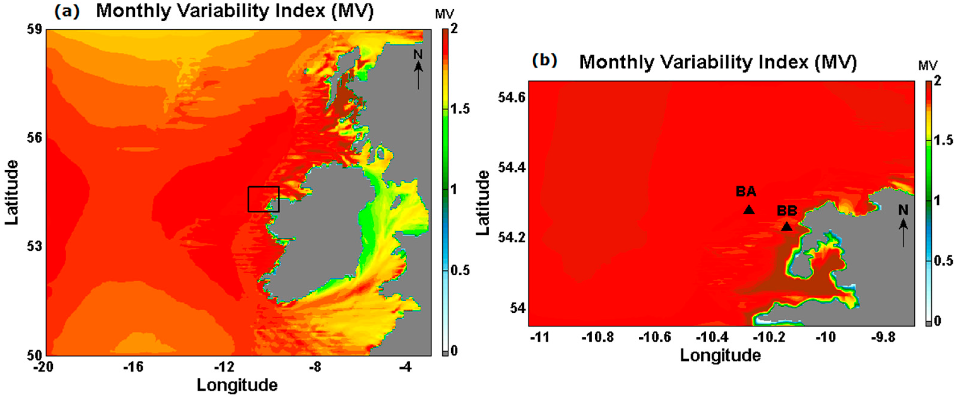
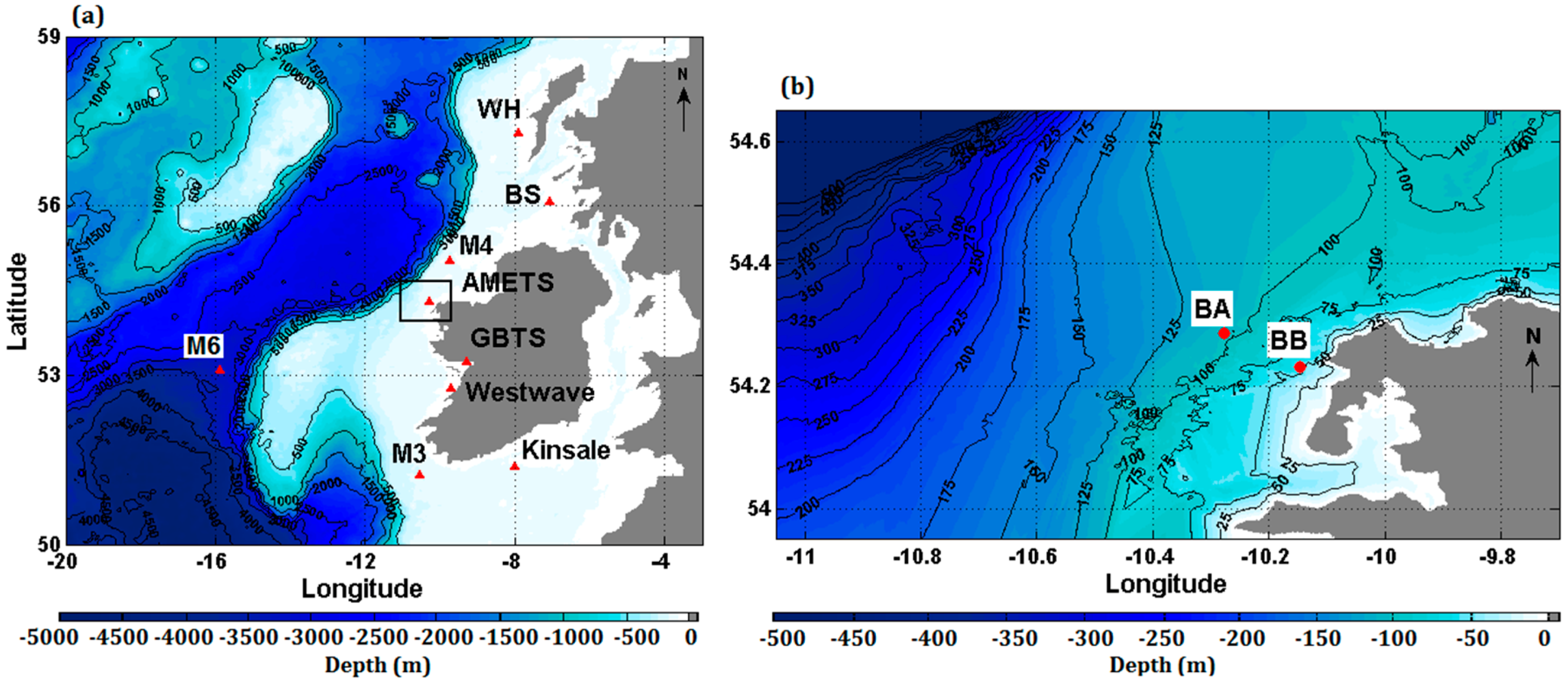
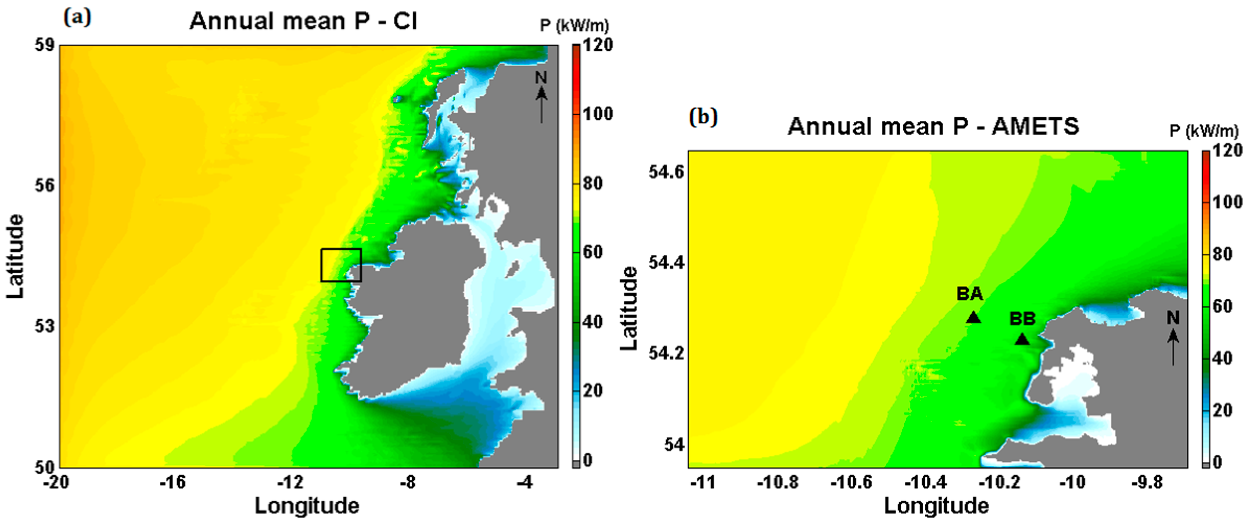
  • Berth A (BA): approximately 16 km offshore, 100 m water depth, and covering 6.9 km2;
  • Berth B (BB): approximately 6 km offshore, 50 m water depth, and covering 1.5 km2.
The main objective of the research is the assessment of wave characteristics and wave energy resource at AMETS. In the absence of long-term measured data, 12 years of high resolution modelled data were used. This required the development of a numerical wave model where a nesting application was implemented in which waves for a larger regional area were first simulated with a coarse grid wave model and then downscaled into a finer grid wave model for a smaller local area including AMETS. The boundary conditions for the fine grid model are derived from the coarse grid computation. The models were calibrated and validated against available measured data. The models were used to hindcast the period January 2004–December 2015 and a detailed assessment was conducted at both berths using the data from the high resolution (300 m) model which was output at 30 min intervals.
A previous wave resource assessment at AMETS [12], based on 15 years of modelled data for the years 1995–2009, calculated mean values of deep water wave power of 77 kW/m at BA and 62 kW/m BB. There are significant differences between the former and present study. The model of [12] was only validated for a short 1-month period, and only at BB, while the authors high resolution model is validated for much longer periods at both BA (2012–2013) and BB (2010–2013). The present model is shown to be more accurate than its predecessor and should therefore provide a more accurate characterisation of the wave resource at AMETS. The present study is also much more extensive than its predecessor; wave parameters (significant wave height (Hs), wave energy period (TE) and wave power (P)) are characterised for operational, high and extreme conditions, inter-annual and seasonal analyses are conducted, joint wave occurrence for the 12-year assessment period is presented, and detailed spatial map analyses are presented, none of which were included in [12]. The paper is laid out as follows. An overview of the model development and validation is described in Section 2. The results of the detailed assessments of Hs, TE, and P are presented in Section 3 along with a short discussion. Finally, the conclusions from the research are presented in Section 4.

2. Material and Methods

2.1. Wave Model Description

Numerical modelling methods have been widely used for decades to replicate ocean wave conditions at different scales and locations. Several numerical wave models such as the Wave Modelling (WAM) wave model [13], Wave Watch III (WW3) wave model [14], MIKE21 spectral wave model [15] and Simulating WAves Nearshore (SWAN) [16] wave model are available for use in hindcasting and forecasting wave conditions. These models use full wave spectra based on the integration of the wave energy (or alternatively wave action) balance equation [17]. Wave predictions at global or large ocean scales can be simulated with WAM, WW3 or SWAN models. However, SWAN is mostly used at regional scale, where the intention is for the transition from regional scales to local scales. Thus, SWAN was used for the development of the coarse and fine resolution wave models at AMETS.
SWAN is an open source numerical model developed by Delft University of Technology (TUDelft) [18]. The theories utilised in the model are based on ocean waves theories, as discussed in detail in [19]. SWAN wave models have been used widely in predicting wave conditions at oceanic and nearshore scales, such as in the Netherlands [20], UK [21], Scotland [22], Portugal [23], Spain [24] and Ireland [25]. In Ireland, Marine Institute have developed an oceanic scale wave forecast model using SWAN gridded which covers a large extent of north-eastern AO from 19.9875 W to 0.0125 W and 36.5125 N to 59.9875 N at a spatial resolution of 0.025° (approximately 2.5 km). The model performance has been validated against offshore wave buoys within Irish waters and also generates a daily 6-day forecast for parameters such as Hs, zero up-crossing wave period (Tz) and mean wave direction (MWD). This confirms that the SWAN model is suitable for Irish waters.
SWAN is a third-generation wave model and solves the action balance equation which includes terms for wave generation by wind, nonlinear wave interactions, white-capping, wave breaking and bottom friction. The equation is formulated in Cartesian coordinates, and optionally in spherical coordinates, to accommodate small and large scale computations based on the area of interest. The computational schemes to propagate the waves through geographical space use finite-different schemes (two dimensional rectangular grid), which are simple, robust and economical for application in oceanic waters. A further detailed description on SWAN can be found in [19]. For the present research, two wave models have been developed—the coarse Ireland (CI) wave model of the waters surrounding Ireland which uses 0.05° resolution (approximately 5.5 km) and the high resolution AMETS wave model which uses 0.0027° resolution (approximately 300 m). Detailed overviews of these models now follow.

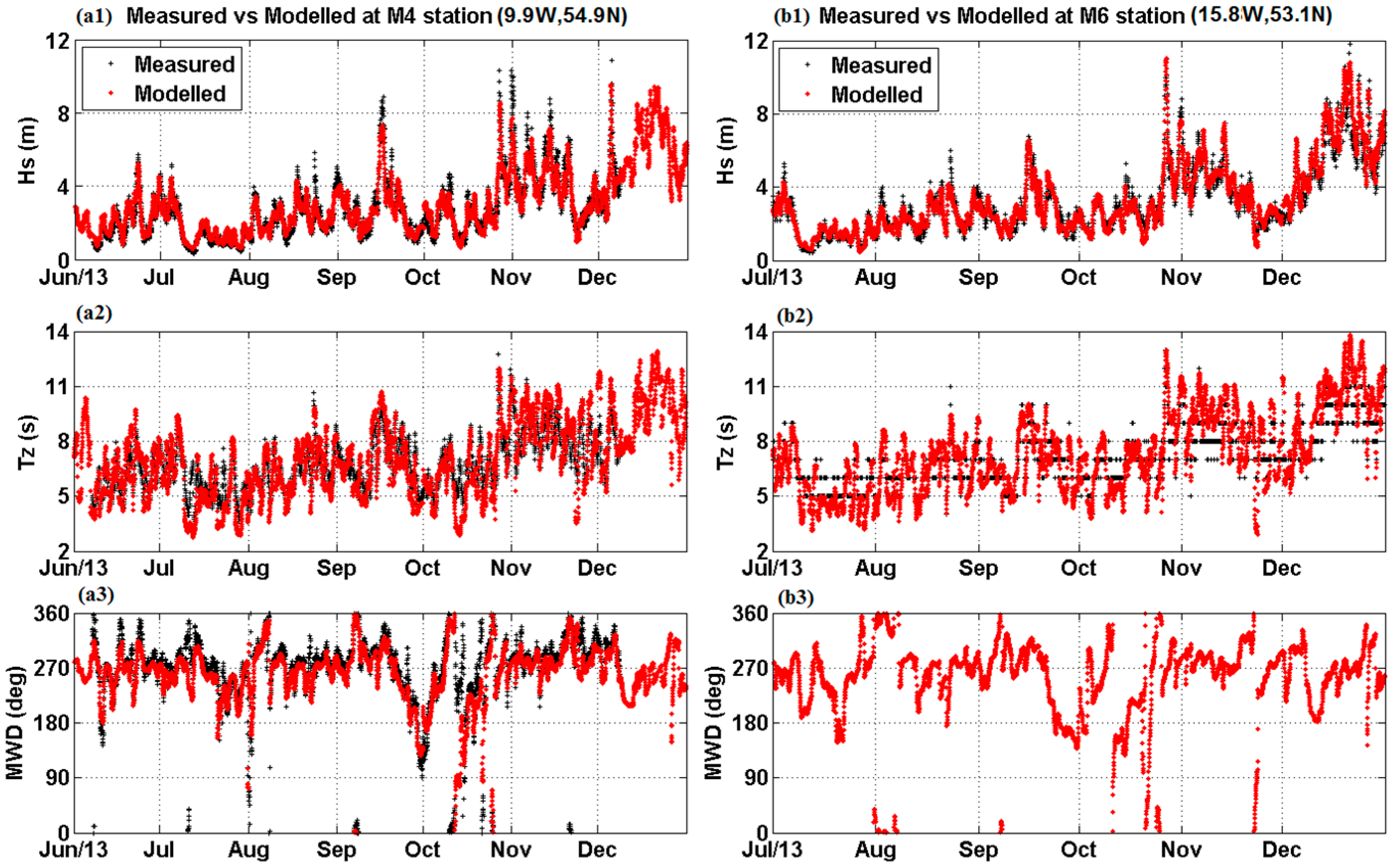
2.2. Coarse Ireland Model Development and Validation

The CI wave model has been developed with a spherical coordinates setup to reproduce the development of swell waves in large open waters including high wave events at regional scale before they reach Irish coastlines [26]. The CI model domain is illustrated in Figure 1a. The model resolution is 0.05° (gridded model) and covers a large area of the AO to the extent of 20 W to 3 W and 50 N to 59 N. The main wind forcing supplied as surface boundary conditions is taken from the European Centre for Medium-Range Weather Forecast (ECMWF) Era-interim [27] at 0.5° spatial resolution and 6 h time resolution. The wave data at the boundaries is extracted from a global WW3 wave model, developed by U.S. Navy Fleet Numerical Meteorology and Oceanography Centre (FNMOC) [28], at 6 h time intervals. The bathymetry data was retrieved from ETOPO1 at 1° spatial resolution [29]. Blue Kenue software (National Research Council Canada, Ottawa, ON, Canada) [30] was used to interpolate processed bathymetry datasets in order to generate the 0.05° resolution gridded model domain. Regarding model setup, the recommended geographical propagation for large geographical domains for non-stationary mode in SWAN is the Stelling and Leendertse (S&L) scheme. Early tests with the CI revealed that its performance was most sensitive to the type and parameterisation of the wave generation formulations. Model performance was assessed using the Komen [31], Yan [32] and Janssen [33] wave growth formulations [34] with the Komen formulation found to be most accurate. A series of calibration tests were then conducted to determine the optimum values for the dissipation coefficients, Cds and δ, in the Hasselmann white-capping formulation [35] which is used in conjunction with the Komen wave growth formula. The best model performance was achieved using dissipation coefficients of Cds = 3 × 10⁻⁵ and δ = 1.5. The CI wave model development, including sensitivity and calibration tests, is presented in detail in [36].
The modelled outputs were compared to available measured data [37] from wave buoys (see Table 1 and Figure 1a) located in Irish (BA, BB, M3, M4, M6) and Scottish (WH, BS) waters for calibration (November 2013) and validation (years 2008–2013) purposes. The wave buoys have good geographical spread throughout the CI domain and include deep, offshore waters and shallower, nearshore locations. A comparative statistical analysis between measured and modelled data for Hs, Tz and MWD was conducted for the 5-year validation period in order to determine model accuracy based on coefficient of determination (R2), root-mean square error (RMSE), bias and scatter index (SI) calculations.
A summary of validation values is tabulated in Table 2. The CI wave model managed to achieve equally high levels of accuracy for Hs at all locations; R2 ≥ 0.9 at all locations, RMSE ≤ 0.69 m at all location but one (WH) and bias within ±0.4 m at all locations. Accuracy for Tz was slightly less than for Hs, but still high, with R2 ≥ 0.77 at all locations. The accuracy of MWD was lower again but still acceptable; R2 was approximately 0.6 at all locations except at WH where it was just 0.4; however, WH is near the west coast of Scotland and is thus well outside the area of interest. Possible explanations for the poorer agreement in MWD than Hs and Tz are that wave buoys can cause greater directional spreading of the wave field in reality due to refraction [38] than might occur in the simulated wave fields and wave buoy directional properties often show erroneous behaviour below the peak frequency [39]. The accuracy of the CI model is further confirmed by the 2013 timeseries comparison of modelled and measured data at M4 and M6 shown in Figure 2.
The R2 values for Hs and Tz at the Irish offshore buoys (i.e., M3, M4 and M6 stations) are consistent with the published WW3 model validation values of 0.94 and 0.88, respectively, in [40]. Moreover, the RMSE and bias values of wave height were within the range (RMSE = 0.4–0.7 m, bias = 0.05–0.2 m) recommended by World Meteorological Organization (WMO) [41] for different parts of the world’s oceans. Thus, it is concluded that the CI wave model is capable of accurately reproducing wave conditions at oceanic and regional scales and is therefore suitable to provide nested boundary conditions for the high resolution AMETS wave model.
The CI model managed to achieve good accuracy in prediction of the wave conditions at BA and BB stations, especially at BA, which is in deep water. Accuracy was lower at BB; it recorded the lowest RMSE in Tz and highest bias in Hs across all the locations. The model’s poorer performance at BB is understandable as it is the location nearest the shore and therefore the one most susceptible to modelling inaccuracies resulting from the coarse spatial resolution. This demonstrates the need to develop a high resolution wave model at AMETS in order to avoid poor estimation of wave parameters for wave resource assessment.

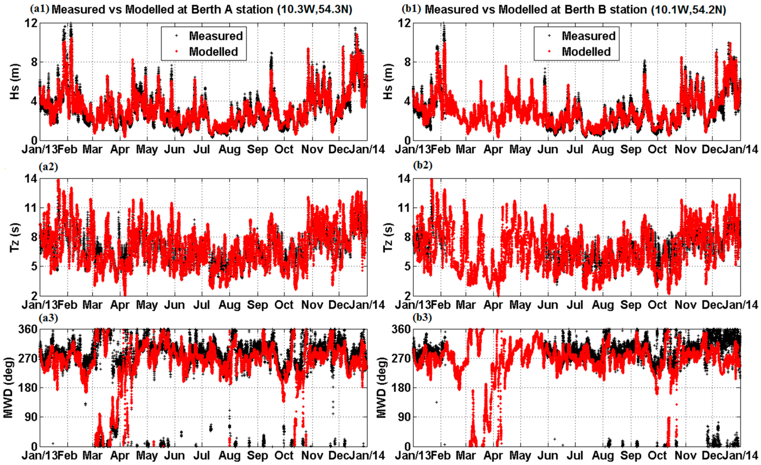
2.3. Atlantic Marine Energy Test Site Model Development and Validation

The high resolution AMETS wave model, resolved at 0.0027° resolution (approximately 300 m), has been developed to reproduce the development of wind-generated waves in limited local fetch including high wave events at local scale. Figure 1b shows the AMETS model domain, which covers 11.05 W to 9.7 W and 53.95 N to 54.65 N. The bathymetry data was obtained from INFOMAR datasets at 250 m resolution [42] and the Blue Kenue software was used to interpolate processed bathymetry datasets in order to generate the 300 m resolution gridded model domain. High resolution wind data from ECMWF at 0.125° spatial resolution and 6 h time resolution were used as surface boundary conditions, while the open boundary conditions were supplied from the nested spectral boundary outputs generated by the CI wave model at 30 min intervals. The orientation of the model is 0° clockwise in a spherical geometrical coordinate system to ensure all open boundaries are close to 90° for all major in- or outflow wave formations. Initially, the CI model setup was adopted for the AMETS model. While its performance was quite good, further calibration runs for different values of Cds and δ were conducted for a month period (December 2013). The best AMETS model performance was achieved for Cds = 2 × 10⁻⁵ and δ = 2. This setup achieved the same R2 and RMSE values as the CI model setup but produced lower bias values especially for Tz (0.8 s at BA and 0.3 s at BB compared to 1.1 s and 0.5 s respectively, for the CI setup). More details of the AMETS calibration tests are presented in [43]. Similar to the CI model, the performance of the AMETS model was assessed based on model validation parameters of R2, RMSE, Bias and SI for Hs, Tz and MWD. Table 3 shows the validation values of model performance at BA (2012–2013) and BB (2010–2013). For Hs, the model achieved R2 = 0.95 at both stations, RMSE values were below 0.6 m and bias values were less than 0.2 m. For Tz, R2 values were ≥0.8, RMSE were ≤1.4 s and bias values were less than 0.2 s at BA and close to 0 at BB. Finally for MWD, R2 were ≥0.64, RMSE were ≤27° and bias were ≤9°. The performance statistics indicate an acceptably high level of model accuracy which is also demonstrated visually by the timeseries comparison of modelled and measured data in Figure 3. It was therefore concluded that the AMETS wave model managed to satisfactorily replicate wave conditions at a local scale and was sufficient to be used in a detailed wave assessment analysis of the AMETS berths.
Comparing the validation values of the AMETS model at BA and BB with those of the CI model, it is seen that model accuracy is indeed improved by the higher resolution, particularly at the nearshore BB. For Hs, R2 was increased from 0.92 to 0.95, RMSE was reduced from 0.69 to 0.52 m and bias was improved from −0.4 to 0.17 m. Similarly, for Tz, R2 was increased from 0.77 to 0.8, RMSE was reduced from 1.74 to 1.4 s and bias was reduced from 0.23 to 0.01 s, and for MWD, R2 was increased from 0.57 to 0.64. The validation values at BB were also compared with those from other published wave model studies of Irish waters including those of [12,44] using SWAN and of [40] using WW3 (see Table 3). It is observed that the authors AMETS model achieved better accuracy than the models of [12,44], particularly with respect to Tz predictions. Our AMETS model achieved a similar level of accuracy to the WW3 model of [40] for Hs and although [40] achieved slightly higher R2 and lower RMSE for Tz, our model achieved almost zero bias while the bias of [40] was 0.65 s. All of these comparisons provide further confidence in the accuracy of the AMETS model.

3. Resource Assessment Results

Wave height (Hs), wave energy period (TE) and wave power (P) are all important design parameters for wave energy device survivability and energy extraction, thus, each parameter was assessed individually at both BA and BB. Each assessment involved three stages:
(1)
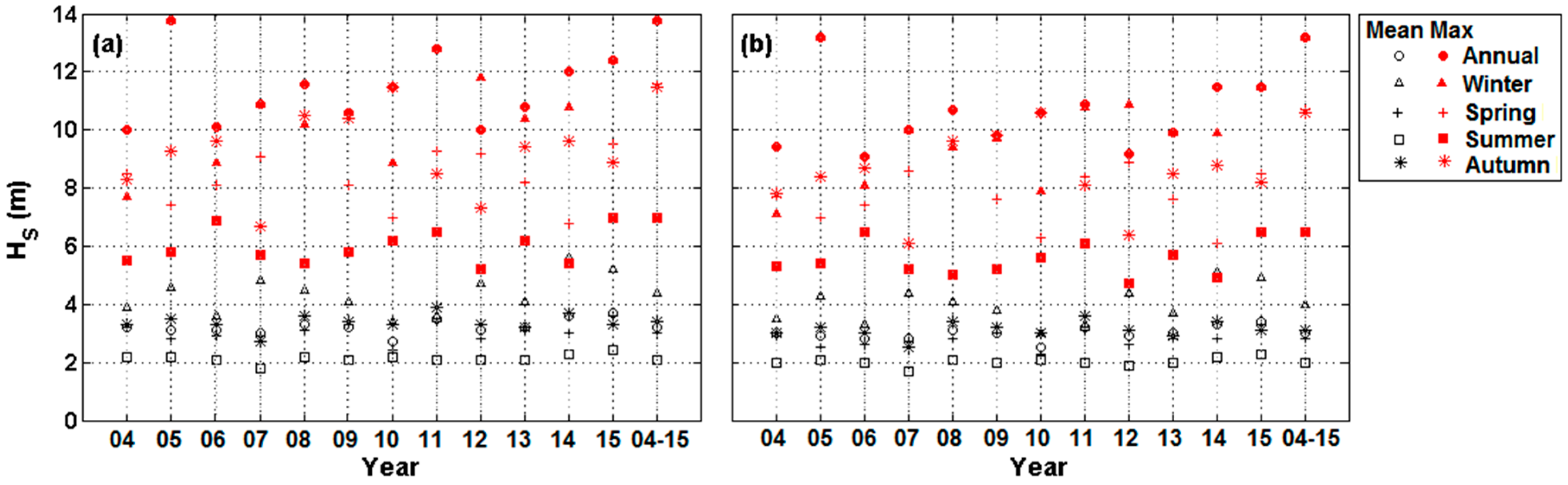
Assessment of mean conditions;
(2)
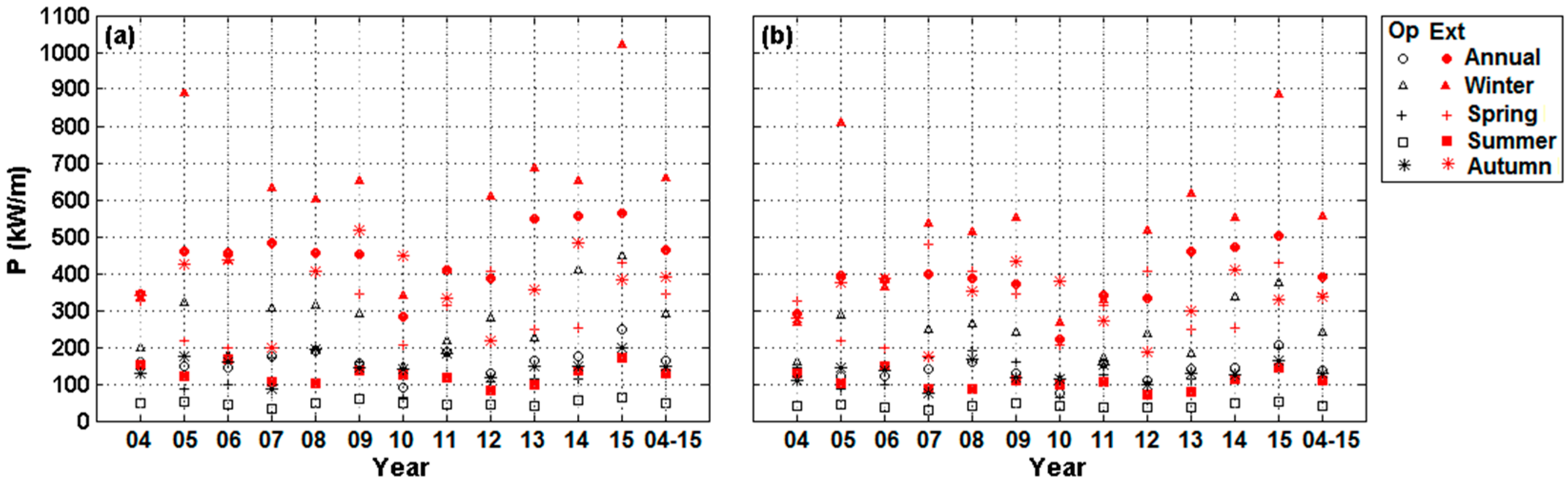
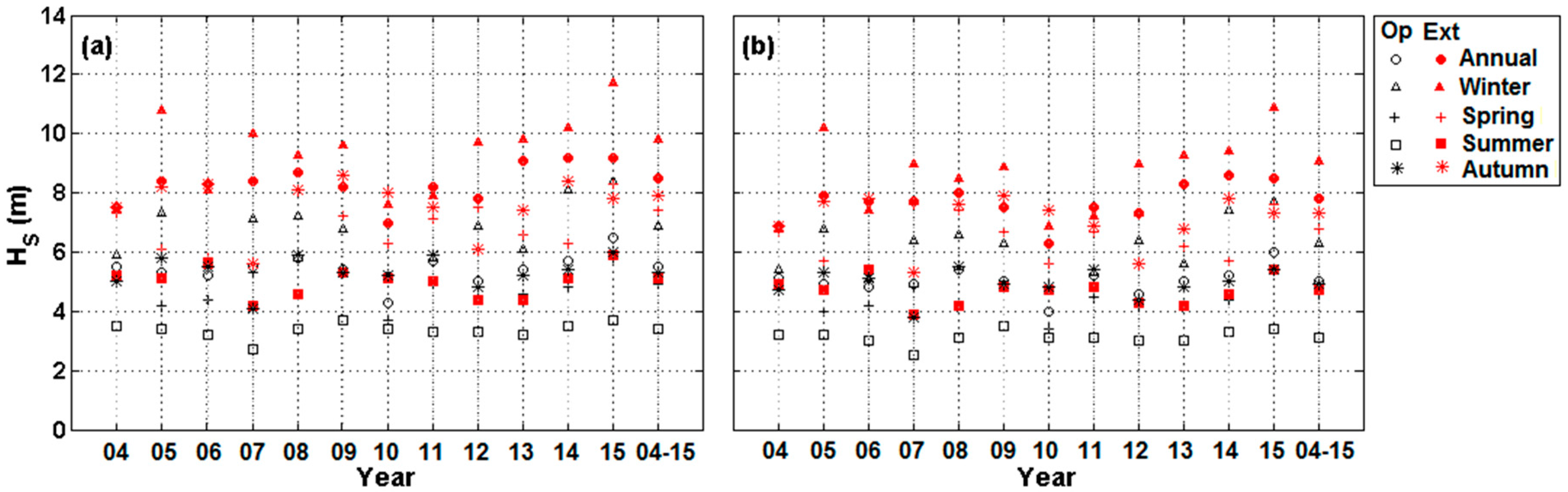
Characterisation of operational, high and extreme conditions;
(3)
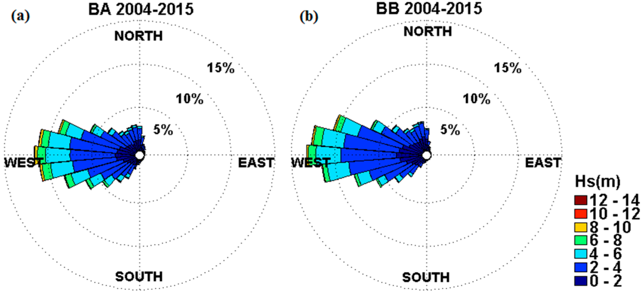
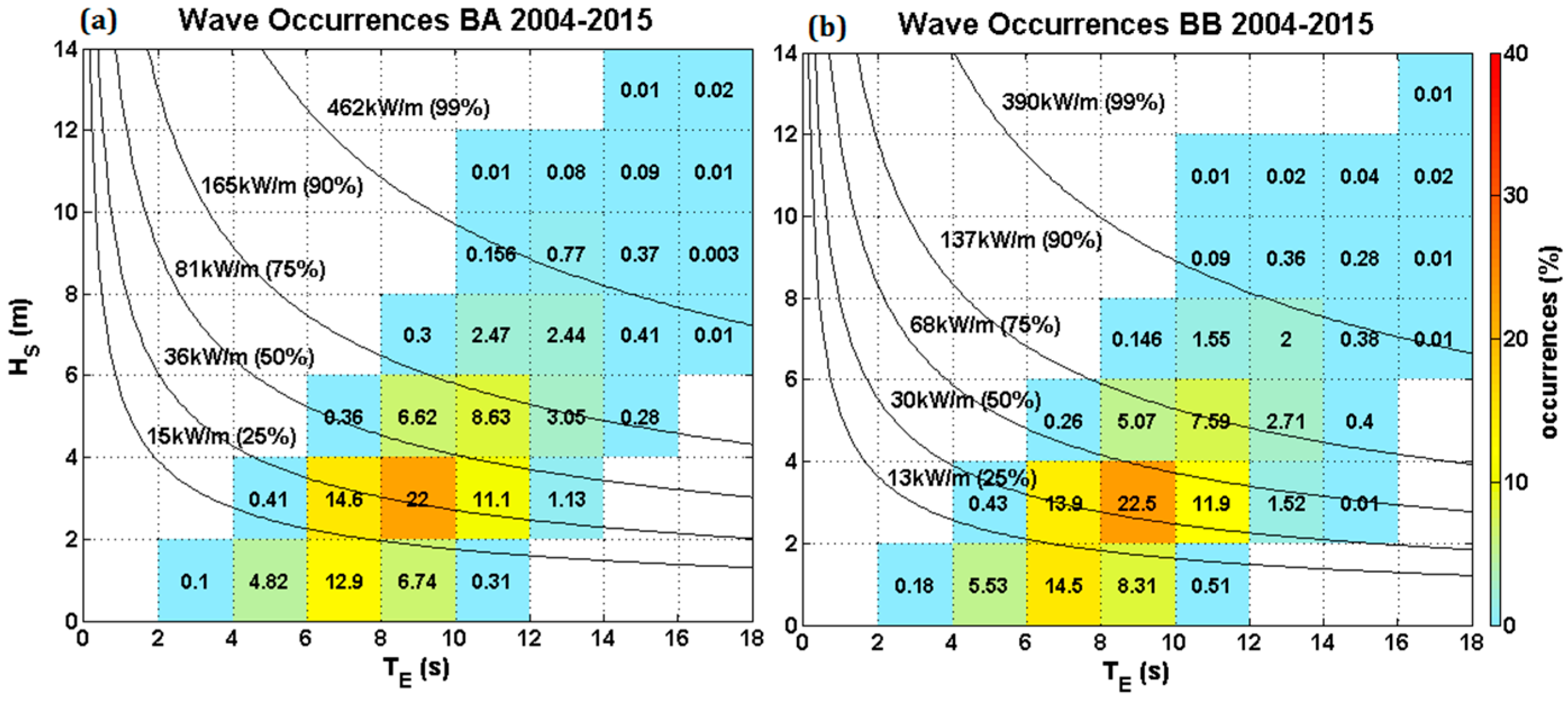
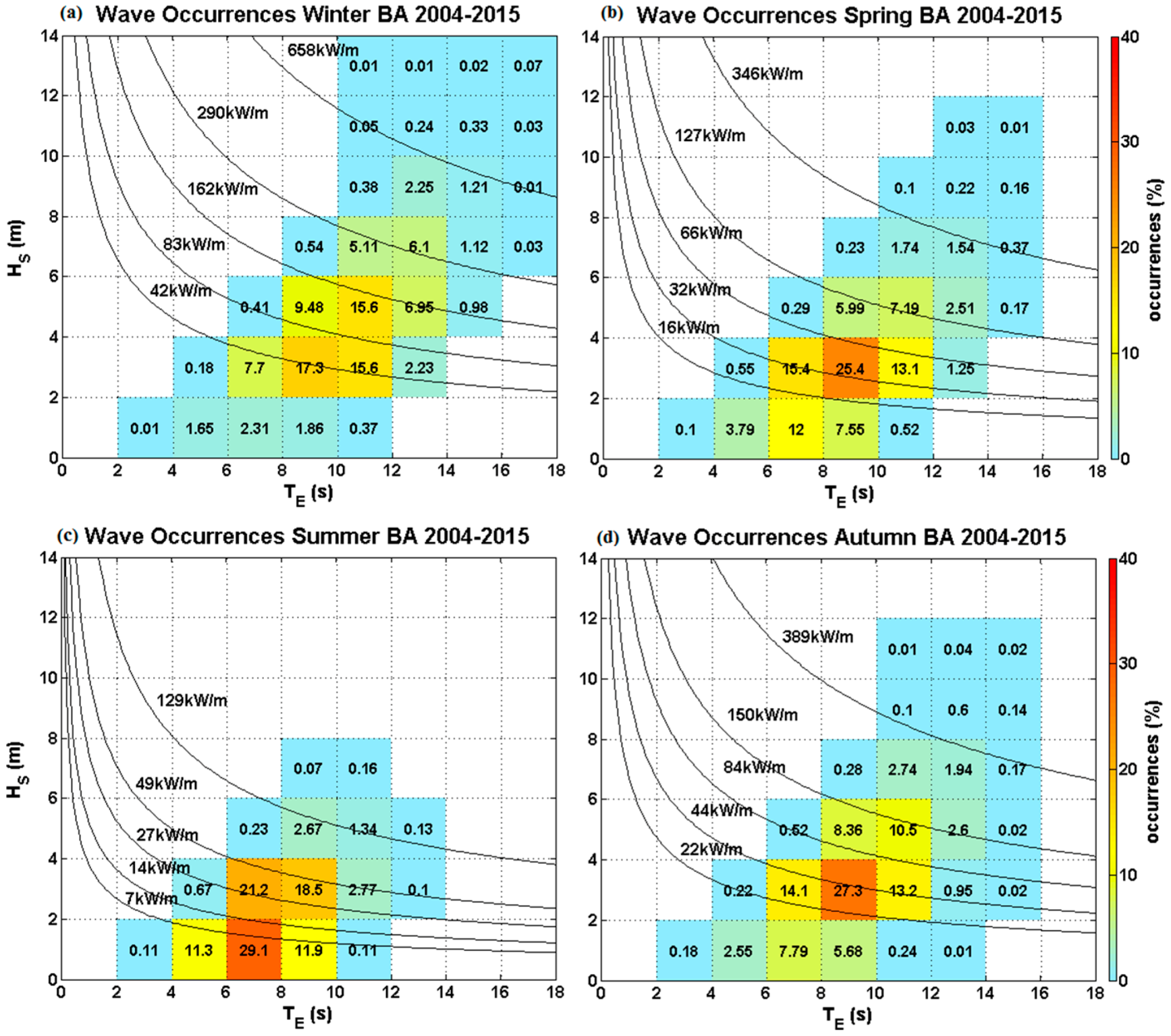
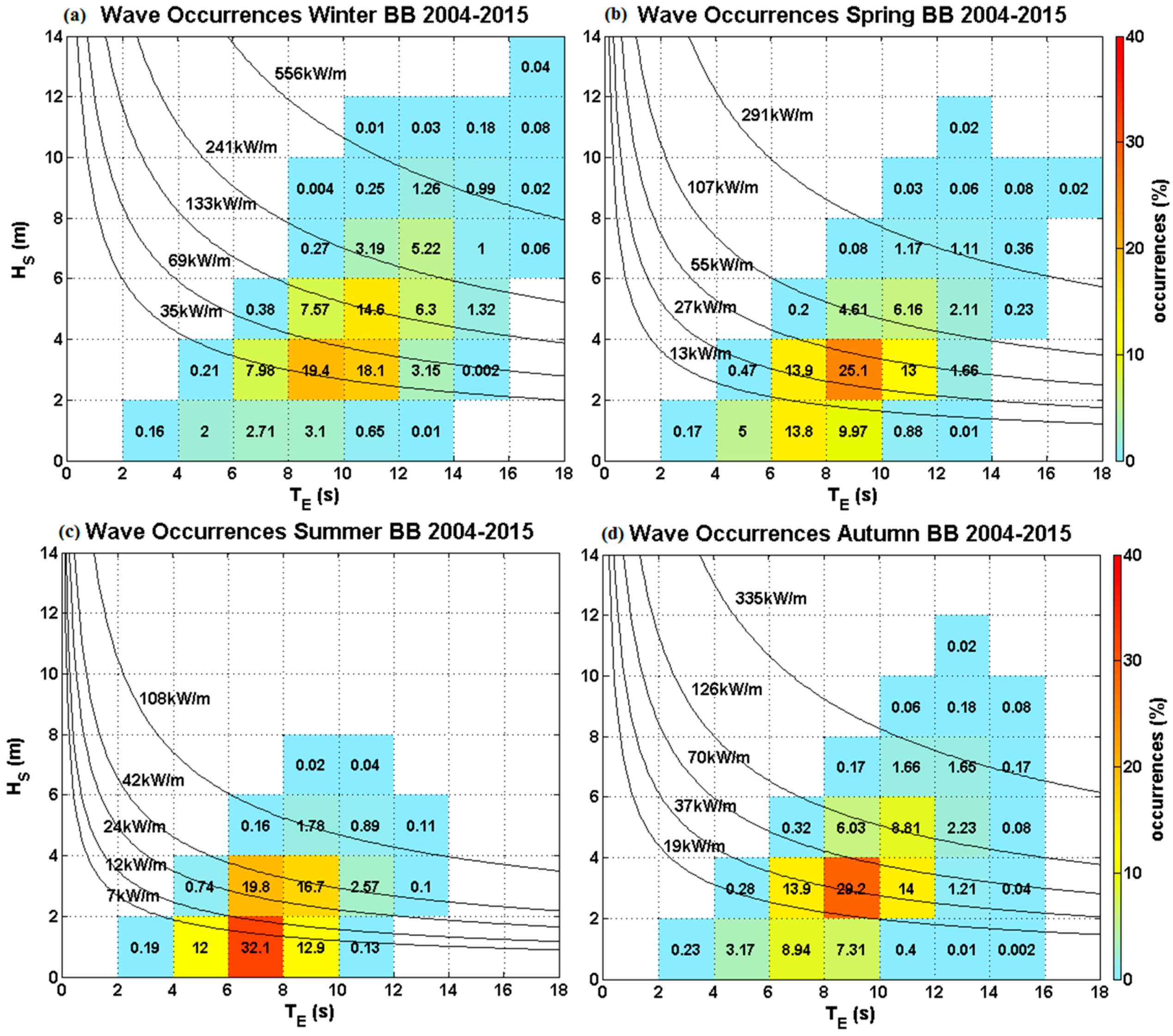
Joint occurrence analyses—with MWD in the cases of Hs and TE and between Hs and TE in the case of P.
The assessments were based on 12-years of data from January 2004 to December 2015 output from the high resolution AMETS model at 30 min intervals. Some contour maps are also presented for the large CI model domain based on CI model data output at 1 h intervals. Values for Hs, TE, MWD and wavelength (λ) were output directly from the model.
Local water depth dictates how one should calculate wave power. According to linear wave theory [45], deep water conditions exist where d/λ > 1/2 (d = water depth and λ = wave length) while transitional water conditions exist where 1/2 > d/λ > 1/20. For deep water, the wave power (P) per unit width of wave crest (kW/m) of a regular sea state can be calculated using [46]:
P = 0.49 H s 2 T E
while for transitional water, P can be calculated using:
P = 0.63 H s 2 C g
where Cg is wave group velocity. Table 4 presents values of d/λ calculated at BA and BB for 12-year mean annual and seasonal wavelengths and shows that d/λ > 1/2 persists for all cases; thus both sites are considered deep water and Equation (2) is used to calculate the available wave power.
Stages (1) and (2) of the assessment include annual and seasonal analyses which are based on the following time periods:
Annual period: January to December of current year;
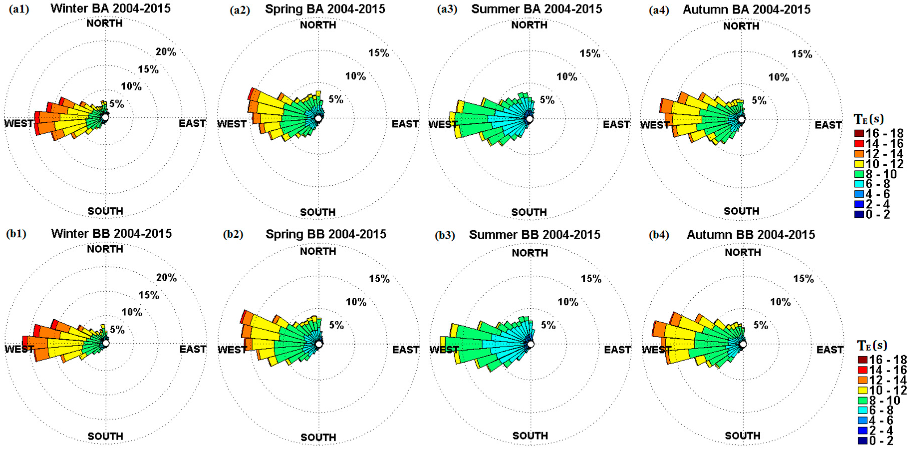
Winter period: December of previous year, January and February of current year;
Spring period: March, April and May of current year;
Summer period: June, July and August of current year;
Autumn period: September, October and November of current year.
It should be noted that the winter period for a particular year runs from December of the previous year to February of the current year, while the annual period runs from January to December of the current year. Hence, some small discrepancies may exist between the yearly and seasonal analyses results. In addition, boundary conditions for December 2003 were not available from FNMOC, thus, winter 2004 was analysed from January to February 2004 only.
The approach used to characterise wave conditions considers percentage of occurrences of wave conditions and uses criteria for operational, high and extreme events defined as percentiles of normalised wave parameter data. Figure 4 shows a graphical representation of the characterisation methodology which is described in more detail in [47]. The characterisation of a site by wave parameter, γ, is conducted simply by graphing the normalised wave parameter data (Figure 4b) and applying the following criteria:
Operational events: events falling between 0th and 90th percentiles;
High events: events falling between 90th and 99th percentiles;
Extreme events: events falling between 99th and 100th percentiles.
Identifying the operational wave conditions at a wave energy site is important as a wave energy device should be designed to extract power most efficiently in those conditions given that they will occur most often. On the other hand, knowledge of the extreme conditions at a site is extremely important for device survivability design.

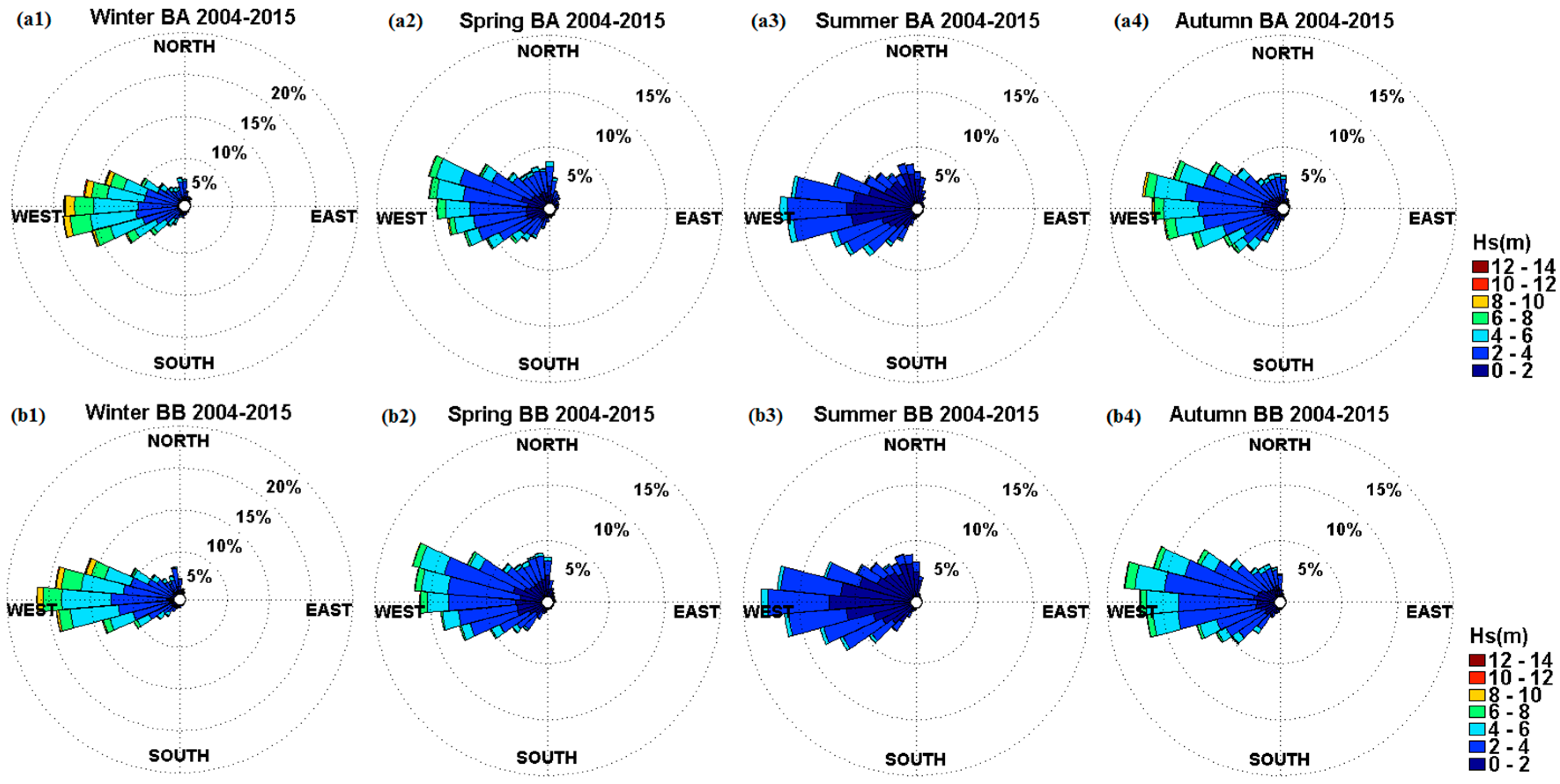
3.1. Significant Wave Height

Contour maps of the 12-year annual means of Hs (and MWD) from the regional-scale CI model and the local-scale AMETS model are shown in Figure 5. Figure 6 shows similar maps of the 12-year seasonal means. As would be expected, Figure 6 shows that Hs values gradually decrease as one moves from the deeper waters of the AO towards the Irish west coast. Annual means off the Irish west coast are approximately 3.5 m but fall to approximately 3 m at AMETS. In offshore areas, the dominant 12-year mean MWDs are from the southwest but are more westerly in near-shore areas. Figure 6 shows there is significant seasonal variation in Hs in both offshore and nearshore areas but little seasonal variation in MWD with the 12-year MWDs being primarily from the west.
Summaries of the annual and seasonal mean Hs values at BA and BB are shown in Figure 7a,b, respectively. Instantaneous maximums are also included in the figures (plotted values and standard deviations are given in Table A1 and Table A2 in Appendix A. Hs trends are quite similar at both berths but with slightly higher values calculated at BA; this is understandable given the proximity of the berths and the greater water depth at BA (100 m compared to 50 m at BB). Mean annual Hs were 3.2 m and 3.0 m at BA and BB, respectively. The annual mean Hs values at BA varied between 2.7 and 3.7 m while at BB the values ranged from 2.5 to 3.4 m. These annual means are consistent with the annual mean Hs values of 2.5–3.5 m published in [7] for the west coast of Ireland. Although there is some variation in annual means, inter-annual variation is most significant for the winter period with winter means at BA, for example, ranging from 3.4 to 5.6 m. By comparison, summer means at BA only varied from 1.8 to 2.4 m. Inter-seasonal variation in Hs is significant with highest waves occurring in winter and lowest waves occurring in summer; autumn waves are typically slightly higher than spring. There was approximately 2 m difference in the 12-year winter and summer means, but the winter-summer difference was greater than 3 m in 2007 and 2014. 2010 and 2014 were notable years for having the lowest and highest annual and winter means of the 12 year period. The maximum instantaneous Hs values of 13.8 m at BA and 13.2 m at BB were recorded in winter 2005.
A detailed summary of the operational and extreme Hs characterisation thresholds at BA and BB is presented in Figure 8a,b, respectively (plotted values are given in Table A3 and Table A4 in Appendix A). Operational events are those below the operational threshold while extreme events are those above the extreme threshold and high events are those falling between the two thresholds. Looking first at the characterisations for the full 12-year period, the operational Hs thresholds were 5.5 m at BA and 5.0 m at BB, while the extreme Hs thresholds were 8.5 m at BA and 7.8 m at BB. Annually, the operational threshold ranged from 4.3 to 6.5 m at BA and from 4 to 6 m at BB, while the extreme threshold ranged from 7.0 to 9.2 m at BA and from 6.3 to 8.6 m at BB. 2010 recorded the lowest annual operational and extreme thresholds and 2015 gave the highest. For example, at BA the operational threshold was 4.3 m in 2010 compared to 6.5 m in 2015. Looking next at the seasonal characterisation thresholds, the inter-seasonal variation in wave conditions is evident with winter thresholds being significantly higher than summer thresholds. At BA, for example, winter and summer operational thresholds were 6.9 m and 3.4 m, respectively, and winter and summer extreme thresholds were 9.8 m and 5.1 m, respectively. Operational and extreme thresholds in autumn are typically higher than those in spring.
Wave direction is also an important parameter to be considered in WEC design, especially for terminator- and attenuator-type devices where performance is sensitive to the angle of the device relative to the wave direction, and for determining optimum layouts of WEC arrays [48]. Joint occurrence of Hs and MWD was investigated using wave rose plots. Figure 9 shows the wave rose plots for BA and BB based on the full 12-year dataset while Figure 10 shows 12-year seasonal wave rose plots at both locations. Based on the data in Figure 9, it was found that the dominant MWDs for operational Hs at BA and BB were south-west, west and north-west while for extreme Hs events the dominant MWDs were mostly northwest. A similar trend in MWD was also noted from the 12-year seasonal wave plots and also that there is a slight shift from west to northwest dominance in the spring and autumn periods.

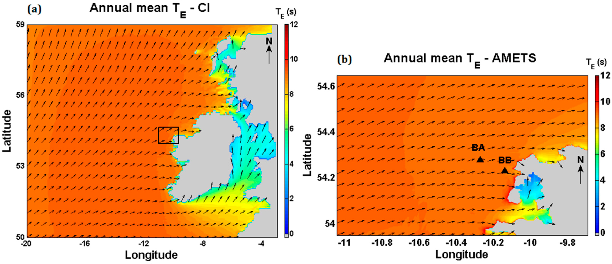
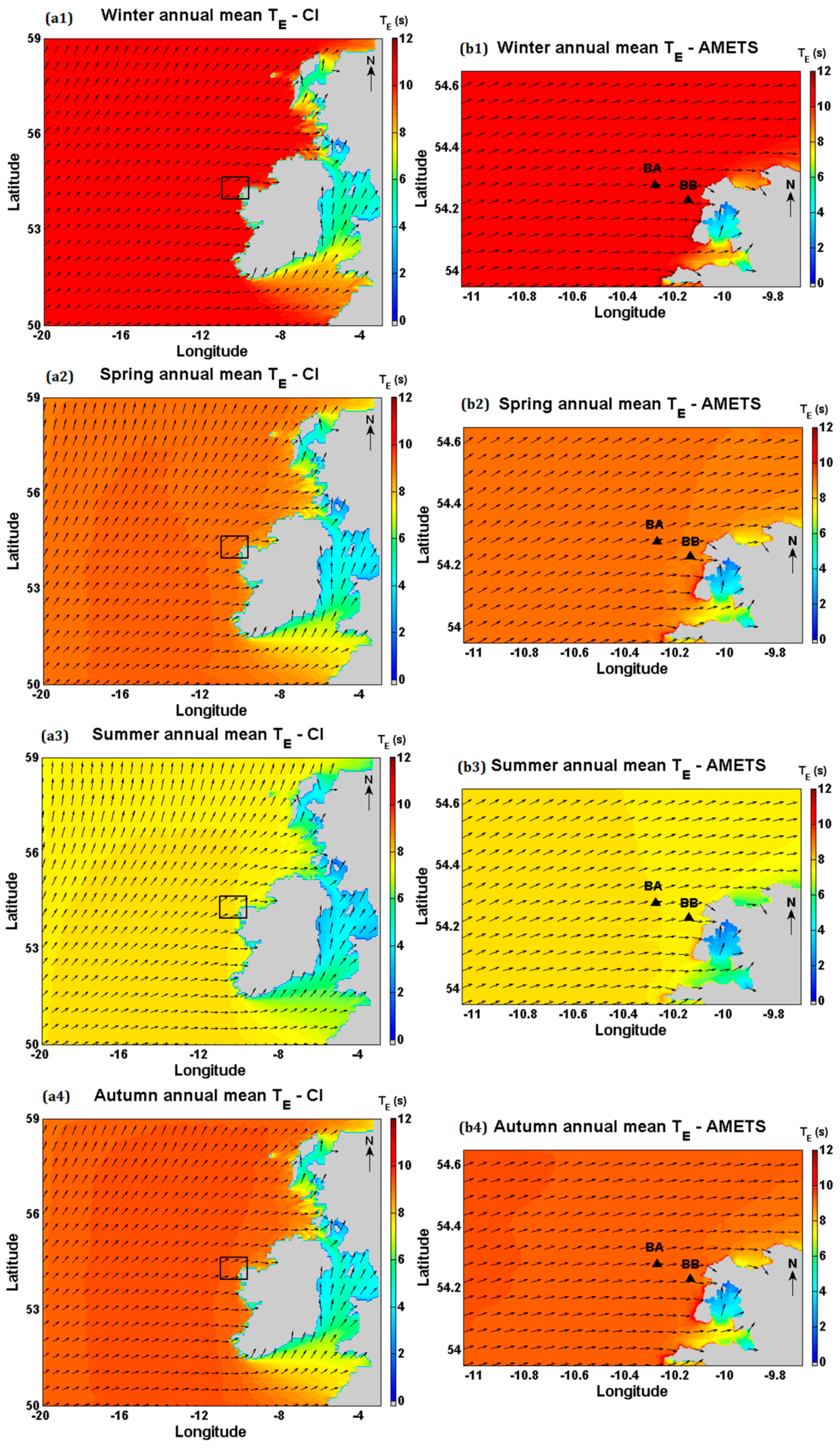
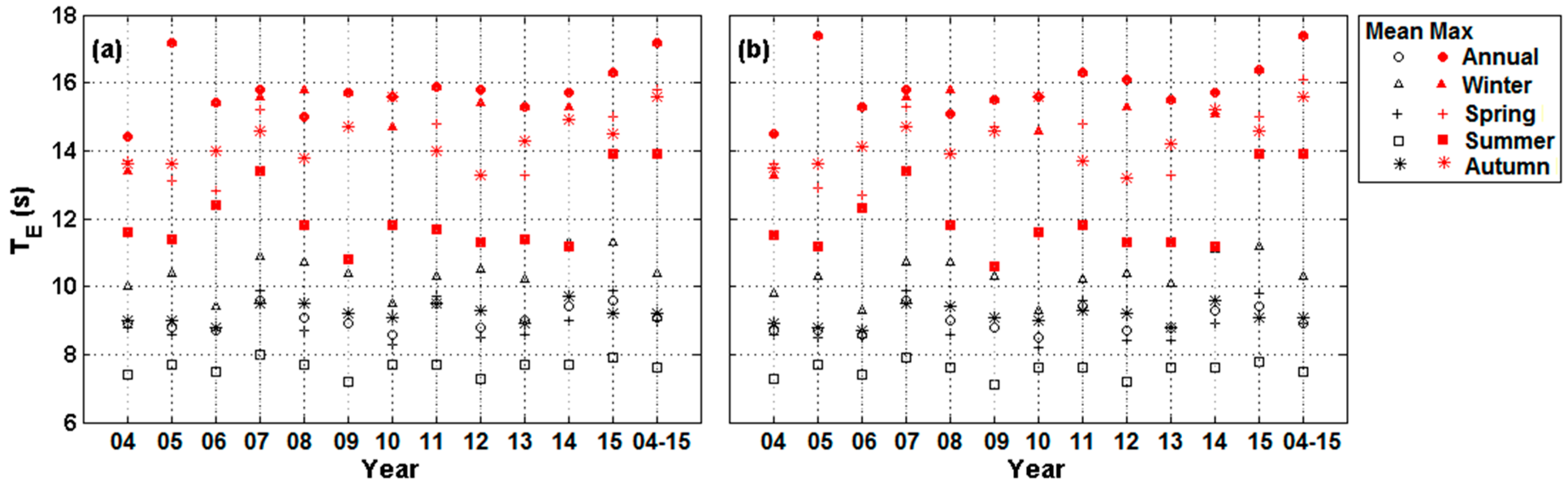
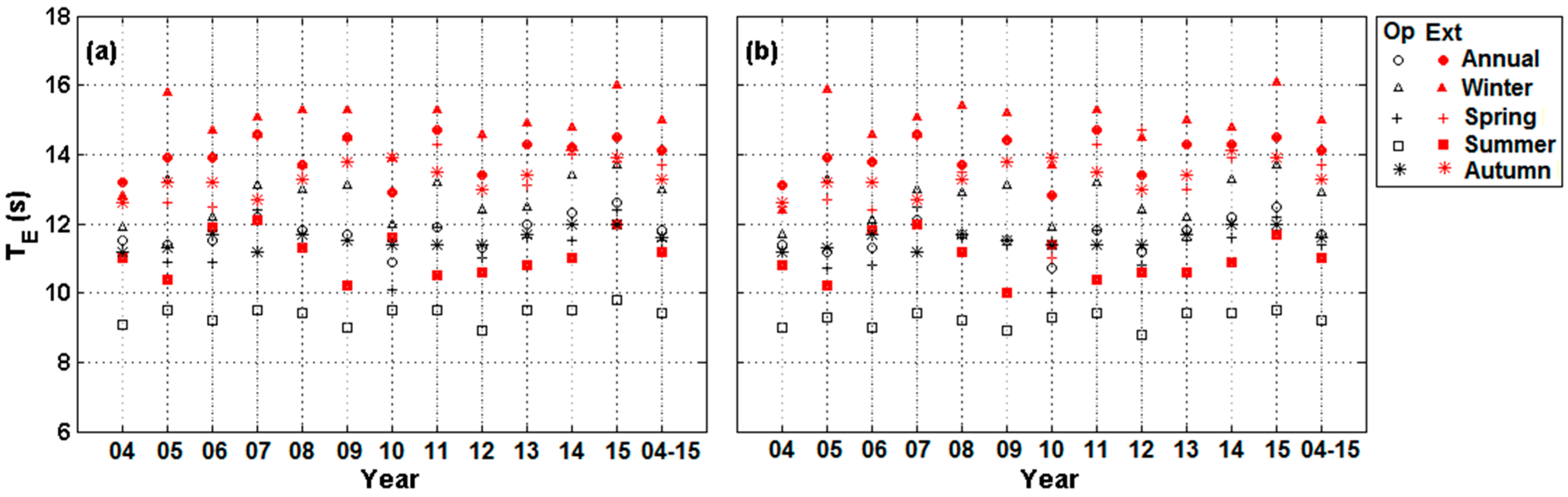
3.2. Energy Wave Period
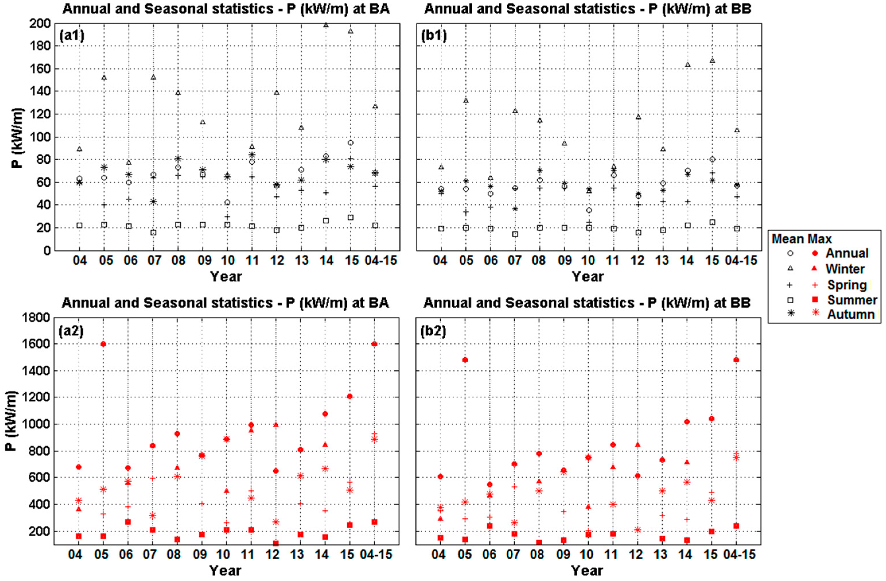
Figure 11 and Figure 12 show contour maps of the 12-year annual and seasonal means of TE (and MWD) from the CI and AMETS models. Generally, the deep water areas show longer mean wave periods than shallower waters but the spatial change is TE is relatively small until one enters the extreme near-shore area. The 12-year mean TE near AMETS is approximately 9 s which is similar to that much further offshore in the AO. Similar to wave heights, significant inter-seasonal variation in wave period is observed from Figure 12 with mean winter energy wave periods in the region of 10–11 s compared to mean summer periods of 7–8 s.
A detailed summary of annual and seasonal mean TE values are presented in Figure 13a,b for BA and BB, respectively (see detailed values in Table A5 and Table A6 in Appendix A). The maximum wave periods recorded for the particular periods are also given. As for wave heights, the proximity of the berths means that mean wave periods are quite similar at both sites, the 12-year annual mean at BA being 9.1 s compared to 8.9 s at BB, for example. The slightly higher TE values at BA are a result of the deeper water at that berth. Inter-annual variation is evident with annual means ranging from 8.5 to 9.6 s at both berths and similar to wave height, inter-annual variation is more significant in winter than in summer. Inter-seasonal variation in TE is also evident with 12-year mean winter and summer periods of 10.4 s versus 7.6 s at BA and 10.3 s versus 7.5 s at BB. As for wave height, 2010 and 2015 were again notable as the years with the lowest and highest annual mean TE and 2005 also yielded the maximum TE values recorded during the 12-year period, these being 17.2 s and 17.4 s at BA and BB, respectively.
Figure 14a,b presents the annual and seasonal energy wave period characterisation thresholds at BA and BB, respectively (see detailed values in Table A7 and Table A8 in Appendix A). The operational TE thresholds for the 12-year period were 11.8 s at BA and 11.7 s at BB, while the 12-year extreme TE threshold was 14.1s at both locations. Annually, the operational TE thresholds at BA varied from 10.9 to 12.6 s and at BB they varied from 10.7 to 12.5 s. The annual extreme TE thresholds varied from 12.8 to 14.7 s at both sites. 2010 and 2015 again yielded the lowest and highest annual threshold values, respectively. Looking at seasonal characterisation, the operational and extreme TE thresholds are highest in winter and lowest in summer and the inter-annual variation in threshold values is greatest in winter and smallest in summer. For operational thresholds, for example, the 12-year winter value was 13 s at both berths compared to 9.4 s (BA) and 9.2 s (BB) for the summer, while for extreme thresholds, the 12-year winter value was 15 s at both berths compared to 11.2 s (BA) and 11 s (BB) for the summer. Annually, autumn operational TE thresholds are typically slightly higher than those for spring while the opposite is true for extreme TE thresholds.
As for Hs, the joint occurrence of TE and MWD was also investigated. Figure 15 shows wave rose plots for BA and BB based on the full 12-year period while Figure 16 shows 12-year seasonal wave rose plots.

3.3. Wave Power

Figure 17 and Figure 18 show contour maps of the 12-year annual and seasonal means of available wave power, P, calculated using Hs and TE values from the CI and AMETS models. It can be seen that the wave power resource off Ireland’s west coast is indeed significant with annual mean powers in the range of 80–90 kW/m available in the Atlantic Ocean. Wave power dissipates quite rapidly near the coast, as waves lose energy due to friction effects in the shallower water depths. This can be clearly seen in the AMETS model maps where annual mean P at BA is approximately 70 kW/m and drops to about 60 kW/m at BB which is just 10 km away. Figure 18 shows that there is significant seasonal variation in the wave power resource with winter levels being five times greater than summer levels (e.g., 110–120 kW/m versus 20–25 kW/m for the Atlantic Ocean).
Figure 19 contains summaries of the annual and seasonal mean and maximum P calculated at BA and BB, respectively (see detailed values in Table A9 and Table A10 in Appendix A). The 12-year mean annual wave powers were 68 kW/m at BA and 57 kW/m at BB. These differ with the annual mean P of 77 kW/m and 62 kW/m calculated at BA and BB, respectively, by [12]; this is likely due to the higher accuracy achieved by the present model. Our annual mean P estimates are consistent with other published estimates for the area, e.g., [49] reported annual mean P of 69 kW/m at BA and 59 kW/m at BB and [6] report an annual mean P of 70 kW/m in the region around BA.
There is significant inter-annual variability in mean P at both berths, annual means ranged from 42 to 95 kW/m at BA and 35–80 kW/m at BB. As would be expected from the trends in Hs and TE, 2015 was the most energetic year with the highest annual mean P while 2010 was the least energetic. Again following the trends in Hs and TE, power availability is highest in winter and lowest in summer (12-year means were 127 kW/m versus 22 kW/m at BA and 106 kW/m versus 19 kW/m at BB) and power availability in autumn is typically higher than in spring. 2005 saw the maximum instantaneous power levels at the sites during the 12 year period with 1599 kW/m and 1480 kW/m computed at BA and BB, respectively.
Looking at the spatial variation in resource between the berths, the seasonally-averaged power levels at BB are approximately 15% lower than those at BA; this is likely due to the more shoreward location of BB and its shallower water depth relative to BA.
The operational and extreme thresholds determined for BA and BB are presented in Figure 20a,b, respectively (see detailed values in Table A11 and Table A12 in Appendix A). The 12-year operational P thresholds were 165 kW/m at BA and 137 kW/m at BB and ranged annually from 90 to 250 kW/m and 74–207 kW/m, respectively. The 12-year extreme P thresholds were 462 kW/m at BA and 390 kW/m at BB and varied annually from 282 to 565 kW/m and 222–503 kW/m, respectively. At BA, winter operational thresholds ranged from 148 to 448 kW/m compared to a summer range of 32–62 kW/m while at BB, winter operational thresholds ranged from 112 to 375 kW/m compared to the summer range of 28–51 kW/m.
A joint occurrence analysis between Hs and TE was conducted for the 12-year set of P data at BA and BB (Figure 21). The wave power characterisation thresholds are included by overlaying the 90th (operational threshold) and 99th (extreme event threshold) wave power percentile isolines on the bi-variate scatter plots. The 25th, 50th and 75th percentile lines are also included for additional information. These plots give a very useful indication of the ranges of Hs and TE of the waves that comprise operational and extreme wave power events; such information should be of significant interest to WEC developers interested in testing devices at AMETS. It is observed that the most common operational P conditions comprise waves with Hs between 0 and 4 m and TE between 6 and 12 s; such waves account for more than 60% of the wave conditions at both stations. Extreme P conditions typically comprise waves with Hs between 7 and 14 m and TE between 10 and 18 s. Figure 22 and Figure 23 show bivariate scatter plots of Hs versus TE for 12-year winter, spring, summer and autumn periods at BA and BB, respectively. The seasonal variation in sea conditions and available wave power is again easily observed.

4. Discussion

The assessment results above provide a comprehensive statistical description of the wave resource at the AMETS test berths which should be a useful asset to wave device developers interested in testing their devices at the full-scale test site. Traditional resource assessments tend to focus on available wave power only. While available power data is of significant interest to device developers with regard to estimating power outputs, the present assessment also includes independent assessments of wave height and wave period. The operational event thresholds identified for wave height and period could be used to help tune device performance to the ranges of conditions that occur most often at the berths, while the extreme event thresholds for Hs can be used to inform survivability design; for example, they could be used to estimate impact loads or to trigger the entrance of a device into survivability mode. By providing seasonal analyses, device developer can optimise the setups of their devices to perform best at the time of year that deployment at the site is likely to take place.

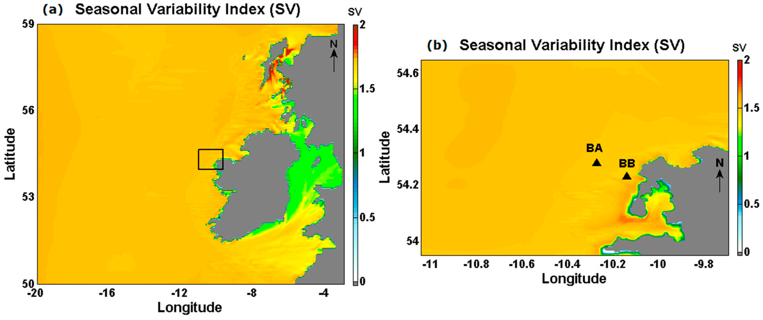
4.1. Resource Variability

One of the most important results of the resource assessment is the variability in wave height, period and power at the site. As seen in Figure 24a, the seasonal variability is well defined and very significant. Winter provides the most powerful waves and summer the least; on average, summer power levels are 80% less than winter levels. Autumn and spring periods provide similar levels of power which are, on average, approximately 50% of winter levels.
Figure 25a plots the annual mean powers for the 12-year period at the two berths and shows that inter-annual variations in the resource are also significant with the annual means in the least energetic year (2010) being approximately 60% lower than those in the most energetic year (2015). The scale of the annual variations highlights the importance of using long-term data sets (10 years minimum) for wave resource assessments. For example, a previously published wave resource assessment of AMETS [50] was based on measured waverider data from 2010 alone and it therefore under-estimates the conditions at the site given that 2010 was a particularly low energy year.
Additional analysis of variability was conducted by calculating the seasonal and monthly variability indices (SV and MV, respectively) proposed by [46] as:
S V = P s 1 P s 2 P y r
M V = P m 1 P m 2 P y r
where Ps1 and Pm1 are the mean P for the most energetic season and month, respectively, Ps2 and Pm2 are the mean P for the least energetic season and month, respectively, and Pyr is the mean annual P. Index values greater than 1 indicate significant variability. Figure 26a,b shows the distribution of 12-year SV across the CI and AMETS model domains while Figure 27a,b shows the 12-year MV distribution. There is a noticeable difference in variability in the Atlantic Ocean to the west of Ireland compared to the Irish Sea to the east with the more sheltered Irish Sea showing less variability. SV values at BA and BB are 1.51 and 1.49, respectively; meaning the normal range in available power between winter and summer is approximately 1.5 times the annual mean power. Monthly variability is even more significant at the test berths with MV values of 1.87 and 1.84 at BA and BB, respectively.
Looking further at the inter-annual variations in seasonal mean powers at BA (Figure 24b), it is seen that the majority of the variability occurs during the winter period where the difference between the highest and lowest powers was 132 kW/m. In contrast, there is very little variation in summer with the difference between the highest and lowest powers being just 13 kW/m. The North Atlantic Oscillation (NAO) is a significant driver of climate variability, particularly in winter, in northwest Europe. It is measured using the NAO index and it has been shown [51] that a strongly positive NAO results in a winter with strong north Atlantic westerlies while a strongly negative NAO results in a winter with weaker Atlantic winds. Studies of the wave energy resource in the waters off western coast of UK [52,53] have shown there is a correlation between inter-annual variability in winter wave power and the NAO index. This relationship was explored for the AMETS site by averaging the monthly NAO index values [54] during winter (December–January–February) to give annual mean winter NAO indices and conducting a regression analysis against annual mean winter powers at BA. Figure 25b shows there is a significant (R2 = 0.65) and positive relationship between the two variables with strongly positive winter NAO indices corresponding to high power levels (>180 kW/m) and strongly negative NAO indices corresponding to relatively low power levels (<70 kW/m). This finding is significant for future wave resource studies off the west coast of Ireland where only short-period datasets are available; by inspecting the corresponding winter NAO indices one could make some inference as to whether the assessment might be under- or over-estimating the mean resource.

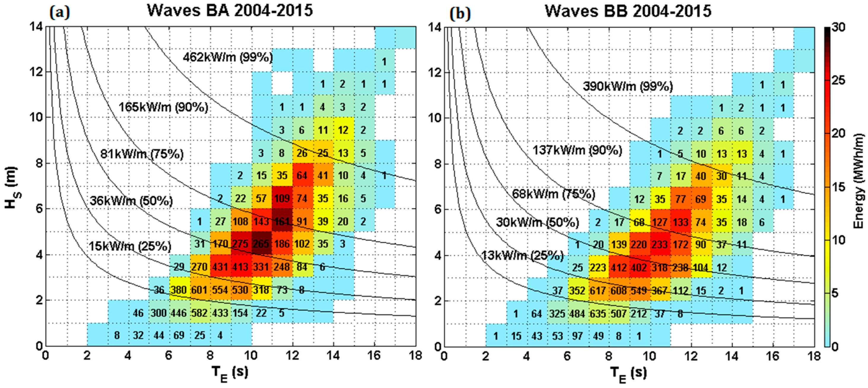
4.2. Energy versus Power

The bi-variate scatter plots of Hs-TE in Figure 21 show the sea states that occur most frequently are those where Hs ranges between 2 and 4 m and TE ranges between 8 and 10 s. For these sea states, the available power ranges from 15 to 80 kW/m. Higher levels of wave power are available but they occur less frequently; however, it may be possible to capture more energy at these times. Figure 28 shows two more bi-variate scatter plots of Hs versus TE which this time show the contribution of sea states to total annual energy. It can be seen that the most frequently occurring sea states do not contribute the most energy; rather there is an upward shift in the most significant sea states with most energy being generated by sea states where Hs ranges between 4 and 6 m and TE ranges between 10 and 12 s. These sea states do however still fall under the operational thresholds identified for the berths. This upward shift in significant sea states is important for WEC developers interested in using AMETS as they may wish to place greater emphasis on optimising performance of their device for this range of sea states.

5. Conclusions

An assessment of the wave resource (Hs, TE and P) at AMETS (BA and BB), on the west coast of Ireland, is presented. The resource was based on 12 years of modelled data from January 2004 to December 2015. The modelled data was taken from a nested SWAN model comprising a coarse resolution (0.05°) regional-scale model of the northeast Atlantic and a fine resolution (0.0027°) local scale model of AMETS. Both models were extensively validated against measured data and demonstrated high levels of accuracy (R2 ≥ 0.95 and RMSE ≤ 0.58 m for Hs, R2 ≥ 0.8 and RMSE ≤ 1.4 s for Tz at both berths). The following are the main conclusions drawn from the research:
  • The wave power resource at AMETS is substantial, with 12-year annual mean powers of 68 kW/m and 57 kW/m calculated at BA and BB, respectively; annual mean Hs were 3.2 m and 3.0 m, respectively, and annual mean TE were 9.1 s and 8.9 s, respectively.
  • The determination of operational, high and extreme wave event thresholds as presented here is recommended for wave resource assessments as the thresholds can provide useful information for device developers for device survivability design and performance optimisation.
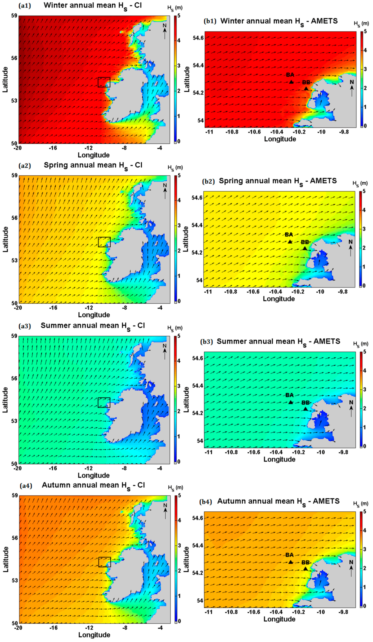
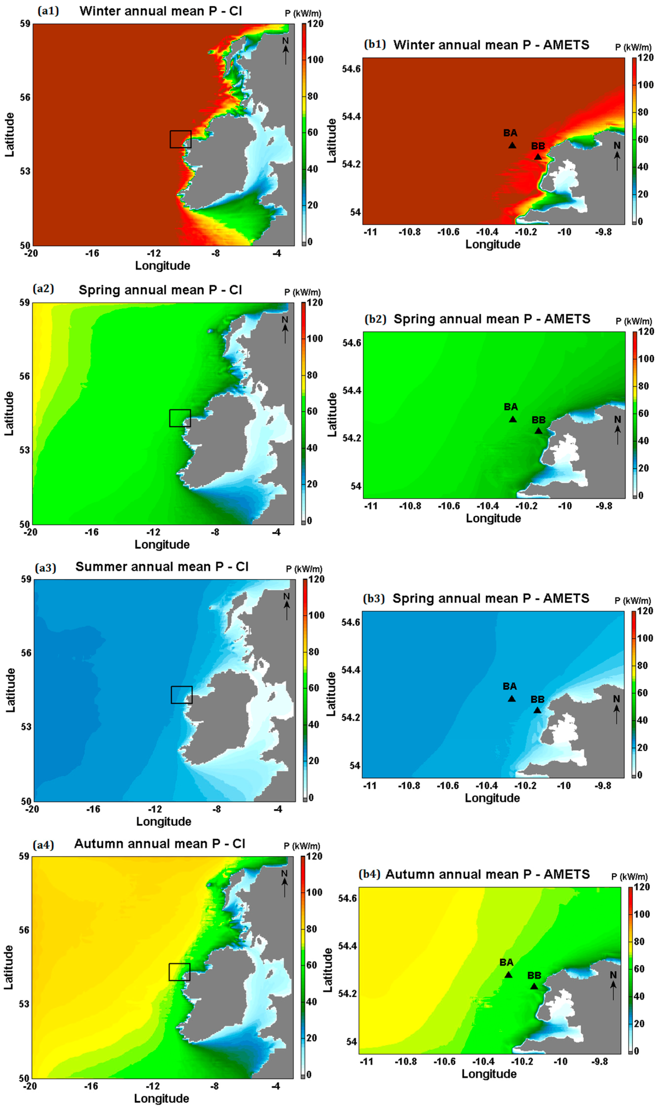
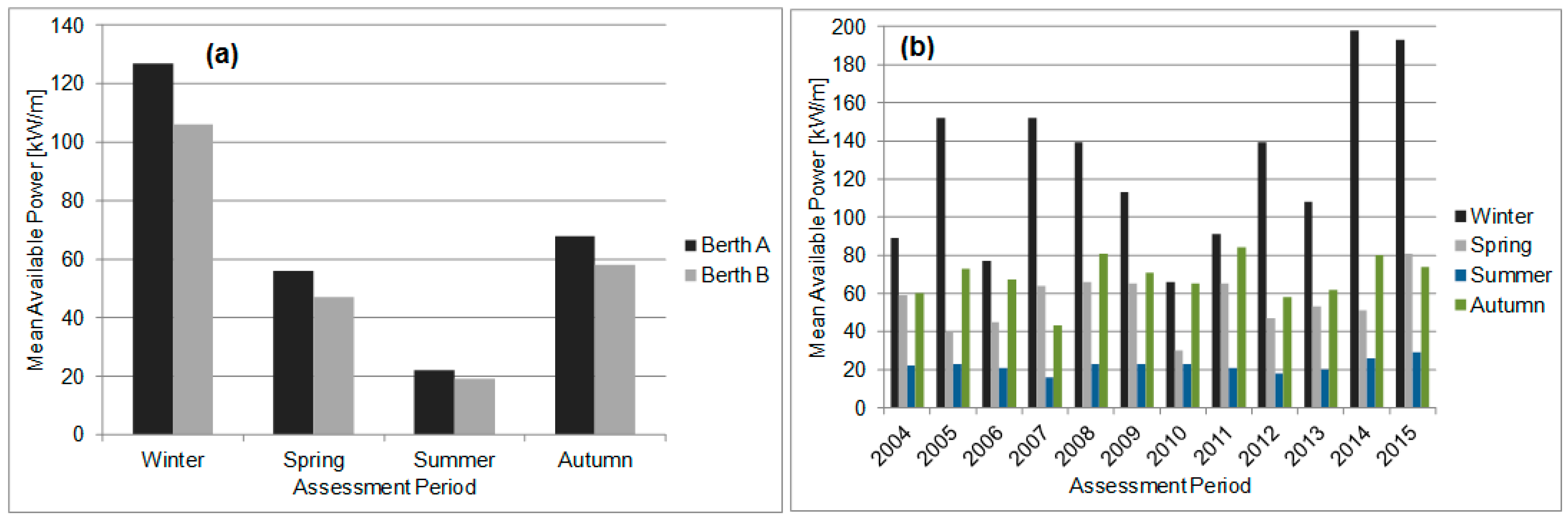
  • There is significant seasonal variation in the wave resource at AMETS—the 12-year mean winter power at BA was 127 kW/m compared to 22 kW/m in summer while mean autumn and spring powers were approximately 60 kW/m. AMETS thus provides a wide range of conditions for testing devices from relatively benign summer sea states to the highly energetic winter sea states; this may provide a useful test strategy where devices are first deployed in summer, then spring/autumn and finally winter. It is also important for device developers to take account of this seasonal variability when designing wave devices for the highly energetic waters off the west coast of Ireland.
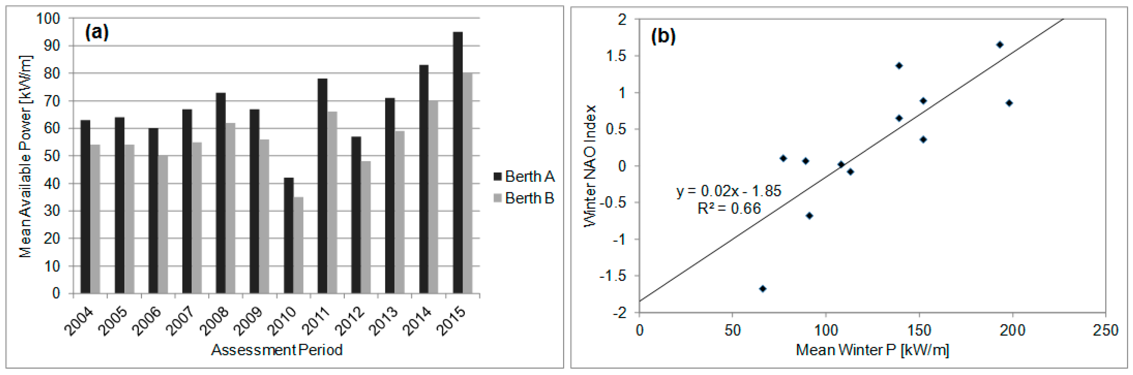
  • There is significant annual variability in wave resource at AMETS. Given that conditions at AMETS would be reflective of conditions off the Irish west coast, it is recommended that any wave resource assessment of Irish Atlantic waters should be based on a minimum of 10 years data. The strong correlation was between mean winter wave powers and the winter NAO index means that where there is limited wave data at an Irish Atlantic site, the winter NAO index could be used to indicate whether the resource estimates are likely to be under- over-representative. Given the decadal variation in NAO it would also be interesting to conduct the AMETS resource assessment for a multi-decadal period.
  • The sea states that contribute most energy at AMETS are not the same as those that occur most often; they are of slightly higher Hs and slightly longer TE. It is extremely important that this mismatch in conditions be considered by device developers when aiming to optimise device performance for particular sea states.

Acknowledgments

This material is based upon works supported by Science Foundation Ireland under Grant No. 12/RC/2302 through MaREI, the national centre for Marine and Renewable Energy Ireland. The authors wish to acknowledge the DJEI/DES/SFI/HEA Irish Centre for High-End Computing (ICHEC) for the provision of computational facilities and support. The authors would like to thank Marine Institute for providing wave buoys data for this research. The first author gratefully acknowledges the receipt of the College of Engineering & Informatics Fellowship. The third author would also like to acknowledge the support of Science Foundation Ireland through the Career Development Award programme (Grant No. 13/CDA/2200).

Author Contributions

Reduan Atan did the numerical modelling and drafted the manuscript. Jamie Goggins and Stephen Nash supervised the research and edited the manuscript. All authors read and approved the manuscript.

Conflicts of Interest

The authors declare no conflict of interest.

Appendix A

Table A1. Summary statistics from annual and seasonal analyses of Hs (m) at BA.
YearAnnualWinterSpringSummerAutumn
MeanSDMaxMeanSDMaxMeanSDMaxMeanSDMaxMeanSDMax
20043.21.610.03.91.57.73.21.58.52.20.95.53.31.38.3
20053.11.713.84.62.113.82.81.17.42.20.95.83.51.69.3
20063.11.610.13.61.48.92.91.28.12.11.06.93.31.69.6
20073.01.710.94.81.810.92.91.69.11.80.75.72.71.06.7
20083.31.711.64.51.910.23.11.811.62.20.85.43.61.610.5
20093.21.610.64.11.710.63.31.48.12.11.15.83.41.510.4
20102.71.311.53.41.48.92.41.07.02.20.96.23.31.511.5
20113.51.612.83.61.712.83.41.29.32.10.96.53.91.38.5
20123.11.510.04.71.611.82.81.49.22.10.85.23.31.17.3
20133.21.710.84.11.710.43.11.38.22.10.96.23.21.59.4
20143.61.712.05.61.710.83.01.26.82.30.95.43.71.39.6
20153.72.012.45.22.112.43.61.69.52.41.07.03.31.88.9
2004–20153.21.613.84.41.913.83.01.411.62.10.97.03.41.511.5
Table A2. Summary statistics from annual and seasonal analyses of Hs (m) at BB.
YearAnnualWinterSpringSummerAutumn
MeanSDMaxMeanSDMaxMeanSDMaxMeanSDMaxMeanSDMax
20043.01.49.43.51.37.12.91.47.72.00.95.33.01.27.8
20052.91.513.24.32.013.22.51.07.02.10.85.43.21.58.4
20062.81.59.13.31.38.12.61.17.42.00.96.53.01.58.7
20072.81.510.04.41.610.02.71.48.61.70.75.22.50.96.1
20083.11.610.74.11.89.42.81.710.72.10.85.03.41.59.6
20093.01.59.83.81.69.73.01.37.62.01.05.23.21.49.8
20102.51.110.63.01.27.92.30.96.32.10.85.63.01.410.6
20113.21.510.93.31.510.83.11.28.42.00.86.13.61.28.1
20122.91.39.24.41.510.92.61.38.91.90.74.73.11.06.4
20133.01.69.93.71.69.92.81.27.62.00.85.72.91.48.5
20143.31.611.55.11.69.92.81.16.12.20.84.93.41.28.8
20153.41.811.54.92.011.53.31.58.52.30.96.53.11.68.2
2004–20153.01.413.24.01.713.22.81.310.72.00.86.53.11.410.6
Table A3. Annual and seasonal operational (Op) and extreme (Ext) Hs thresholds (m) at BA.
YearAnnualWinterSpringSummerAutumn
OpExOpExOpExOpExOpEx
20045.57.55.97.45.27.33.55.25.07.5
20055.38.47.310.84.26.13.45.15.88.2
20065.28.35.68.14.45.83.25.65.58.3
20075.58.47.110.05.38.42.74.24.15.6
20085.88.77.29.35.78.13.44.65.98.1
20095.48.26.89.65.47.23.75.35.38.6
20104.37.05.27.63.76.33.45.15.28.0
20115.78.25.87.94.97.13.35.05.97.5
20125.07.86.99.74.57.53.34.44.86.1
20135.49.16.19.84.66.63.24.45.27.4
20145.79.28.110.24.86.33.55.15.48.4
20156.59.28.411.75.88.33.75.96.07.8
2004–20155.58.56.99.84.97.43.45.15.37.9
Table A4. Annual and seasonal Op and Ext Hs thresholds (m) at BB.
YearAnnualWinterSpringSummerAutumn
OpExOpExOpExOpExOpEx
20045.16.95.46.84.96.73.24.94.76.9
20054.97.96.810.24.05.73.24.75.37.7
20064.87.75.17.44.25.43.05.45.17.8
20074.97.76.49.04.87.62.53.93.85.3
20085.48.06.68.55.47.43.14.25.57.6
20095.07.56.38.95.06.73.54.84.97.9
20104.06.34.76.93.45.63.14.74.87.4
20115.27.55.37.24.56.73.14.85.46.9
20124.67.36.49.04.27.23.04.34.45.6
20135.08.35.69.34.26.23.04.24.86.8
20145.28.67.49.44.45.73.34.65.07.8
20156.08.57.710.95.47.63.45.45.47.3
2004–20155.07.86.39.14.66.83.14.74.97.3
Table A5. Summary statistics from annual and seasonal analyses of TE (s) at BA.
YearYearlyWinterSpringSummerAutumn
Mean±SDMaxMean±SDMaxMean±SDMaxMean±SDMaxMean±SDMax
20048.91.914.410.01.613.48.81.713.77.41.311.69.01.713.6
20058.81.917.210.42.417.28.61.613.17.71.311.49.01.713.6
20068.72.015.49.42.115.48.71.712.87.51.412.48.82.014.0
20079.62.015.810.91.815.69.91.815.28.01.313.49.51.414.6
20089.12.015.010.72.015.88.72.015.07.71.311.89.51.713.8
20098.92.115.710.42.115.79.21.914.77.21.410.89.21.714.7
20108.61.715.69.52.014.78.31.411.87.71.411.89.11.715.6
20119.52.015.910.32.215.99.71.714.87.71.311.79.51.614.0
20128.81.915.810.51.615.48.52.015.87.31.211.39.31.613.3
20139.02.215.310.21.815.38.62.113.37.71.411.48.92.014.3
20149.42.115.711.31.715.39.01.915.77.71.411.29.71.714.9
20159.62.216.311.31.916.39.91.815.07.91.413.99.22.114.5
2004–20159.11.917.210.42.017.29.01.915.87.61.413.99.21.815.6
Table A6. Summary statistics from annual and seasonal analyses of TE (s) at BB.
YearYearlyWinterSpringSummerAutumn
Mean±SDMaxMean±SDMaxMean±SDMaxMean±SDMaxMean±SDMax
20048.71.914.59.81.513.38.61.713.67.31.311.58.91.713.5
20058.71.917.410.32.417.48.51.512.97.71.311.28.81.713.6
20068.62.015.39.32.115.38.51.712.77.41.412.38.72.014.1
20079.62.015.810.71.815.69.91.815.37.91.313.49.51.414.7
20089.02.015.110.72.015.88.62.015.17.61.311.89.41.713.9
20098.82.115.510.32.215.59.11.914.77.11.410.69.11.714.6
20108.51.715.69.32.014.68.21.411.57.61.311.69.01.715.6
20119.42.016.310.22.316.39.61.714.87.61.311.89.31.613.7
20128.71.916.110.41.615.38.42.016.17.21.211.39.21.613.2
20138.82.215.510.11.915.58.42.213.37.61.411.38.82.014.2
20149.32.115.711.11.815.18.91.915.77.61.411.29.61.815.2
20159.42.216.411.22.016.49.81.815.07.81.413.99.12.114.6
2004–20158.91.917.410.32.117.48.91.916.17.51.413.99.11.815.6
Table A7. Annual and seasonal Op and Ext TE thresholds (s) at BA.
YearAnnualWinterSpringSummerAutumn
OpExOpExOpExOpExOpEx
200411.513.211.912.811.012.79.111.011.212.6
200511.413.913.315.810.912.69.510.411.313.2
200611.513.912.214.710.912.59.211.911.713.2
200712.214.613.115.112.414.59.512.111.212.7
200811.813.713.015.311.713.69.411.311.713.3
200911.714.513.115.311.514.49.010.211.513.8
201010.912.912.013.910.111.49.511.611.413.9
201111.914.713.215.311.914.39.510.511.413.5
201211.313.412.414.611.014.58.910.611.413.0
201312.014.312.514.911.613.19.510.811.713.4
201412.314.213.414.811.514.09.511.012.014.1
201512.614.513.716.012.413.89.812.012.013.9
2004–201511.814.113.015.011.513.79.411.211.613.3
Table A8. Annual and seasonal Op and Ext TE thresholds (s) at BB.
YearAnnualWinterSpringSummerAutumn
OpExOpExOpExOpExOpEx
200411.413.111.712.410.812.59.010.811.212.6
200511.213.913.315.910.712.79.310.211.313.2
200611.313.812.114.610.812.49.011.811.713.2
200712.114.613.015.112.514.59.412.011.212.7
200811.713.712.915.411.613.59.211.211.713.3
200911.514.413.115.211.414.48.910.011.513.8
201010.712.811.913.710.011.09.311.411.413.9
201111.814.713.215.311.814.39.410.411.413.5
201211.213.412.414.510.814.78.810.611.413.0
201311.814.312.215.011.513.09.410.611.713.4
201412.214.313.314.811.613.99.410.912.014.1
201512.514.513.716.012.213.99.511.712.013.9
2004–201511.714.113.015.011.413.79.211.011.613.3
Table A9. Summary statistics from annual and seasonal analyses of P (kW/m) at BA.
YearAnnualWinterSpringSummerAutumn
MeanSDMaxMeanSDMaxMeanSDMaxMeanSDMaxMeanSDMax
200463756798976363596842922251646061427
20056410615991521771599404132723241637387515
200660826737783563454538121292676783570
20076794841152132841649159416202104338319
200873969271391306746610092723211368186607
20096790769113121769657140423281737192765
201042578886665500303426423252126590888
2011789199391103951655950321242078468446
20125772651139125993477365118171105845272
201371101811108126811535440520211736275612
2014831051077198147846515035426261598077668
20159512712111931931211818956429322447488505
2004–2015689415991271361599566992722252676877888
Table A10. Summary statistics from annual and seasonal analyses of P (kW/m) at BB.
YearAnnualWinterSpringSummerAutumn
MeanSDMaxMeanSDMaxMeanSDMaxMeanSDMaxMeanSDMax
200454636067361293505635419221485252376
2005549314801321581480343629320201386173418
200650695486468465383830519252415670478
20075577705123109705547753214171783733265
20086281780114109572558478020171127073501
2009567665794103657556134420231345977641
201035477535251385252720420211745475753
201166768457481681555140119211837057403
2012486161711710584540666171614875038211
2013598673289110732434531818181455364504
201470901019163122717434129022211316765565
20158010810451671701045687449025261966274429
2004–2015578014801061161480475878019212415865753
Table A11. Annual and seasonal Op and Ext P thresholds (kW/m) at BA.
YearAnnualWinterSpringSummerAutumn
OpExOpExOpExOpExOpEx
200415934619933514332550151127341
20051474583208908821751121174424
20061444541794379720043166159435
20071754843066321714803210687200
200818945431360119040547103193405
200915745329165216034559137143516
2010902821483396320450126139448
201118740821740812431245117181332
20121293862796091054054382116218
20131655472246881142504297149355
201417455541065211525155138148483
2015250565448102319842762173200384
2004–201516546229065812734649129150389
Table A12. Annual and seasonal Op and Ext P thresholds (kW/m) at BB.
YearAnnualWinterSpringSummerAutumn
OpExOpExOpExOpExOpEx
200413428915826914332540127110277
20051223942878108821745101146375
20061213831483659720038149136385
2007142400247536171480288875175
20081593862635131904054186167351
200913037324055216034550111118433
2010742221122666320442100114378
201115734017332912431238106151271
2012109331236517105405357297188
20131394601836171142503778129300
201414547133755111525147112124411
201520750337588619842751143164328
2004–201513739024155712734642108127335

References

  1. Coe, R.G.; Neary, V.S. Review of Methods for Modeling Wave Energy Converter Survival. In Proceedings of the 2nd Marine Energy Technology Symposium (METS), Seattle, WA, USA, 15–18 April 2014.
  2. Folley, M.; Babarit, A.; Child, B.; Forehand, D.; Boyle, L.O.; Silverthorne, K.; Spinneken, J.; Stratigaki, V.; Troch, P. A Review of Numerical Modelling of Wave Energy Converter Arrays. In Proceedings of the 31st International Conference on Ocean, Offshore and Arctic Engineering (OMAE), Rio de Janeiro, Brazil, 1–6 July 2012; pp. 535–545.
  3. Barstow, S.; Mørk, G.; Lønseth, L.; Mathisen, J.P. WorldWaves wave energy resource assessments from the deep ocean to the coast. In Proceedings of the 8th European Wave and Tidal Energy Conference, Uppsala, Sweden, 7–10 September 2009; pp. 149–159.
  4. National Oceanic and Atmospheric Administration (NOAA). National Weather Service: Environmental Modelling Center—NOAA WaveWatch III, NE Atlantic (Global). Available online: http://polar.ncep.noaa.gov/waves/viewer.shtml?-multi_1-NE_atlantic- (accessed on 23 April 2014).
  5. O’Brien, L.; Dudley, J.M.; Dias, F. Extreme wave events in Ireland: 14 680 BP-2012. Nat. Hazards Earth Syst. Sci. 2013, 13, 625–648. [Google Scholar] [CrossRef]
  6. López, I.; Andreu, J.; Ceballos, S.; Martínez de Alegría, I.; Kortabarria, I. Review of wave energy technologies and the necessary power-equipment. Renew. Sustain. Energy Rev. 2013, 27, 413–434. [Google Scholar] [CrossRef]
  7. Fugro. World Wide Wave Statistics (WWWS). Available online: http://www.oceanor.com/Services/WWWS (accessed on 21 April 2014).
  8. Met Éireann. Met Eireann Weather News: Another Record Wave Height Set Today South of Cork. Available online: http://www.met.ie/news/display.asp?ID=243 (accessed on 15 December 2014).
  9. WestWave. WestWave: Converting Ireland’s Wave Energy Potential. Available online: http://www.westwave.ie/location/ (accessed on 28 November 2013).
  10. Met Éireann. The Irish Meteorological Service Online: Display and Download Historical Data. Available online: http://www.met.ie/climate-request/ (accessed on 27 January 2015).
  11. Gulev, S.K.; Grigorieva, V. Variability of the winter wind waves and swell in the North Atlantic and North Pacific as revealed by the voluntary observing ship data. J. Clim. 2006, 19, 5667–5685. [Google Scholar] [CrossRef]
  12. Cahill, B. Characteristics of the Wave Energy Resource at the Atlantic Marine Energy Test Site. Ph.D. Thesis, University College Cork, Cork, Ireland, 2013. [Google Scholar]
  13. The Wamdi Group. The WAM model—A third generation ocean wave prediction model. J. Phys. Oceanogr. 1988, 18, 1775–1810. [Google Scholar]
  14. Tolman, H. Technical Note: User Manual and System Documentation of WAVEWATCH III; Version 4.18; U.S. Department of Commerce: College Park, MD, USA, 2014.
  15. DHI. Wave Modelling in Oceans and Coastal Areas. Available online: http://www.mikebydhi.com/products/mike-21/waves (accessed on 3 July 2014).
  16. Booij, N.; Ris, R.C.; Holthuijsen, L.H. A third-generation wave model for coastal regions: 1. Model description and validation. J. Geophys. Res. Ocean. 1999, 104, 7649–7666. [Google Scholar] [CrossRef]
  17. Rusu, E. Strategies in using numerical waves model in ocean/coastal applications. J. Mar. Sci. Technol. 2011, 19, 58–75. [Google Scholar]
  18. TUDelft. Hydraulic Engineering: SWAN. Available online: http://www.swan.tudelft.nl/ (accessed on 2 February 2014).
  19. Holthuijsen, L.H. Waves in Oceanic and Coastal Waters; Cambridge University Press: New York, NY, USA, 2009; pp. 24–52. [Google Scholar]
  20. Zijlema, M. Computation of wind-wave spectra in coastal waters with SWAN on unstructured grids. Coast. Eng. 2010, 57, 267–277. [Google Scholar] [CrossRef]
  21. Wolf, J.; Hargreaves, J.C.; Flather, R.A. Application of the SWAN Shallow Water Wave Model to Some U.K Coastal Sites; Proudman Oceanographic Laboratory Report No. 57; Proudman Oceanographic Laboratory (POL): Prenton, UK, 2000. [Google Scholar]
  22. Gleizon, P.; Campuzano, F.J.; García, P.C.; Gomez, B.; Martinez, A. Wave energy mapping along the European Atlantic coast. In Proceedings of the 11th European Wave and Tidal Energy Conference (EWTEC), Nante, France, 6–11 September 2015.
  23. Rusu, L.; Guedes Soares, C. Impact of assimilating altimeter data on wave predictions in the western Iberian coast. Ocean Model. 2015, 96, 126–135. [Google Scholar] [CrossRef]
  24. Iglesias, G.; Carballo, R. Wave energy potential along the Death Coast (Spain). Energy 2009, 34, 1963–1975. [Google Scholar] [CrossRef]
  25. Marine Institute. Online Wave Forecasts. Available online: http://www.marine.ie/Home/site-area/data-services/marine-forecasts/wave-forecasts (accessed on 24 February 2015).
  26. Atan, R.; Goggins, J.; Nash, S. A preliminary assessment of the wave characteristics at the Atlantic Marine Energy Test Site (AMETS) using SWAN. In Proceedings of the 11th European Wave and Tidal Energy Conference (EWTEC), Nantes, France, 6–11 September 2015.
  27. Dee, D.P.; Uppala, S.M.; Simmons, A.J.; Berrisford, P.; Poli, P.; Kobayashi, S.; Andrae, U.; Balmaseda, M.A.; Balsamo, G.; Bauer, P.; et al. The ERA-Interim reanalysis: Configuration and performance of the data assimilation system. Q. J. R. Meteorol. Soc. 2011, 137, 553–597. [Google Scholar] [CrossRef]
  28. U.S. Navy Fleet Numerical Meteorology and Oceanography Center (FNMOC)’s Wave Watch 3 (WW3). Available online: http://gcmd.nasa.gov/records/GCMD_FNMOC_WaveWatchIII.html (accessed on 2 October 2014).
  29. Amante, C.; Eakins, B. ETOPO1 1 Arc-Minute Global Relief Model: Procedures, Data Sources and Analysis. Available online: http://www.ngdc.noaa.gov/mgg/global/global.html (accessed on 8 May 2014).
  30. National Research Council Canada (NRC). Blue KenueTM: Software Tool for Hydraulic Modellers. Available online: http://www.nrc-cnrc.gc.ca/eng/solutions/advisory/blue_kenue_index.html (accessed on 4 February 2014).
  31. Komen, G.J.; Hasselmann, S.; Hasselmann, K. On the existence of a fully developed wind-sea spectrum. J. Phys. Oceanogr. 1984, 14, 1271–1285. [Google Scholar] [CrossRef]
  32. Yan, L. An Improved Wind Input Source Term for Third Generation Ocean Wave Modelling (Wetenschapplijke Rapport); WR-No 87-8; Koninklijk Nederlands Meteorologisch Inistituut: De Bilt, The Netherlands, 1987. [Google Scholar]
  33. Janssen, P.A.E.M. Quasi-linear theory of wind-wave generation applied to wave forecasting. J. Phys. Oceanogr. 1991, 21, 1631–1642. [Google Scholar] [CrossRef]
  34. TUDelft. SWAN Scientific and Technical Documentation—Cycle III Version 41.01A. Available online: http://swanmodel.sourceforge.net/online_doc/swantech/swantech.html (accessed on 25 January 2014).
  35. Hasselmann, K. On the spectral dissipation of ocean waves due to whitecapping. Bound.-Layer Meteorl. 1974, 6, 107–127. [Google Scholar]
  36. Atan, R.; Goggins, J.; Nash, S. Development of a Nested Local Scale Wave Model for a 1/4 Scale Wave Energy Test Site using SWAN. J. Oper. Oceanogr. 2016. submitted. [Google Scholar]
  37. Marine Institute. Wave Buoy Network Real Time Data 30 Minute. Available online: http://data.marine.ie/Dataset/Details/20969# (accessed on 20 January 2015).
  38. Kuik, A.J.; Van Vledder, G.P.; Holthuijsen, L.H. A method for the routine analysis of pitch-and-roll buoy wave data. J. Phys. Oceanogr. 1988, 18, 1020–1034. [Google Scholar] [CrossRef]
  39. Krogstad, H.E.; Trulsen, K. Interpretations and observations of ocean wave spectra. Ocean Dyn. 2010, 60, 973–991. [Google Scholar] [CrossRef]
  40. Gallagher, S.; Gleeson, E.; Tiron, R.; McGrath, R.; Dias, F. Wave climate projections for Ireland for the end of the 21st century including analysis of EC-Earth winds over the North Atlantic Ocean. Int. J. Climatol. 2016, 36, 4592–4609. [Google Scholar] [CrossRef]
  41. Guide to Wave Analysis and Forecasting, 2nd ed.; World Meteorological Organization (WMO): Geneva, Switzerland, 1998.
  42. Data and Products—Data Processing and Interpretation. Available online: http://www.infomar.ie/data/DataProcessing.php (accessed on 5 October 2014).
  43. Atan, R.; Goggins, J.; Nash, S. Development of a high resolution wave model at AMETS using SWAN. In Proceedings of the Civil Engineering Research in Ireland (CERI) Conference, Galway, Ireland, 29–30 August 2016.
  44. Bento, A.R.; Martinho, P.; Campos, R.; Guedes Soares, C. Modelling Wave Energy Resources in the Irish West Coast. In Proceedings of the ASME 2011 30th International Conference on Ocean, Offshore and Arctic Engineering, Rotterdam, The Netherlands, 19–24 June 2011; pp. 945–953.
  45. Demirbilek, Z.; Vincent, C.L. Coastal Engineering Manual, Part II, Water Wave Mechanics, 2nd ed.; Engineer Manual 1110-2-1100; U.S. Army Corps of Engineers: Washington, DC, USA, Chapter 1.
  46. Cornett, A.M. A global wave energy resource assessment. In Proceedings of the Eighteen International Offshore and Polar Engineering Conference, Vancouver, BC, Canada, 6–11 July 2008; International Society of Offshore and Polar Engineers (ISOPE): Cupertino, CA, USA, 2008; pp. 1–9. [Google Scholar]
  47. Atan, R.; Goggins, J.; Harnett, M.; Agostinho, P.; Nash, S. Assessment of wave characteristics and resource variability at a 1/4-scale wave energy test site in Galway Bay using Waverider and high frequency radar (CODAR) data. Ocean Eng. 2016, 117, 272–291. [Google Scholar] [CrossRef]
  48. Drew, B.; Plummer, A.R.; Sahinkaya, M.N. A review of wave energy converter technology. Proc. Inst. Mech. Eng. A J. Power Energy 2009, 223, 887–902. [Google Scholar] [CrossRef]
  49. Ocean Energy Systems (OES). Offshore Installations Worldwide. Available online: http://www.ocean-energy-systems.org/ocean-energy-in-the-world/gis-map/ (accessed on 24 February 2015).
  50. Cahill, B.G.; Lewis, T. Wave energy resource characterisation of the Atlantic Marine Energy Test Site. Int. J. Mar. Energy 2013, 1, 3–15. [Google Scholar] [CrossRef]
  51. Hurrell, J.W. Decadal trends in the North Atlantic Oscillation: Regional temperatures and precipitation. Science 1995, 269, 676–679. [Google Scholar] [CrossRef] [PubMed]
  52. Tsimplis, A.M.N.; Woolf, D.K.; Osborn, T.J.; Wakelin, S.; Wolf, J.; Flather, R.; Shaw, A.G.; Woodworth, P.; Challenor, P.; Blackman, D.; et al. Towards a vulnerability assessment of the UK and northern European coasts: The role of regional climate variab. Philos. Trans. Math. Phys. Eng. Sci. 2005, 363, 1329–1358. [Google Scholar] [CrossRef] [PubMed]
  53. Neill, S.P.; Lewis, M.J.; Hashemi, M.R.; Slater, E.; Lawrence, J.; Spall, S.A. Inter-annual and inter-seasonal variability of the Orkney wave power resource. Appl. Energy 2014, 132, 339–348. [Google Scholar] [CrossRef]
  54. National Oceanic and Atmospheric Administration (NOAA). National Weather Service: North Atlantic Oscilation (NOA). Available online: http://www.cpc.ncep.noaa.gov/products/precip/CWlink/pna/nao.shtml (accessed on 12 June 2016).
Figure 1. Extents of domains and wave buoy locations for (a) coarse Ireland (CI) and (b) Atlantic Marine Energy Test Site (AMETS) wave models. WH: West Hebrides; BS: Black Stone; and GBTS: Galway Bay test site.
Energies 09 00967 g001
Figure 2. Comparison of modelled and measured data at (a1a3) M4 and (b1b3) M6 for 2013. 1 = Hs, 2 = Tz and 3 = MWD. Note: measured MWD was not available for M6.
Energies 09 00967 g002
Figure 3. Comparison of modelled and measured Hs, Tz and MWD at (a1a3) BA and (b1b3) BB for 2013.
Energies 09 00967 g003
Figure 4. Graphical representation of site characterisation approach using (a) percentage of occurrences and (b) normalised wave parameters with percentiles [47].
Energies 09 00967 g004
Figure 5. 12-year annual means of Hs (m) and MWD for (a) CI model and (b) AMETS model.
Energies 09 00967 g005
Figure 6. 12-year seasonal means of Hs (m) and MWD for (a1a4) CI model and (b1b4) AMETS model.
Energies 09 00967 g006
Figure 7. Summary statistics from annual and seasonal analyses of Hs (m) for mean and maximum (Max) at (a) BA and (b) BB.
Energies 09 00967 g007
Figure 8. Annual and seasonal operational (Op) and extreme (Ext) Hs thresholds (m) at (a) BA and (b) BB.
Energies 09 00967 g008
Figure 9. 12-year wave roses between Hs and MWD at (a) BA and (b) BB.
Energies 09 00967 g009
Figure 10. 12-year seasonal wave roses between Hs and MWD at (a1a4) BA and (b1b4) BB.
Energies 09 00967 g010
Figure 11. 12-year annual means of TE (s) and MWD for (a) CI model and (b) AMETS model.
Energies 09 00967 g011
Figure 12. 12-year seasonal mean of TE (s) and MWD for (a1a4) CI model and (b1b4) AMETS model.
Energies 09 00967 g012
Figure 13. Summary statistics from annual and seasonal analyses of TE (s) for mean and maximum (Max) at (a) BA and (b) BB.
Energies 09 00967 g013
Figure 14. Annual and seasonal operational (Op) and extreme (Ext) TE thresholds (s) at (a) BA and (b) BB.
Energies 09 00967 g014
Figure 15. 12-year wave roses between TE and MWD at (a) BA and (b) BB.
Energies 09 00967 g015
Figure 16. 12-year seasonal wave roses between TE and MWD at (a1a4) BA and (b1b4) BB.
Energies 09 00967 g016
Figure 17. 12-year annual means of P (kW/m) for (a) CI model and (b) AMETS model.
Energies 09 00967 g017
Figure 18. 12-year seasonal means of P (kW/m) for (a1a4) CI model and (b1b4) AMETS model.
Energies 09 00967 g018
Figure 19. Summary statistics from annual and seasonal analyses of P (kW/m) for mean and maximum (Max) at (a1,a2) BA and (b1,b2) BB.
Energies 09 00967 g019
Figure 20. Annual and seasonal operational (Op) and extreme (Ext) P thresholds (kW/m) at (a) BA and (b) BB.
Energies 09 00967 g020
Figure 21. Bi-variate scatter plot for (a) BA and (b) BB for 2004–2015 showing percentage occurrences of Hs and TE, with wave power isolines included.
Energies 09 00967 g021
Figure 22. Bi-variate scatter plot for BA for (a) winter; (b) spring; (c) summer; and (d) autumn showing percentage of occurrences of Hs and TE, with wave power isolines included.
Energies 09 00967 g022
Figure 23. Bi-variate scatter plot for BB for (a) winter (b) spring (c) summer and (d) autumn showing percentage of occurrences of Hs and TE, with wave power isolines included.
Energies 09 00967 g023
Figure 24. (a) Seasonal mean powers at BA and BB and (b) inter-annual comparison of seasonal mean P at BA.
Energies 09 00967 g024
Figure 25. (a) Annual mean P at BA and BB and (b) regression analysis of winter North Atlantic Oscillation (NAO) index against winter mean wave power at BA.
Energies 09 00967 g025
Figure 26. 12-year seasonal variability index (SV) values for (a) CI and (b) AMETS model domains.
Energies 09 00967 g026
Figure 27. 12-year monthly variability index (MV) values for (a) CI and (b) AMETS model domains.
Energies 09 00967 g027
Figure 28. Bi-variate scatter plots for (a) BA and (b) BB for 2004–2015 showing numbers of occurrence (in hours) and contribution to total energy of Hs and TE, with wave power isolines included.
Energies 09 00967 g028
Table 1. Summary of available measured wave data. BA: Berth A; BB: Berth B; WH: West-hebrides; and BS: Blackstones.
StationLocationsDepth (m)AvailabilityMeasured Data ResolutionModelled Data Resolution
BA10.3 W, 54.28 N100January 2012 to date30 min30 min
BB10.15 W, 54.23 N50January 2010 to date30 min30 min
M310.55 W, 51.22 N155January 2007 to date1 h1 h
M49.99 W, 54.99 N80January 2008 to date1 h1 h
M615.88 W, 53.07 N3280January 2007 to date1 h1 h
WH7.91 W, 57.29 N83January 2009 to date1 h1 h
BS7.06 W, 56.06 N93January 2009 to date1 h1 h
Table 2. Summary of coarse Ireland (CI) model validation values and measured mean values for 2008–2013. NA indicates non-available data. MWD: mean wave direction.
StationWavesMeanR2RMSEBiasSI
BAHs (m)3.01 m0.950.55 m−0.02 m0.18
Tz (s)6.82 s0.841.22 s0.23 s0.18
MWD (°)285°0.6128°−12°0.10
BBHs (m)2.80 m0.920.69 m−0.40 m0.24
Tz (s)6.98 s0.771.74 s0.23 s0.25
MWD (°)292°0.5725°−4°0.09
M3Hs (m)2.99 m0.950.51 m0.11 m0.17
Tz (s)6.91 s0.851.16 s0.37 s0.17
MWD (°)266°0.7927°0.10
M4Hs (m)3.09m0.920.65 m0.07 m0.21
Tz (s)6.97s0.841.16 s0.27 s0.17
MWD (°)260°0.6160°0.20
M6Hs (m)3.09 m0.920.67 m0.33 m0.22
Tz (s)7.26 s0.841.06 s0.39 s0.15
MWD (°)NANANA°NANA
WHHs (m)2.84 m0.900.85 m0.01 m0.30
Tz (s)6.64 s0.801.47 s0.13 s0.22
MWD (°)265°0.4082°−15°0.30
BSHs (m)2.49 m0.930.60 m0.31 m0.24
Tz (s)1.54 s0.861.42 s0.51 s0.23
MWD (°)268°0.6254°−4°0.20
Table 3. Summary of AMETS model validation values and measured mean values at BA (2012–2013) and BB (2010–2013). NA indicates non-available data.
StationWavesMeanR2RMSEBiasSI
BAHs (m)3.01 m0.950.58 m0.10 m0.19
Tz (s)6.82 s0.871.21 s0.19 s0.18
MWD (°)285°0.6627°−8°0.09
BBHs (m)2.80 m0.950.52 m0.17 m0.22
Tz (s)6.98 s0.801.40 s0.01 s0.20
MWD (°)292°0.6426°−9°0.09
[44] at BBHs (m)2.08 m0.890.48 m0.17 m0.23
Tz (s)8.47 s0.771.42 s1.12 s0.17
MWD (°)NANANA°NANA
[12] at BBHs (m)NA0.840.73 m−0.11 m0.31
Tz (s)NA0.521.82 s−1.15 s0.21
MWD (°)NANANA°NANA
[40] at BBHs (m)2.87 m0.950.41 m0.19 m0.14
Tz (s)7.06 s0.890.86 s0.65 s0.12
MWD (°)NANANA°NANA
Table 4. Summary of deep water waves condition at BA and BB.
Period/LocationDepth, d (m)Mean Wavelength, λ (m)d/λ > 1/2
12-year BA10089.01.1
12-year BB5081.70.6
12-year Winter BB50106.30.5
12-year Spring BB5079.80.6
12-year Summer BB5057.40.9
12-year Autumn BB5083.70.6

