A Long-Term Wind Speed Ensemble Forecasting System with Weather Adapted Correction

Abstract

Wind forecasting is critical in the wind power industry, yet forecasting errors often exist. In order to effectively correct the forecasting error, this study develops a weather adapted bias correction scheme on the basis of an average bias-correction method, which considers the deviation of estimated biases associated with the difference in weather type within each unit of the statistical sample. This method is tested by an ensemble forecasting system based on the Weather Research and Forecasting (WRF) model. This system provides high resolution wind speed deterministic forecasts using 40 members generated by initial perturbations and multi-physical schemes. The forecasting system outputs 28–52 h predictions with a temporal resolution of 15 min, and is evaluated against collocated anemometer towers observations at six wind fields located on the east coast of China. Results show that the information contained in weather types produces an improvement in the forecast bias correction.

1. Introduction

As a kind of clean energy, wind power is receiving increasing attention and application in the world, under the recent concern about energy crisis and global warming issues [1,2]. However, a wind field’s output power strongly depends on local real-time wind speed and is thus uncontrollable. The fluctuation of wind speed will inevitably lead to the fluctuation of the output power of the wind farm. As a result, in order to stabilize the voltage in the power grid, the portion of wind power in the regional power grid must be limited to a certain level, namely the wind power penetration limit [3]. This penetration limit severely restricts wind power’s extensive application.

One solution to this problem is to provide near surface wind speed forecasts with a high temporal resolution, from which the predictions of wind fields’ output power can be obtained [4]. This method has been proven effective in numerous practices [5]. However, because of imperfect models and uncertain initial conditions, errors always exist in numerical weather prediction (NWP) output [6]. In this case, a statistical correction to NWP is an effective means to reduce prediction errors without the potentially expensive cost to improve the model scheme and initial fields [7,8,9,10]. There has been a lot of work testing and improving various statistical correction methods in order to improve the forecast skill of NWPs [1]. Typical approaches include comparison and combination of different statistical models [11,12,13,14] and NWP datasets [15], and incorporating more input parameters.

Generally speaking, statistical correction is to construct a statistical model between historical prediction errors and single or multiple input parameters, in order to estimate the forecast error at the time to be corrected according to the values of these parameters. However, using a single parameter, for example, the predicted value is insufficient in limiting the range of bias estimation. Therefore, improvements have been made by adding more parameters for better estimation accuracy. Previously, parameters to be added in statistical models mostly focus on day/night flag [16], the forecast length [17] and seasonality, as these parameters are physically related to prediction errors and are able to gain along with the prediction. On the other hand, predictions of other meteorological variables besides the wind speed are often added in models. In some works, researchers have proven that the combination of wind direction and wind speed is effective in reducing the error of prediction [18,19], temperature and pressure can also improve the performance of statistical models [20,21], and the spatial interdependency of different variables has been proven to be effective by some studies [22]. However, in many circumstances, especially under complicated weather conditions, these parameters still cannot offer enough information for bias estimation and sometimes even worsen the forecast results, which implies that some additional or more relevant parameters are needed to provide more complete information.

As a summary of the entire regional meteorological field at a certain moment [23], weather type is clearly related to the meteorological conditions and thus the wind field. This parameter not only contains information of seasons, and day and night, but it also reflects environmental conditions in both the local site and the nearby area. In this way, statistical correction models can be equipped with more spatial information compared to those using merely local meteorological factors. While weather classification has been widely used in many fields, such as climate analysis [24,25,26], wind reconstruction [27] and weather prediction [28,29], it has not been conventionally applied or considered in the wind energy field for the forecast bias correction.

In this paper, we define a variable named weather type based on the classification of the meteorological field, and test its effect in improving the long-term wind forecasting skill in a business forecasting system. Compared to traditional bias correction methods, this modified scheme considers typical biases of NWP in different weather types, thus the prediction biases of sampling units can be corrected to an expected value in the same weather type as the focus period. We will show that the addition of weather types has a positive effect in the long-term wind forecasting, and it performs better in ensemble average predictions than non-ensemble predictions due to the higher association between prediction biases and weather types.

The paper is organized as follows. Section 2 describes the weather classification system. Section 3 describes the ensemble forecasting system. Section 4 presents the principle of the correction method. Section 5 shows results and the evaluation. Conclusions and some discussions are given in Section 6.

2. Weather Classification System

2.1. Weather Classification

Weather classification is a methodology that identifies several characteristic weather types by analyzing specific meteorological variables, and then classifies the meteorology fields into these weather types.

In the theory of classification, various cases are divided into several groups, or named clusters. Members in the same group share similar features, while different groups have dissimilar ones [30]. Each group has a “core” showing the representative feature of members in this group. In the case of weather classification, these cores are called characteristic weather types. A characteristic weather type represents the typical distribution of meteorological elements among all of the members in its group. In this way, weather fields are classified into different groups with distinct individual features.

As the background fields of local weather propagate, the weather type at larger scales is usually correlated with local weather processes [23]. Therefore, weather classification can be used for the identification and prediction of various weather processes, and to help improve weather forecast skills.

There are two main approaches to realize weather classification, namely classification of air mass and classification of circulation [30]. The air mass classification refers to the classification typically based on surface variables such as pressure and temperature, which can reflect local weather conditions. On the other hand, circulation classification depends on large-scale parameters such as sea level pressure (SLP), geopotential height, or some other fields that can describe the atmospheric circulation on a regular NWP grid. Compared to air mass classification, the performance of circulation classification is generally superior in that it considers the influence of both large-scale circulation and local meteorological variables [31]. In order to run a circulation classification method, it is necessary to define a domain in advance, so that the algorithm will deal with the distribution of the variables only within this domain, which is also called the “weather case” in this paper.

2.2. Cost733 System

In this research, the European Cooperation in Science and Technology Action 733 (COST733) system [32] is applied to weather classification in China. The COST733 system is originally used to achieve a general numerical method for assessing, comparing and classifying weather situations in Europe, and has demonstrated good performance in previous research [33,34,35]. This system has also been applied to weather classification in areas outside Europe [33], because it has high operability and credibility, and contains plenty of classification schemes.

The clustering algorithm used in this research is the t-mode principal component analysis using oblique rotation [36]. This method can avoid the “snowball effect” to a certain extent, which means most of the sample units are classified as one same type in calculation, and few sample units in other types [37]. This algorithm thus ensures that each type has a relatively comprehensive sample size. The algorithm has already been realized in COST733 [32] (methods: PCT), and has been applied in some published works [38].

2.3. The Operational Process

The operational process is divided into two steps. The first one is to build up characteristic weather types according to historical data, and the second step classifies the cases used in the statistical correction model. A circulation classification system is applied in this research. In this case, a meteorological element called SLP is chosen as the variable considered in the algorithm. Therefore, the word “weather type” in this paper means the distribution of SLP in the selected domain as shown in Figure 1.

Since the characteristic weather types produced by the first step will be used as the classification standard in the next step, it will be beneficial for weather types to be sufficiently representative and stable. These weather types are desired to represent a sufficient number of cases, which naturally requires a large enough historical sample dataset. Therefore, instead of using our NWP outputs, the National Centers for Environmental Prediction (NCEP) Final (FNL) Operational Global Analysis data from 2005 to 2012 is applied which contains ample weather cases in the prediction domain.

Considering that the aims of weather classification is to distinguish the difference between NWP errors of different weather types, enough weather types should be created so that important samples will not be ignored. On the other hand, the number of types should be limited to ensure that all the types have enough samples to keep their representativeness. By testing different numbers of clusters, an 18-weather type model well satisfies the above requirements and is thus applied. Figure 1 shows the circulation patterns of these 18 types.

For example, Types 02 and 03 are two of the most frequently occurring weather types in East China in Figure 1. Type 02 mostly occurs in winter, and it is obvious to see a cold high pressure air mass (red area) over the mainland. In contrast, Type 03 occurs in summer, where the land area is heated and covered by low pressure air masses (blue area), and the West Pacific Ocean is controlled by the well-known subtropical high pressure. The model predictions also have distinguishable performances for these two weather types. For example, the average prediction error of the first type is 2.26 m/s, whereas in another one it is 1.19 m/s.

Once the weather types are established, they will not change in the operational process. When weather cases in either the training set or correction set are input into the statistical model, each of them will be classified and assigned to one of these 18 weather types.

3. The Ensemble Forecasting System

This study is based on the Weather Research and Forecasting (WRF) model [39], which is widely used in research and practical applications. As a meso-scale meteorological model, the WRF model is able to predict weather processes with a resolution of kilometers, and simulates sub-scale processes by parameterization. Vertically, the WRF model uses eta levels to describe pressure layers depending on local surface pressure.

3.1. Ensemble Forecasting

In practice, various uncertainties exist in numerical predictions, including inevitable errors of weather elements in initial prediction fields, differences between physical schemes used and real cases, and defects in forecasting models. In a chaotic systems, such as the atmosphere, any initial uncertainties would lead to a complete loss of forecasting skill. Thus, it is necessary to express the random properties of the atmosphere caused by these uncertainties in predictions [6].

Different from traditional single forecasting, ensemble forecasting makes prediction by using a group of ensemble members to obtain multiple predictions. The idea of ensemble forecasting proposes that by estimating uncertainties of initial values, it will be possible to simulate these errors through the addition of a group of random perturbations to initial values. In this way, we obtain a group of distinct initial values, and each of them will be separately used to run a prediction. Finally, we will get a group of prediction results containing various possibilities in the real case.

There have been several methods to get a single prediction result from ensemble predictions. In this paper, ensemble members are produced by the addition of random perturbations. Therefore, these members should be equal, i.e., it will be unfair to assume any one of the members performing better than the others. In this case, we use the ensemble mean prediction as the final deterministic prediction, which is calculated as the mean value of predictions from all of the ensemble members at the same grid point and the same time.

3.2. Ensemble Member Production

The forecasting system uses the NCEP Global Forecasting System (GFS) data as the initial field. In subsequent processes, by adding random perturbation into the initial field and using multi-physical schemes, an ensemble containing 40 members is produced.

The multi-scheme is a prediction skill that uses different physical parameters and schemes for different members in the ensemble forecasting. In this research, we chose different schemes from four physical processes, which produce 40 different combinations. The multi-scheme includes three microphysics (MP) process schemes (Lin scheme [40], WRF single moment (WSM) three-class simple ice scheme [41], WSM six-class scheme [42]), four land surface (SFC) schemes (thermal diffusion scheme (from Mesoscale Model 5), unified Noah land-surface model [43], the Rapid Update Cycle (RUC) land-surface model [44], and Pleim-Xu scheme [45]), three cumulus (CU) schemes (Kain–Fritsch [46], Betts–Miller [47], and Grell–Devenyi [48]), and two planet boundary layer (PBL) schemes (the Yonsei University [49], and the Mellor–Yamada–Janjić [50]). The

Table A1. Number of ensemble members and schemes used in multi-scheme system.

Microphysics	Surface	Cumulus	Boundary Layer
14 Lin	4 thermal diffusion scheme	2 Kain–Fritsch	1 YSU; 1 MYJ
		1 Betts–Miller	1 YSU
		1 Grell–Devenyi	1 YSU
	4 unified Noah	2 Kain–Fritsch	1 YSU; 1 MYJ
		1 Betts–Miller	1 YSU
		1 Grell–Devenyi	1 YSU
	3 RUC	1 Kain–Fritsch	1 YSU
		1 Betts–Miller
		1 Grell–Devenyi
	3 Pleim-Xu	1 Kain–Fritsch	1 YSU
		1 Betts–Miller
		1 Grell–Devenyi
13 WSM 3-class simple ice scheme	3 thermal diffusion scheme	1 Kain–Fritsch	1 YSU
		1 Betts–Miller
		1 Grell–Devenyi
	4 unified Noah	2 Kain–Fritsch	1 YSU; 1 MYJ 1 YSU 1 YSU
		1 Betts–Miller
		1 Grell–Devenyi
	3 RUC	1 Kain–Fritsch	YSU
		1 Betts–Miller
		1 Grell–Devenyi
	3 Pleim-Xu	1 Kain–Fritsch	YSU
		1 Betts–Miller
		1 Grell–Devenyi
13 WSM 6-class scheme	3 thermal diffusion scheme	1 Kain–Fritsch	YSU
		1 Betts–Miller
		1 Grell–Devenyi
	4 unified Noah	2 Kain–Fritsch	1 YSU; 1 MYJ 1 YSU 1 YSU
		1 Betts–Miller
		1 Grell–Devenyi
	3 RUC	1 Kain–Fritsch	YSU
		1 Betts–Miller
		1 Grell–Devenyi
	3 Pleim-Xu	1 Kain–Fritsch	YSU
		1 Betts–Miller
		1 Grell–Devenyi

in the appendix lists the combination of physical schemes for each ensemble member.

3.3. Forecasting System Design

The wind farms chosen in this research are located on the east coast of China, which are shown in Figure 2. The local observational data comes from anemometer towers in these wind farms, which is average wind speed with a 15 min temporal resolution, in accordance with the requirements of the State Grid Corporation of China (Beijing, China). The height of the wind tower is 70 m, which is consistent with the hub height of wind turbines.

In Section 2.3, the process of classification has been divided into two steps, namely, creating weather types and classifying some other data into these types. This research uses NCEP FNL Operational Global Analysis data from 2005 to 2012 to obtain 18 characteristic weather types. Then in the second step, the WRF ensemble average forecasts from September 2013 to August 2014 are classified into the 18 weather types obtained from the NCEP data. A statistical association is established between forecast biases and weather types for this period, which is subsequently applied to the correction procedure. Ensemble forecasts from September 2014 to January 2015 are used to test the weather adapted correction method.

According to the requirement of the State Grid Corporation of China, the forecasting system needs to publish the prediction of wind speed of the second day at 8:00 am LST (Local Standard Time, Beijing, UTC + 8). Considering the delay in the publishing and receiving of GFS data, and the time cost of simulation, the forecasting system chooses the 12:00 GMT (Greenwich Mean Time) GFS global field to be the initial field, therefore the output prediction is 28–52 h ahead.

In this research, a single domain is constructed with a horizontal resolution of 13.5 km. This domain in Figure 3 contains 409*341 grid points, covering the entire land area of China. Considering the requirement of near surface predictions, the eta levels in the model are set with an increasing density near surface, with four levels located below 100 m above the ground. The time step in the simulation is set to be 60 s in order to increase the stability of model.

Finally the system output field is the ensemble mean of the 40 members. The 70 m wind speed of target wind farms is extracted by spatial interpolation from the output field to be the NWP primary deterministic product, followed by the statistical correction presented below.

4. Statistical Correction

In numerical simulation, the error of prediction comes from two aspects, namely the error of the initial field and the defects of numerical models. Generally speaking, the model error can be divided into the systematic error and the random error [51]. Comparing with random errors, the systematic error can be estimated and reduced through statistical methods, by comparing with historical data. This method is called the statistical correction to numerical predictions, through which the prediction errors could be reduced, and the forecasting result could be improved. In fact, model defects are unavoidable, thus it is effective and necessary to develop statistical correction methods that are based on historical experience to improve model prediction skill.

The statistical correction methods can be generally divided into two categories [51]. The first is posterior correction, which means to make correction to the final output after the numerical integration of the model; the second is to periodically modify the variables along the model integration. In this research, the posterior correction method is applied in the forecasting system.

In this paper, the statistical correction model includes two parts. In this model, the prediction error is processed in the form of average error in 6 h-periods, which is defined as the bias. Here the word “bias” refers to the average value of errors during one period, according to the conventional usage in the field of wind energy forecasting [52]. Firstly, the model estimates the typical biases of wind predictions in different weather types, according to the historical predictions from September 2013 to August 2014. Then in the next step, real-time prediction biases are estimated, which are finally used to correct the prediction results. Typical biases produced by the first part are applied here to improve the bias estimation. This correction method is tested by the forecasts from September 2014 to January 2015.

4.1. Average Bias Correction

The correction method in this research is based on the average bias correction method, a low-cost, widely used method in wind energy predictions. It uses 15 days before the focus day as the training data, or namely, the statistical sample. The method equally divides each day into four segments with 6 h in each, defined as a “period”, and then calculates the average forecast errors for each period. In each of the four periods of the focus day, the forecasting biases are separately estimated as the average error of the historical periods in the same segment of the sample. For the ith segment, we have:

$$bia{s}_i={\displaystyle \sum _{N=1}^{15}}(fc{t}_{i,N}-rea{l}_{i,N})/15$$

(1)

where $fc{t}_{i,N}$ and the $rea{l}_{i,N}$ are, respectively, the average value of the predictions and the observations of wind speed in the ith period of the previous Nth day. The value $bia{s}_i$ is regarded as the estimation of bias in the ith period of the focus day, and the real-time prediction $fc{t}_i$ in this period will be corrected by the value of $bia{s}_i$.

$$fc{t}_{i,new}=fc{t}_i-bia{s}_i$$

(2)

4.2. Combined Correction Method

In this brief correction method, a group of historical predictions are used to estimate the biases of focus predictions. However, the NWP model may have different prediction biases in each of the 18 weather types. Considering that the historical data usually contains different weather types from the focus period, it would lead to a deviation of the estimation.

Besides the wind speed forecasting, the prediction data also include the SLP fields, which makes it possible to link them with the NCEP SLP data and get them classified into the same clusters. When these predictions get classified according to their SLP fields, their wind speed forecasts are also clustered at the same time. In the assumption of sufficient association between the performance of wind predictions and the SLP weather types, the distribution of wind speed prediction biases will be dissimilar in different weather types. In this case, it will be reasonable to add weather types into the wind bias estimation method to further improve forecasting results.

In this section, we refine the average bias correction by considering the association between prediction biases of sample units and corresponding weather types, and attempt to reduce the bias caused by using units with different weather types to estimate the target forecasting bias.

Firstly, we use the FNL analysis data from 2005 to 2012 to build up the classification model. The FNL data are published four times each day with a six-hour interval. Thus, it is possible to classify the target wind fields in each 6-hour period, and the statistical sample volume is large enough to support a classification of 18 weather types. In the next step, the ensemble average predictions from September 2013 to August 2014 are classified according to the weather types produced by the FNL SLP data. Then, for each weather type, we calculate the bias distribution of the ensemble average predictions. The probability density function (PDF) is applied to display the distributions of biases in different weather types. The PDFs of the data come from the kernel density estimation, and most of them show a clear monomodal property, which will be shown in the next section. The value where the highest frequency occurs, called the peak value, is used as the “typical bias” of model predictions in this weather type.

In the original correction process, the average bias of each sampling unit is used as the final estimation of the target bias in this period, which is shown in Equation (1). In the refined method, this average bias is further corrected according to the difference between the typical bias of the unit’s weather type and the target period’s weather type.

For example, here we define the variable b to be the typical bias, which is determined by the period’s weather type. Thus, the focus period in the ith segment has a typical bias $b_{i,f}$ according to its weather type. Then we choose 15 days before this day of interest as the training data, and collect 15 periods as the statistical sample which belongs to the same (ith) segment as the focus period. The Nth corresponding period in the sample (named the Nth unit) has a typical bias of $b_{i,N}$, and its prediction bias has been known as the difference between $fc{t}_{i,N}$ and $rea{l}_{i,N}$. The updated estimated bias $bia{s}_{i,new}$ has:

$$bia{s}_{i,new}={\displaystyle \sum _{N=1}^{15}}(fc{t}_{i,N}-rea{l}_{i,N}-(b_{i,N}-b_{i,f}))/15$$

(3)

and is then applied in the same way as the $bia{s}_i$ in Equation (2). Here the value of typical biases, namely $b_{i,N}$ and $b_{i,f}$, only depend on their weather types.

In this way, the prediction bias of a sample unit is corrected to be an estimation of the forecasting bias of this unit in the same weather type of the focus period, thus the weather types of both historical units and the target unit are consistent, and the effectiveness of considering weather types in the correction methods will be directly checked through correction results.

5. Results

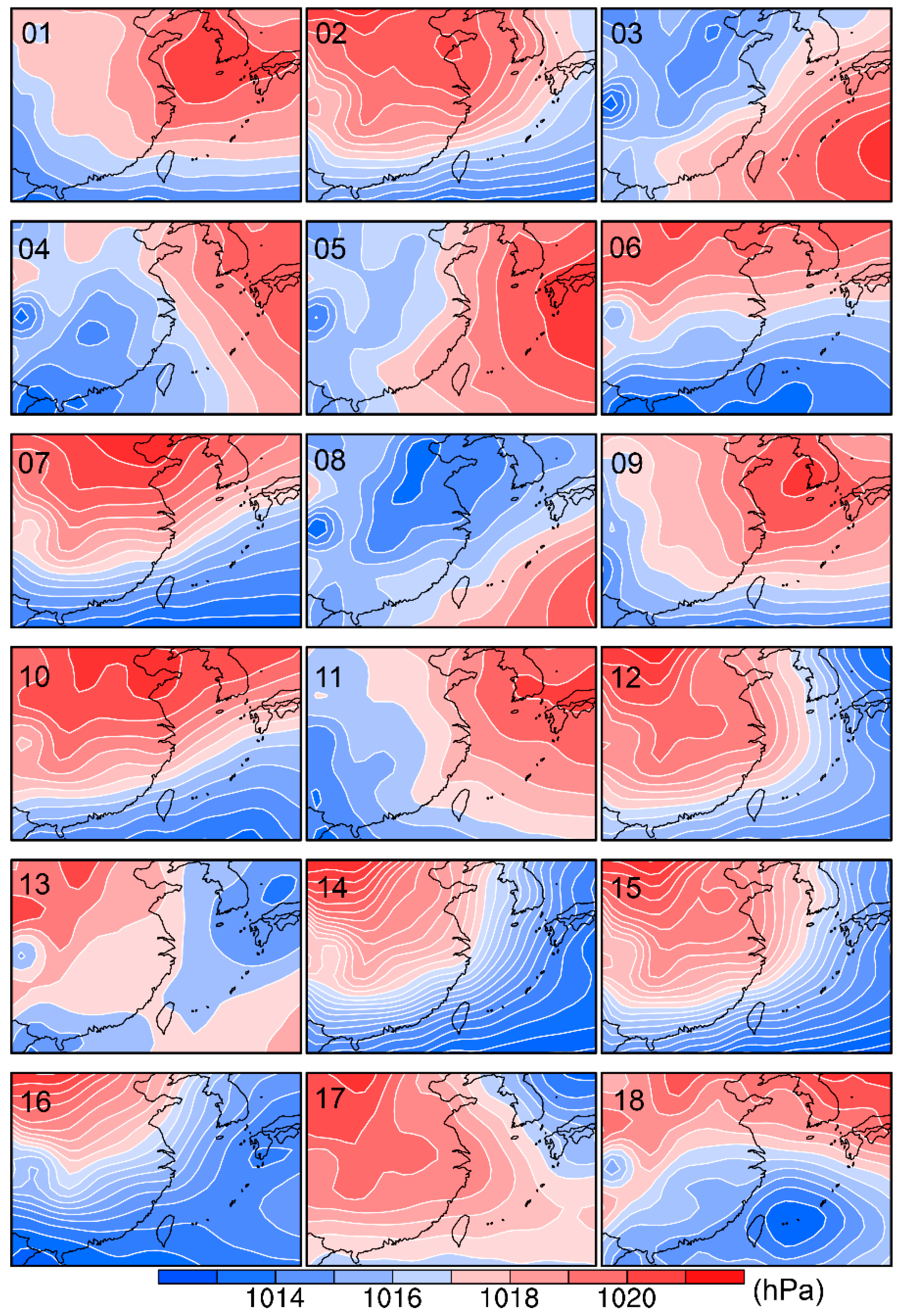
5.1. Weather Classification

In order to evaluate the effect of weather classification, we choose the ensemble average forecasting data of 6 costal wind farms during the period from September 2013 to August 2014. We calculate the DF of prediction biases for each weather type.

Instead of focusing on the specific performances of predictions in each weather type, it is more important to focus on some overall properties in this correction method. Firstly, we check whether most of them follow a monomodal distribution, which serves as an important basis of using the peak values as typical biases. Then, we check if these peak values have obvious differences from the others, which reflects the effectiveness of this correction method.

According to the prediction bias distributions shown in Figure 4, the majority of weather types has a monomodal distribution, although a few have distributions with multiple peaks or no obvious peak. On the other hand, although these curves display an overall common distribution, there are still several discernable groups with different peak values. In other words, the distributions can reflect the impact of weather types on statistical correction, and thus the peak value of the distribution can be set as the typical bias of predictions in the corresponding weather type. The typical biases of six wind fields and 18 weather types have been listed in Appendix A.

Thus far, we have classified all the testing data points into 18 weather type clusters, according to their predicted SLP distributions. For the purpose of bias estimation, we must further evaluate the classification results by analyzing the forecasting biases, which have also been naturally categorized into these clusters. We calculate the average characteristic radius of each weather type cluster and the differentiation degree of the clusters. Here, we define the average characteristic radius $ra{d}_i$, the differentiation degree dis and their ratio K as follows:

$$ra{d}_i=\sqrt{\frac{1}{N}{\displaystyle \sum _{n=1}^N}{(a_{in}-k_i)}^2}$$

(4)

$$dis=\sqrt{\frac{1}{M}{\displaystyle \sum _{i=1}^M}{(k_i-\overline{k_i})}^2}$$

(5)

$$K=dis/ra{d}_i$$

(6)

where for a cluster with the number i, the corresponding cluster element set is $a_{in}$, the value of the cluster center is $k_i$, and M is total number of clusters.

As $ra{d}_i$ reflects the tightness of each cluster and $dis$ indicates the separation among different clusters, the value K can be used as an index of clustering validation. A higher K means higher concentration level of single clusters, and the larger distance between different clusters, in other words the effect of clustering is more significant [53].

A control experiment is set here for the same period as ensemble forecasts, which had a single member without perturbation and multi-scheme treatment. The result listed in

Table 1. Cluster index K of control predictions (K con) and ensemble forecasts (K ens).

Wind Field	K con	K ens
001	0.28	0.45
002	0.20	0.43
003	0.17	0.43
004	0.30	0.45
005	0.29	0.56
006	0.24	0.55
average	0.25	0.48

below shows that the ensemble forecast biases have a more reasonable clustering structure. It means compared to the single forecasts, the ensemble average predictions have a higher association between forecasting biases and weather types in weather classification, because when grouped into the previously defined weather types, the biases among different groups become more distinguishable.

5.2. Ensemble Forecast Evaluation

To evaluate the ensemble forecasting, the sample comes from six wind farms on the east coast of Chin, during September 2014 to January 2015. In this section, we examine the effect of ensemble forecasts with weather adapted correction with 28–52 h lead time.

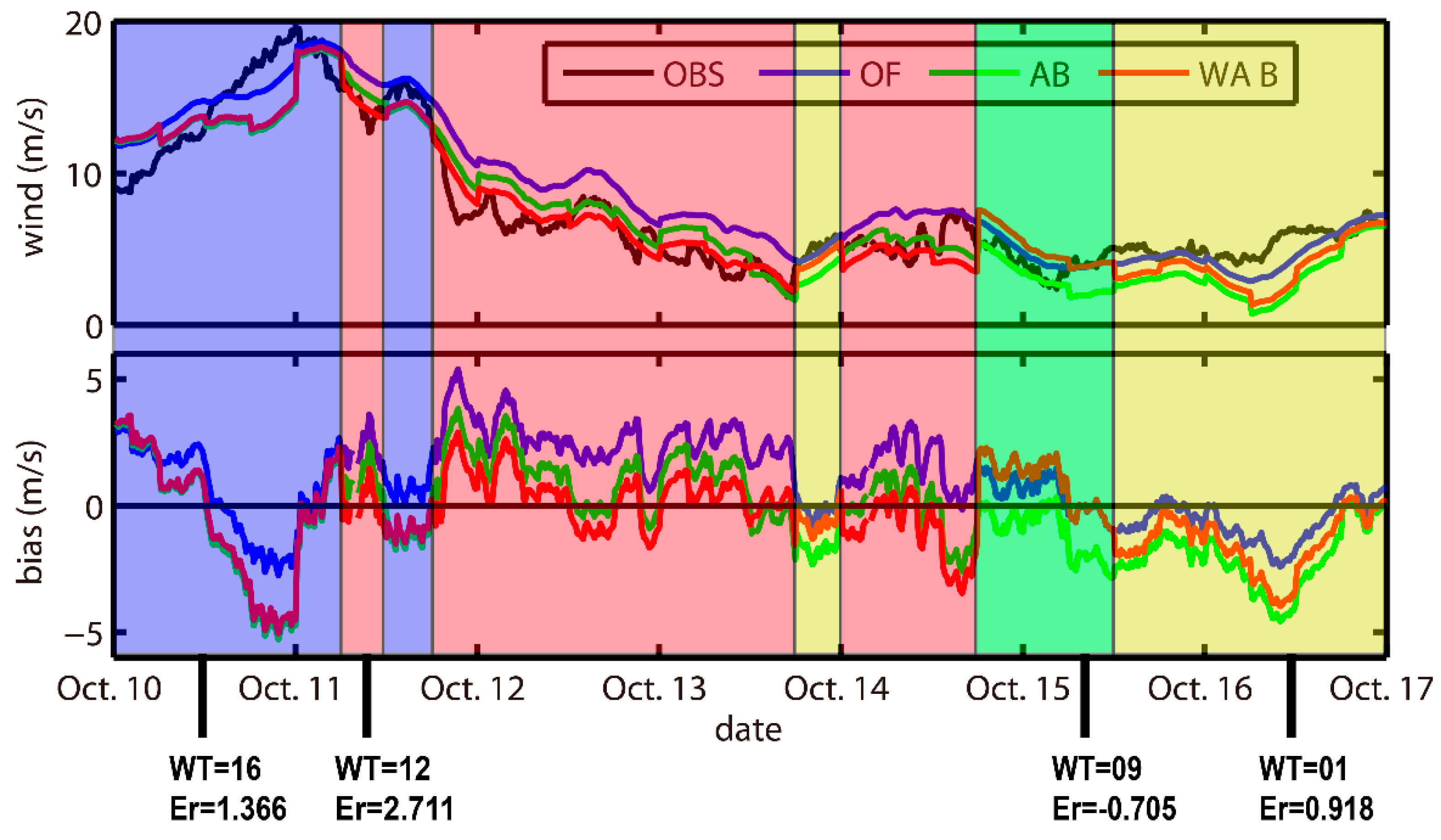
5.2.1. Deterministic Forecasting

When evaluating the deterministic forecasting of specific meteorological variables at a single site, root mean square error (RMSE) is one of the metrics that are commonly used. The variable reflects the overall level of prediction errors in the whole statistical sample. It can be calculated by the prediction error $e_i$, which is the difference between forecast value $v_i$ and observation value $o_i$, with a sample size of N.

$$RMSE=\sqrt{\frac{1}{N}{\displaystyle \sum _i^N}{e_i}^2}$$

(7)

In discussion of ensemble prediction errors, Hou et al. [54] made the following decomposition of RMSE with the reference work by Takacs [55].

$$RMS{E}^2=mnbia{s}^2+sd{e}^2=mnbia{s}^2+sdbia{s}^2+dis{p}^2$$

(8)

where:

$$mnbias=\overline{e_i}$$

(9)

$$sde=\mathsf{\sigma }(e_i)$$

(10)

$$sdbias=\mathsf{\sigma }(v_i)-\mathsf{\sigma }(o_i)$$

(11)

$$disp=\sqrt{2\mathsf{\sigma }(v_i)\ast \mathsf{\sigma }(o_i)\ast (1-r(v_i,o_i))}$$

(12)

$\mathsf{\sigma }(v_i)$ and $\mathsf{\sigma }(o_i)$ are standard deviations of predictions $v_i$ and observations $o_i$, and $r(v_i,o_i)$ is the correlation coefficient between predictions and observations.

In this operation, RMSE is divided into two parts: the mean bias of predictions mnbias and the standard deviation of prediction biases sde. Here, the mnbias reflects a continuous overall deviation of predictions, while the sde indicates the fluctuation of forecast errors around mnbias. Then, sde is further decomposed into two parts: sdbias and disp. sdbias is the difference between the standard deviation of predictions and observations, which refers to the bias of predictions with respect to the degree of wind speed fluctuation. sdbias reflects the systematic error together with mnbias, which could be reduced by posterior statistical correction. Dispersion error disp represents the part of forecast error that is more difficult to be corrected, because this part of error comes from phase shifts instead of amplitude [55].

In this test, control predictions with a single member (SINGLE) are compared with the ensemble average predictions (ENS). The original forecasts (OF) from the two forecasting systems are corrected by either the average bias correction method (AB) or the refined weather type adapted bias correction method (WAB). All these six predictions are evaluated by daily averaged RMSE. The results are listed in

Table 2. Daily average RMSE (m/s) of six predictions, including original forecasts (OF), average bias correction (AB), and weather adapted bias correction (WAB) results of the single member predictions (SINGLE) and the ensemble predictions (ENS).

Wind Field	SINGLE			ENS
	OF	AB	WAB	OF	AB	WAB
001	2.68	2.29	2.21	2.71	2.09	1.86
002	3.41	2.87	2.75	2.83	2.14	1.90
003	3.22	2.80	2.74	2.70	2.09	1.96
004	1.53	1.53	1.63	2.42	1.95	1.84
005	2.94	2.56	2.45	3.01	2.35	2.17
006	2.47	2.29	2.28	2.23	1.95	1.78
average	2.71	2.39	2.34	2.65	2.10	1.92

.

According to the result, RMSE shows that ensemble forecasts keep a higher accuracy in both the original forecasts and the corrected predictions. In addition, the average bias correction performs well in reducing the error of both ensemble forecasts and single forecasts, and the weather adapted correction outperforms the traditional correction. Moreover, the improvement by weather type correction is more significant in ensemble predictions than in single forecasts in the tested wind farms. Results of further analysis on RMSE of ensemble predictions are listed in

Table 3. Mean bias (m/s) and change rate K (%) of original forecasts (OF), average bias correction (AB), and weather adapted bias correction (WAB) outputs from the ensemble average forecasts.

Wind Field	OF	AB	${\mathit{K}}_{\mathit{A}\mathit{B}}$	WAB	${\mathit{K}}_{\mathit{W}\mathit{A}\mathit{B}}$
001	2.40	0.68	0.72	0.64	0.73
002	2.47	0.81	0.67	0.78	0.68
003	2.33	0.77	0.67	0.75	0.68
004	1.95	0.68	0.65	0.62	0.68
005	2.57	0.85	0.67	0.80	0.69
006	1.67	0.51	0.70	0.46	0.72
average	2.23	0.72	0.68	0.68	0.70

,

Table 4. Standard deviation bias (m/s) and change rate K (%) of three outputs of ensemble average forecasts.

Wind Field	OF	AB	${\mathit{K}}_{\mathit{A}\mathit{B}}$	WAB	${\mathit{K}}_{\mathit{W}\mathit{A}\mathit{B}}$
001	0.77	0.89	−0.16	0.65	0.16
002	0.64	0.75	−0.17	0.48	0.25
003	0.46	0.55	−0.18	0.38	0.18
004	0.44	0.52	−0.17	0.42	0.05
005	0.75	0.85	−0.14	0.61	0.18
006	0.50	0.57	−0.14	0.31	0.38
average	0.59	0.69	−0.16	0.47	0.20

and

Table 5. Dispersion error (m/s) and change rate K (%) of three outputs of ensemble forecasts.

Wind Field	OF	AB	${\mathit{K}}_{\mathit{A}\mathit{B}}$	WAB	${\mathit{K}}_{\mathit{W}\mathit{A}\mathit{B}}$
001	2.13	2.34	−0.09	2.15	−0.01
002	2.26	2.43	−0.08	2.24	0.01
003	2.26	2.43	−0.07	2.31	−0.02
004	2.18	2.28	−0.05	2.19	−0.01
005	2.47	2.65	−0.07	2.51	−0.01
006	2.22	2.32	−0.04	2.17	0.02
average	2.25	2.41	−0.07	2.26	−0.00

.

Setting the original ensemble forecasts as the reference forecasts, we further define the ratio of change that is made by two correction methods as follows for quantitative comparison:

$$K_{var}=1-\frac{var}{va{r}_{ref}}$$

(13)

In the above equation, var is the evaluation index of the forecasts to be tested, and $va{r}_{ref}$ is the index of reference forecasts. $K_{var}$ indicates the capability of the correction method in reducing prediction errors. $K_{var}$ is positive only when prediction errors are reduced. The higher $K_{var}$ is, the better the correction method performs.

From these three tables, we can compare two correction methods quantitatively by the K index for the three scenarios. The average bias correction makes a very huge improvement in the mean bias of predictions (Table 3), but it does not help improve sdbias (Table 4) and disp (Table 5), which even have a growth. By incorporating weather classification to the correction, the growth of sdbias caused by correction has been reduced, as highlighted in Table 4, and the disp index also shows improvements. Nonetheless, little influence is seen in mnbias.

5.2.2. Continuous Ranked Probability Skill (CRPS)

The continuous ranked probability skill (CRPS) is widely used in evaluation of ensemble systems. Compared with the mean absolute error (MAE) and RMSE that evaluate the error of a deterministic forecasting, the CRPS considers the performance of all ensemble members. The CRPS reflects the difference of cumulative distribution function (CDF) between the full ensemble forecasts and the observations, and is usually used as an assessment of overall performance of ensemble prediction systems.

For the prediction variable x, an ensemble prediction contains multiple members, and each member outputs prediction values for N times in the period of interest. Therefore, all of these members are time series of prediction values with the length of N. It can always obtain the probability density $\mathsf{\rho }(x)$ of prediction values of all the members at the same snapshot, namely, the ith time point. Then we have the CDF $F_i^f(x)$ as:

$$F_i^f(x)={\displaystyle {\int }_{-\infty }^x}\mathsf{\rho }(y)dy$$

(14)

Therefore the $F_i^f(x)$ is the probability that the member forecast will be smaller than x.

On the other hand, at the same time point we have the observed value $x_i^a$. Thus, we establish the CDF of the corresponding observation $F_i^o(x)$ as:

$$F_i^o(x)=H(x-x_i^a)$$

(15)

where:

$$H(x)=\{\begin{array}{l}0 \text{for} x<0\\ 1 \text{for} x\ge 0\end{array}$$

(16)

is known as the Heaviside function [56,57].

Thus, the $F_i^o(x)$ shows a Boolean value of whether the observed value $x_i^a$ is smaller than x.

Then, the CRPS is computed by the formula:

$$CRPS=\frac{1}{N}{\displaystyle \sum _{i=1}^N{\int }_{-\infty }^{\infty }}{[F_i^f(x)-F_i^o(x)]}^{2}dx$$

(17)

showing the difference between the predicted and observed cumulative distributions.

Here, the CRPS of the original and corrected ensemble forecasts are given in

Table 6. Continuous ranked probability skill (CRPS) of original (OF), AB and WAB corrected ensemble forecasts.

Wind Field	OF	AB	WAB
001	2.10	1.58	1.39
002	2.20	1.62	1.44
003	2.09	1.56	1.45
004	1.52	1.41	1.33
005	2.37	1.80	1.63
006	1.71	1.43	1.30
average	2.00	1.57	1.42

.

The CRPS score (CRPSS) is further used here to compare impacts of two correction methods, which is defined as follows [57]:

$$CRPSS=1-CRPS/CRP{S}_{OF}$$

(18)

The CRPS is the index of corrected predictions, and $CRP{S}_{OF}$ is the original predictions as a reference. For the six wind farms in test, the CRPSS of two correction methods are shown in Figure 5, which shows that WAB forecast is stable and an improvement against AB forecast (CRPSS around 7% increment).

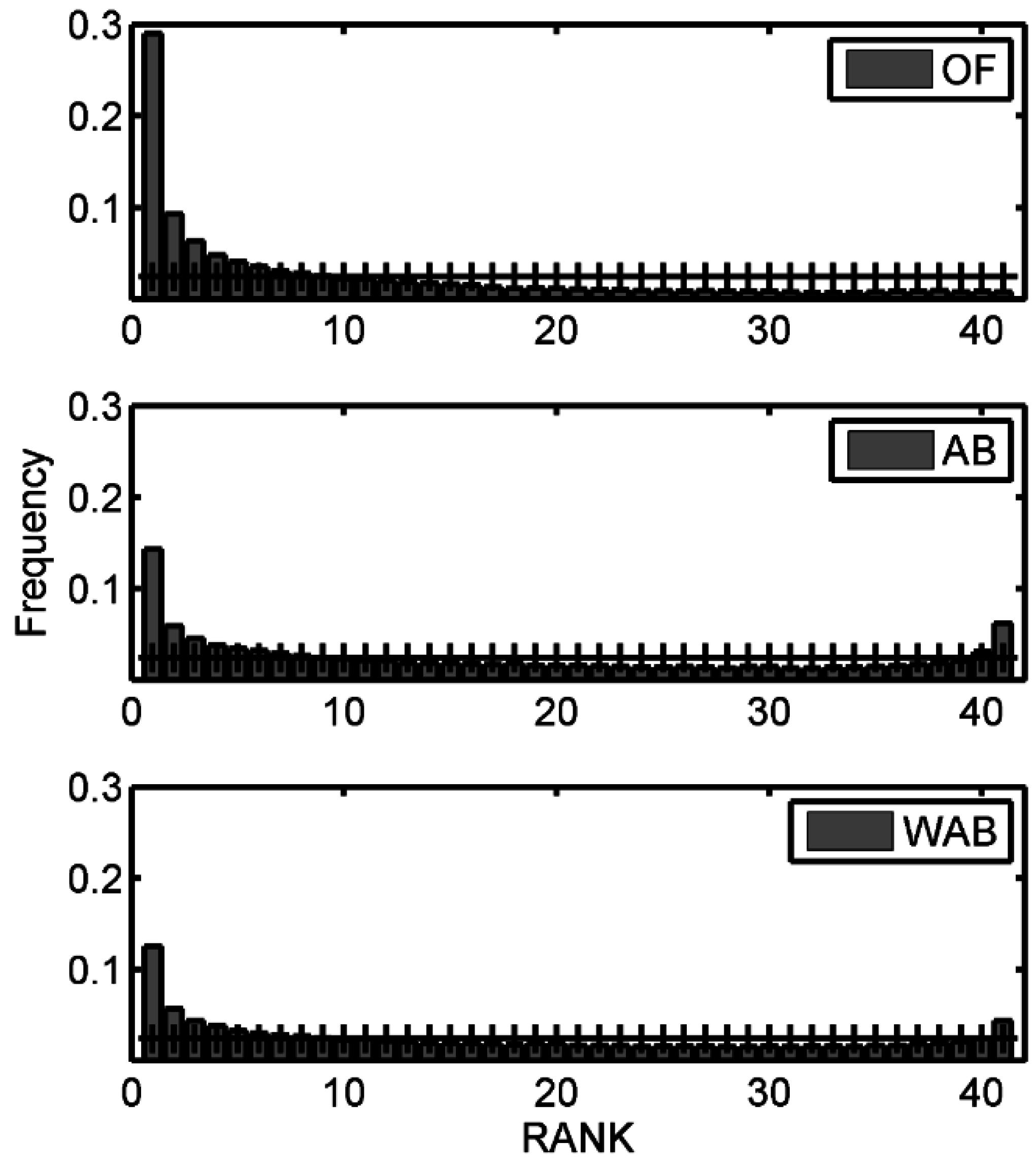
5.2.3. Rank Histogram

As a method to directly reflect the consistency in statistical distributions between ensemble members’ predictions and observation, rank histogram is widely used in evaluation of the reliability of ensemble predictions [58,59]. In this method, at each snap shot, the wind speed is divided into N + 1 intervals by N forecast values of ensemble members, and the frequency that observation values fall in each interval is counted. In the ideal situation, the probability density distribution of ensemble members’ prediction values should be consistent with that of observations, thus the observation should fall in each interval with the same probability, which means the rank histogram will have a flat distribution [58,59] (the black solid line in Figure 6). For the three predictions, data from all wind farms are used as the sample here.

In the upper panel of Figure 6, the rank histogram of original forecast (OF) has an “L” shaped distribution, which means the dominant part of ensemble members have larger prediction values than observation. The middle panel shows that the errors of predictions are effectively reduced after AB correction, producing a “U” shaped rank histogram. Nonetheless, some observations are still beyond the upper boundary of ensemble forecasts after correction, meaning that the predictions have been excessively corrected. The lower panel shows the histogram of predictions with a WAB correction. The excessive correction is mediated, and observations that fall below the lower boundary are further reduced.

6. Conclusions and Discussion

In this research, an ensemble forecast system with 40 members is presented by adding initial random perturbations and multi-schemes to the GFS global forecasting fields. The forecasting system provides deterministic 70 m wind speed predictions of single wind farms with a 15 min interval. These forecasting results are further improved by developing a weather adapted bias correction scheme, based upon the average bias correction method. The effects of correction methods are tested by ensemble forecasts from September 2014 to January 2015. Observations of 70 m wind speed from wind towers are used as the ground truth, with the same temporal resolution as the predictions.

In the evaluation of the weather classification, ensemble predictions outperform single member forecasts. This is because that compared with single member forecasts, ensemble average forecasts come from 40 different members, and have filtered out uncertainty factors of single members. In this way, it tends to achieve a more stable performance under different weather types, and has been proven to be better than single forecasts by various scoring methods [60], thus leading to a higher association between the prediction biases and the weather type.

In the assessment of ensemble predictions, the deterministic predictions and the performances of all ensemble members are tested. The weather adapted correction outperformed conventional correction in both of the above two aspects.

The mean bias of predictions (mnbias) refers to a continuous systematic deviation in predictions, while sdbias reflects the difference between standard deviations of predictions and observation values, and disp comes from phase shifts. It is usually much easier to use historical data to decrease the value of mnbias than sdbias and disp, because mnbias has a strong persistence than others, and could be effectively reduced by a simple subtraction. By contrast, it would be more skillful to correct the intensity of fluctuation and the phase variation.

In the AB correction method, an idealized assumption is that the 6 h averaged bias of predictions changes smoothly over time, while large fluctuations often occur in the practical forecast. These fluctuations will cause a deviation of bias estimation to subsequent predictions, and lead to an inadequate or excess correction. This type of error in the correction is one of the main factors that cause an increase in sdbias.

By considering the impact of different weather types on prediction biases, the WAB correction method proposed in this research estimates and corrects prediction bias fluctuations caused by the development of weather processes, and reduces the inadequate or excess correction caused by sudden severe changes of 6 h average prediction biases. Therefore, compared with the AB correction method, the WAB correction method improves the prediction by reducing the biases in the standard deviation of predictions.

In Figure 7, four of the 18 weather types are observed during the period of seven days with different statistical typical biases, highlighted by different background colors. The 12th (red area, noted by WT = 12 in Figure 7) weather type has a larger positive bias than the 1st (yellow area) type, which results in an overestimation of prediction biases after 15 October through the bias estimation. The weather adapted correction method successfully reduces the excessive correction with respect to predictions (blue line), and the WAB corrected predictions (red line) show an improvement compared with the AB predictions (green line).

In this research, the refined weather adapted bias correction method is based on the assumption that there is a good association between the local near-surface wind speed in wind farms and the weather types of this area. This also forms the basis of estimating the prediction biases through mesoscale weather fields in NWPs. If the local wind speed in the wind farm has a strong local property, and is rarely influenced by background weather field, the effect of correction would nonetheless deteriorate.

The sample wind farms are located in Jiangsu Province, on the east coast of China, which is a flat area without complex terrain. Therefore, the association between weather types and real wind speed is relatively clear. Similar performance of the newly developed correction method can be expected in offshore wind farms, while the effect may not be as satisfactory in mountainous areas.

References

1. Jung, J.; Broadwater, R.P. Current status and future advances for wind speed and power forecasting. Renew. Sustain. Energy Rev. 2014, 31, 762–777. [Google Scholar] [CrossRef]
2. Zhou, W.; Lou, C.; Li, Z.; Lu, L.; Yang, H. Current status of research on optimum sizing of stand-alone hybrid solar-wind power generation systems. Appl. Energy 2010, 87, 380–389. [Google Scholar] [CrossRef]
3. Christensen, J.F. New control strategies for utilizing power system networks more effectively: The state of the art and the future trends based on a synthesis of the work in the cigre study committee 38. Control Eng. Pract. 1998, 6, 1495–1510. [Google Scholar] [CrossRef]
4. Al-Yahyai, S.; Charabi, Y.; Gastli, A. Review of the use of Numerical Weather Prediction (NWP) Models for wind energy assessment. Renew. Sustain. Energy Rev. 2010, 14, 3192–3198. [Google Scholar] [CrossRef]
5. Milligan, M.R.; Miller, A.H.; Chapman, F. Estimating the Economic Value of Wind Forecasting to Utilities. In Proceedings of the Windpower, Washington, DC, USA, 27–30 March 1995.
6. Kalney, E. Atmospheric Modeling, Data Assimilation, and Predictability; Cambridge University Press: Cambridge, UK, 2003. [Google Scholar]
7. Negnevitsky, M.; Johnson, P.; Santoso, S. Short term wind power forecasting using hybrid intelligent systems. In Proceedings of the 2007 IEEE Power Engineering Society General Meeting, Tampa, FL, USA, 24–28 June 2007; p. 4.
8. Giebel, G.; Kariniotakis, G.; Brownsword, R. The state-of-the-art in short term prediction of wind power from a Danish perspective. J. Virol. 2003, 82, 9513–9524. [Google Scholar]
9. Ma, L.; Luan, S.; Jiang, C.; Liu, H.; Zhang, Y. A review on the forecasting of wind speed and generated power. Renew. Sustain. Energy Rev. 2009, 13, 915–920. [Google Scholar]
10. Soman, S.S.; Zareipour, H.; Malik, O.; Mandal, P. A review of wind power and wind speed forecasting methods with different time horizons. In Proceedings of the North American Power Symposium, Arlington, TX, USA, 26–28 September 2010; pp. 1–8.
11. Pinson, P.; Nielsen, H.A.; Madsen, H.; Kariniotakis, G. Skill forecasting from ensemble predictions of wind power. Appl. Energy 2009, 86, 1326–1334. [Google Scholar] [CrossRef] [Green Version]
12. Zhao, E.; Zhao, J.; Liu, L.; Su, Z.; An, N. Hybrid Wind Speed Prediction Based on a Self-Adaptive ARIMAX Model with an Exogenous WRF Simulation. Energies 2016, 9, 7. [Google Scholar] [CrossRef]
13. Bouzgou, H.; Benoudjit, N. Multiple architecture system for wind speed prediction. Appl. Energy 2011, 88, 2463–2471. [Google Scholar] [CrossRef]
14. Sun, W.; Liu, M.; Liang, Y. Wind Speed Forecasting Based on FEEMD and LSSVM Optimized by the Bat Algorithm. Energies 2015, 8, 6585–6607. [Google Scholar] [CrossRef]
15. Alessandrini, S.; Sperati, S.; Pinson, P. A comparison between the ECMWF and COSMO Ensemble Prediction Systems applied to short-term wind power forecasting on real data. Appl. Energy 2013, 107, 271–280. [Google Scholar] [CrossRef]
16. Traiteur, J.J.; Callicutt, D.J.; Smith, M.; Roy, S.B. A Short-Term Ensemble Wind Speed Forecasting System for Wind Power Applications. J. Appl. Meteorol. Clim. 2012, 51, 1763–1774. [Google Scholar] [CrossRef]
17. Cui, B.; Toth, Z.; Zhu, Y.; Hou, D. Bias Correction for Global Ensemble Forecast. Weather Forecast 2012, 27, 396–410. [Google Scholar] [CrossRef]
18. Erdem, E.; Shi, J. ARMA based approaches for forecasting the tuple of wind speed and direction. Appl. Energy 2011, 88, 1405–1414. [Google Scholar] [CrossRef]
19. Gallego, C.; Pinson, P.; Madsen, H.; Costa, A.; Cuerva, A. Influence of local wind speed and direction on wind power dynamics—Application to offshore very short-term forecasting. Appl. Energy 2011, 88, 4087–4096. [Google Scholar] [CrossRef] [Green Version]
20. De Giorgi, M.G.; Ficarella, A.; Tarantino, M. Assessment of the benefits of numerical weather predictions in wind power forecasting based on statistical methods. Energy 2011, 36, 3968–3978. [Google Scholar] [CrossRef]
21. Cadenas, E.; Rivera, W.; Campos-Amezcua, R.; Heard, C. Wind Speed Prediction Using a Univariate ARIMA Model and a Multivariate NARX Model. Energies 2016, 9, 109. [Google Scholar] [CrossRef]
22. Ambach, D.; Croonenbroeck, C. Space-time short- to medium-term wind speed forecasting. Stat. Methods Appl. 2016, 25, 5–20. [Google Scholar] [CrossRef]
23. Barry, R.G.; Perry, A.H. Synoptic Climatology: Methods and Applications; Routledge Kegan & Paul: Methuen, MA, USA, 1973. [Google Scholar]
24. Spinoni, J.; Szalai, S.; Szentimrey, T.; Lakatos, M.; Bihari, Z.; Nagy, A.; Németh, Á.; Kovács, T.; Mihic, D.; Dacic, M.; et al. Climate of the Carpathian Region in the period 1961–2010: Climatologies and trends of 10 variables. Int. J. Climatol. 2015, 35, 1322–1341. [Google Scholar] [CrossRef]
25. Casado, M.J.; Pastor, M.A. Circulation types and winter precipitation in Spain. Int. J. Climatol. 2016, 36, 2727–2742. [Google Scholar] [CrossRef]
26. Burlando, M. The synoptic-scale surface wind climate regimes of the Mediterranean Sea according to the cluster analysis of ERA-40 wind fields. Theor. Appl. Climatol. 2009, 96, 69–83. [Google Scholar] [CrossRef]
27. Saavedra-Moreno, B.; de la Iglesia, A.; Magdalena-Saiz, J.; Carro-Calvo, L.; Durán, L.; Salcedo-Sanz, S. Surface wind speed reconstruction from synoptic pressure fields: Machine learning versus weather regimes classification techniques. Wind Energy 2014, 18, 1531–1544. [Google Scholar] [CrossRef]
28. Ramos, A.M.; Pires, A.C.; Sousa, P.M.; Trigo, R.M. The use of circulation weather types to predict upwelling activity along the western Iberian Peninsula coast. Cont. Shelf Res. 2013, 69, 38–51. [Google Scholar] [CrossRef]
29. Addor, N.; Rohrer, M.; Furrer, R.; Seibert, J. Propagation of biases in climate models from the synoptic to the regional scale: Implications for bias adjustment. J. Geophys. Res. Atmos. 2016, 121, 2075–2089. [Google Scholar] [CrossRef] [Green Version]
30. Huth, R.; Beck, C.; Philipp, A.; Demuzere, M.; Ustrnul, Z.; Cahynova, M.; Kyselý, J.; Tveito, O.E. Classifications of Atmospheric Circulation Patterns Recent Advances and Applications. Ann. N. Y. Acad. Sci. 2008, 1146, 105–152. [Google Scholar] [CrossRef] [PubMed]
31. Zhang, J.P.; Zhu, T.; Zhang, Q.H.; Li, C.C.; Shu, H.L.; Ying, Y.; Dai, Z.P.; Wang, X.; Liu, X.Y.; Liang, A.M.; et al. The impact of circulation patterns on regional transport pathways and air quality over Beijing and its surroundings. Atmos. Chem. Phys. 2012, 12, 5031–5053. [Google Scholar] [CrossRef]
32. Philipp, A.; Bartholy, J.; Beck, C.; Erpicum, M.; Esteban, P.; Fettweis, X.; Huth, R.; James, P.; Jourdain, S.; Kreienkamp, F.; et al. Cost733cat—A database of weather and circulation type classifications. Phys. Chem. Earth 2010, 35, 360–373. [Google Scholar] [CrossRef]
33. Hoy, A.; Sepp, M.; Matschullat, J. Large-scale atmospheric circulation forms and their impact on air temperature in Europe and northern Asia. Theor. Appl. Climatol. 2013, 113, 643–658. [Google Scholar] [CrossRef]
34. Cahynova, M.; Huth, R. Circulation vs. climatic changes over the Czech Republic: A comprehensive study based on the COST733 database of atmospheric circulation classifications. Phys. Chem. Earth 2010, 35, 422–428. [Google Scholar] [CrossRef]
35. Demuzere, M.; Kassomenos, P.; Philipp, A. The COST733 circulation type classification software: An example for surface ozone concentrations in Central Europe. Theor. Appl. Climatol. 2011, 105, 143–166. [Google Scholar] [CrossRef]
36. Huth, R. A circulation classification scheme applicable in GCM studies. Theor. Appl. Climatol. 2000, 67, 1–18. [Google Scholar] [CrossRef]
37. Huth, R. An intercomparison of computer-assisted circulation classification methods. Int. J. Climatol. 1996, 16, 893–922. [Google Scholar] [CrossRef]
38. Toreti, A.; Fioravanti, G.; Perconti, W.; Desiato, F. Annual and seasonal precipitation over Italy from 1961 to 2006. Int. J. Climatol. 2009, 29, 1976–1987. [Google Scholar] [CrossRef]
39. Skamarock, W.C.; Klemp, J.B. A time-split nonhydrostatic atmospheric model for weather research and forecasting applications. J. Comput. Phys. 2008, 227, 3465–3485. [Google Scholar] [CrossRef]
40. Lin, Y.-L.; Farley, R.D.; Orville, H.D. Bulk Parameterization of the Snow Field in a Cloud Model. J. Clim. Appl. Meteorol. 1983, 22, 1065–1092. [Google Scholar] [CrossRef]
41. Hong, S.-Y.; Dudhia, J.; Chen, S.-H. A Revised Approach to Ice Microphysical Processes for the Bulk Parameterization of Clouds and Precipitation. Mon. Weather Rev. 2004, 132, 103–120. [Google Scholar] [CrossRef]
42. Hong, S.-Y.; Lim, J.-O.J. The WRF single-moment 6-class microphysics scheme (WSM6). J. Korean Meteor. Soc. 2006, 42, 129–151. [Google Scholar]
43. Ek, M.B.; Mitchell, K.E.; Lin, Y.; Rogers, E.; Grunmann, P.; Koren, V.; Gayno, G.; Tarpley, J.D. Implementation of Noah land surface model advances in the National Centers for Environmental Prediction operational mesoscale Eta model. J. Geophys. Res. 2003, 108. [Google Scholar] [CrossRef]
44. Benjamin, S.G.; Dévényi, D.; Weygandt, S.S.; Brundage, K.J.; Brown, J.M.; Grell, G.A.; Kim, D.; Schwartz, B.E.; Smirnova, T.G.; Smith, T.L.; et al. An Hourly Assimilation–Forecast Cycle: The RUC. Mon. Weather Rev. 2004, 132, 495–518. [Google Scholar] [CrossRef]
45. Xiu, A.; Pleim, J.E. Development of a Land Surface Model. Part I: Application in a Mesoscale Meteorological Model. J. Appl. Meteorol. 2001, 40, 192–209. [Google Scholar] [CrossRef]
46. Kain, J.S.; Fritsch, J.M. Convective Parameterization for Mesoscale Models: The Kain-Fritsch Scheme. In The Representation of Cumulus Convection in Numerical Models; Emanuel, K.A., Raymond, D.J., Eds.; American Meteorological Society: Boston, MA, USA, 1993. [Google Scholar]
47. Betts, A.K.; Miller, M.J. The Betts-Miller Scheme. In The Representation of Cumulus Convection in Numerical Models; Emanuel, K.A., Raymond, D.J., Eds.; American Meteorological Society: Boston, MA, USA, 1993. [Google Scholar]
48. Grell, G.A.; Dévényi, D. A generalized approach to parameterizing convection combining ensemble and data assimilation techniques. Geophys. Res. Lett. 2002, 29, 38. [Google Scholar] [CrossRef]
49. Hong, S.-Y.; Noh, Y.; Dudhia, J. A New Vertical Diffusion Package with an Explicit Treatment of Entrainment Processes. Mon. Weather Rev. 2006, 134, 2318–2341. [Google Scholar] [CrossRef]
50. Mellor, G.L.; Yamada, T. Development of a turbulence closure model for geophysical fluid problems. Rev. Geophys. 1982, 20, 851–875. [Google Scholar] [CrossRef]
51. Schemm, C.E.; Unger, D.A.; Faller, A.J. Statistical Corrections to Numerical Predictions III. Mon. Weather Rev. 1981, 109, 96–109. [Google Scholar] [CrossRef]
52. Madsen, H.; Pinson, P.; Kariniotakis, G.; Nielsen, H.A.; Nielsen, T.S. Standardizing the Performance Evaluation of ShortTerm Wind Power Prediction Models. Wind Eng. 2005, 29, 475–489. [Google Scholar] [CrossRef] [Green Version]
53. Calinski, T. A Dendrite Method for Cluster Analysis. Biometrics 1968, 24, 207. [Google Scholar]
54. Hou, D.; Kalnay, E.; Droegemeier, K.K. Objective verification of the SAMEX’98 ensemble forecasts. Mon. Weather Rev. 2001, 129, 73–91. [Google Scholar] [CrossRef]
55. Takacs, L.L. A 2-step scheme for the advection equation with minimized dissipation and dispersion errors. Mon. Weather Rev. 1985, 113, 1050–1065. [Google Scholar] [CrossRef]
56. Hersbach, H. Decomposition of the continuous ranked probability score for ensemble prediction systems. Weather Forecast 2000, 15, 559–570. [Google Scholar] [CrossRef]
57. Alessandrini, S.; Delle Monache, L.; Sperati, S.; Nissen, J.N. A novel application of an analog ensemble for short-term wind power forecasting. Renew. Energy 2015, 76, 768–781. [Google Scholar] [CrossRef]
58. Anderson, J.L. A method for producing and evaluating probabilistic forecasts from ensemble model integrations. J. Clim. 1996, 9, 1518–1530. [Google Scholar] [CrossRef]
59. Hamill, T.M. Interpretation of rank histograms for verifying ensemble forecasts. Mon. Weather Rev. 2001, 129, 550–560. [Google Scholar] [CrossRef]
60. Guidelines on Ensemble Prediction Systems and Forecasting; WMO-No. 1091; World Meteorological Organization (WMO): Geneva, Switzerland, 2012.
Figure 1. 18 weather types created by classification.
Energies 09 00894 g001
Figure 2. Location of the six wind farms used in this study, denoted by black dots.
Energies 09 00894 g002
Figure 3. Domain used in predictions.
Energies 09 00894 g003
Figure 4. Prediction bias distributions of 18 weather types at the six wind farms.
Energies 09 00894 g004
Figure 5. Continuous ranked probability skill (CRPS) score in all tested wind farms, with a comparison between average bias correction (AB) and weather adapted bias correction (WAB).
Energies 09 00894 g005
Figure 6. Rank histogram of ensemble forecasts, including original forecast (OF), and predictions from average bias correction (AB) and weather adapted bias correction (WAB). The black line with marks “+” is the ideal flat distribution.
Energies 09 00894 g006
Figure 7. Original (OF, the blue solid line) and two corrected predictions (AB, the green line and WAB, the red line) outputs and observation data (real, the black), and corresponding forecast biases (solid lines in subplot below), with weather types in each period highlighted by background color. In lines below axis, WT shows the number of each period’s weather type, and Er means the corresponding typical bias of that weather type, which have been listed in Table A2 in Appendix A.
Energies 09 00894 g007